Lagrange's method applied to a Slinky

Abstract

The Lagrange method is applied to two dynamic models of a Slinky, one based on point masses and linear springs and a second where the Slinky is represented as a sequence of half hoops connected by torsion springs. For the first time, the use of Lagrange's method applied to a Slinky has produced a multi-body dynamic model that can potentially with minor modification reproduce all the interesting behaviour Slinkies are well known for; descending stairs, pseudo levitation, transmission of longitudinal and transverse waves. In this paper, the models are derived and a limited exploration of the two dynamic models’ behaviour is considered. For unforced oscillation, the point mass model and torsion spring model produce a similar amplitude and frequency. When considering forced oscillations, the point mass model has a very different spectrum of natural frequencies than the torsion spring model. The torsion spring model is considered for different forcing conditions.

Introduction

A Slinky is a soft spring, made from plastic or steel, see Figure 1. It was invented in the 1940s and patented in 1947 by James. ¹ It has many interesting properties that show the interplay between kinetic energy, elastic potential energy, and gravitational potential energy. If you release a Slinky that is in a vertical orientation the bottom part of the Slinky remains stationary until the top half descends to the point where the tension in the springs reduces such that the weight of the spring is more than the spring force.^2,3 The pseudo levitation property is a counterintuitive behaviour but can be explained by an analysis of a model where the Slinky is represented as a sequence of point masses separated by linear springs. Other interesting properties are an initially vertical Slinky that is forced in an angular direction behaves much like a rope. A Slinky can also be used to demonstrate transverse waves and longitudinal waves depending on orientation and forcing conditions. ⁴ A Slinky can also descend stairs, the original behaviour described by Cunningham ⁵ and Wilson. ⁶

Figure 1.

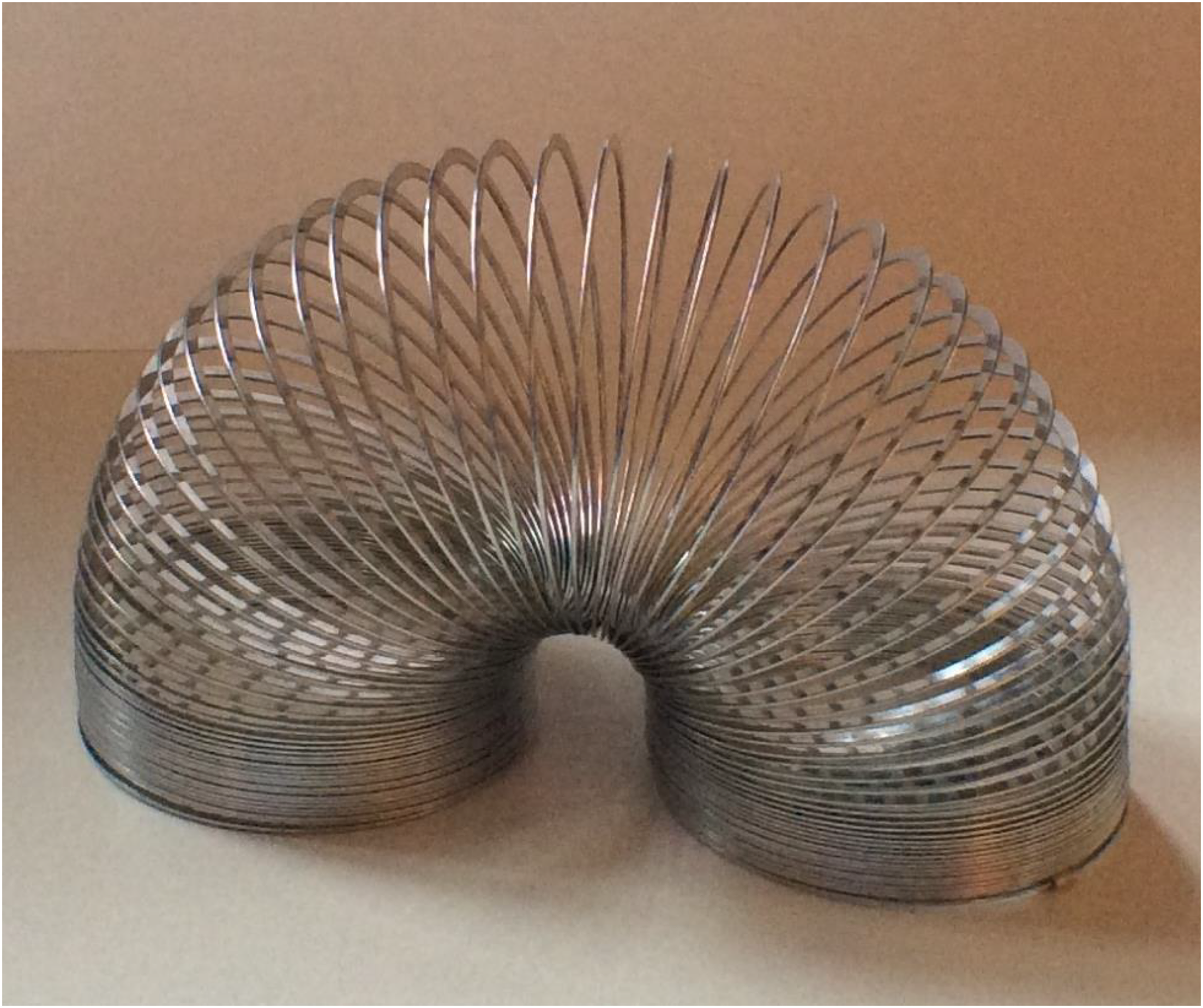
A Slinky in an arch configuration.

A Slinky has long been used in the education of early years undergraduate physicists demonstrating the phenomena discussed above.^7–10 Most educational research has either been of an experimental nature or is based on a mathematical model where the Slinky is represented as a number of point masses separated by linear springs. In the limit of an infinite number of point masses, this model tends towards the wave equation.^11,12 The dynamics of a Slinky is an excellent device for demonstrating principles of mechanics to mechanical engineering students. It is a mechanical system that students are familiar with and are comfortable with.

It is well known that many mechanical engineering students struggle with mechanics, because of its mathematical basis and the weaker students are intimidated by this, or makes the subject matter opaque to them.^13,14 A number of different strategies to address this problem have been investigated. One option is to implement dynamic models, embedded in a virtual learning environment (VLE).^15–18 Equipped with a VLE the student can explore parameter space without initially having a grasp of the mathematical basis of the dynamic model. The argument being the student can grasp the mathematical basis once they have insight into the dynamic behaviour. Another approach to help students gain an understanding of mechanics is to take a familiar model, such as a simple pendulum and demonstrating that such a model has far more complex and interesting behaviour than expected.^19,20

The present article is one of a series that looks to give students insight into dynamic systems they may have experience of, such as a washing machine ²¹ and an unbalanced roller. ²² The papers in the series generally present a model that is derived using material taught in the early years of an undergraduate degree and then extend the model in some way using more advanced concepts. In so doing, students can see the links between the initial courses in mechanics and advanced mechanics courses. In this way, the concept of the ‘jam tomorrow’ argument for why a student should engage with a subject is illustrated in a positive way.

The present article is more advanced than the previous articles in the series as a Slinky is treated as a many body system. The derivation and analysis of many body problems are taught in undergraduate intermediate mechanics courses. This situation is addressed in the paper by initially deriving the point mass representation of a Slinky by applying Newton's second law together with a free body diagram and mass acceleration diagram. A well-understood methodology to first-year mechanical engineering undergraduates. The same system of equations can be derived using Lagrange's method, a more accepted method of derivation for many body dynamical systems.

The paper then goes on to, for the first time, derive a dynamical model of a Slinky represented by a series of half hoops connected by torsional springs. This yields a complicated system of ordinary differential equations (ODEs) that can be solved numerically. The advantage of the torsion spring model of a Slinky is the complex dynamical behaviour of a Slinky described above can be captured. A point mass model of a Slinky can be used to investigate the pseudo levitation property of a Slinky,^2,3 but cannot be used to investigate the other phenomena discussed. The point mass model cannot simulate transverse waves in a Slinky or simulate a Slinky descending a stair. In principle, a torsion spring model could be used to investigate all of these phenomena.

In the literature, there is a model for a Slinky descending a stair, but it is not a many body representation of a Slinky. The Slinky is represented by two bars with a link in the middle. ²³ Holmes et al. ²⁴ presented a model of a Slinky for calculating the equilibrium state of a Slinky for a range of end conditions. Their model included the effects of torsion, shear, and axial stress. More recently, Cumber ²⁵ demonstrated that for many scenarios the torsion spring representation reproduced the behaviour that Holmes et al. ²⁴ investigated. Shear and axial stress are important where the Slinky is on a slope and the slope is slowly increased or the Slinky is attached to two surfaces that are very close to each other relative to the unstretched length of the spring. This is significant as Holmes et al. ²⁴ reported their intention to extend their analysis to produce a dynamic model. At present no dynamic model based on Holmes et al.'s analysis is forthcoming. The representation of a Slinky based on half hoops and torsion springs presented in Cumber ²⁵ is extended here to produce a dynamic model of a Slinky. The ultimate goal is to apply the torsion spring dynamic model to a Slinky descending a stair. For the present article, the motion of a Slinky is restricted to the motion of a Slinky fixed at one end.

Point mass model of a Slinky

In this section, the point mass model is derived using Newton's second law and the Lagrangian approach.

Derivation using Newton's second law

In a point mass model, a Slinky is represented as a sequence of point masses interconnected by linear springs that satisfy Hooke's law. The kinematics of the point mass model is expressed in Figure 2. Applying Newton's second law to a point mass in the middle of the Slinky then from the free body diagram and mass acceleration diagram the differential equation for the jth point mass is

$$m{\ddot{y}}_{C,j}=k_{pt}(y_{C,j-1}-y_{C,j})-k_{pt}(y_{C,j}-y_{C,j+1})+mg$$

(1)

Figure 2.

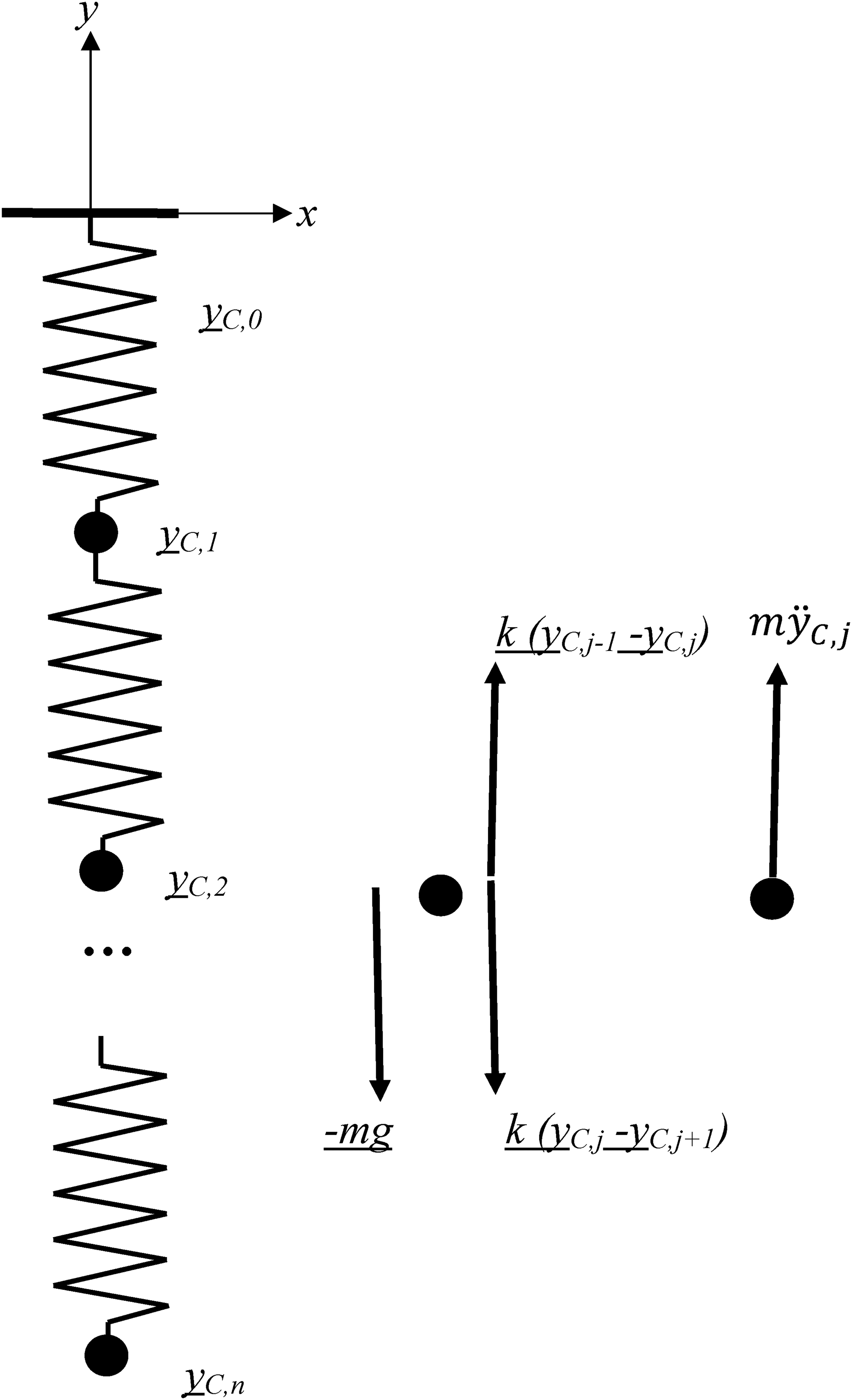
Point mass model of a Slinky, its free body diagram and mass acceleration diagram.

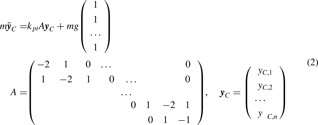
The last point mass, j  =  n, has a slightly different free body diagram, but the derivation is similar. Here k_pt is the linear spring constant. For all point masses, the equations of motion can be represented as

$$\begin{array}{rl}m{\ddot{\mathit{y}}}_C=& k_{pt}A{\mathit{y}}_C+mg\left(\begin{array}{c}\begin{array}{c}1\\ 1\end{array}\\ \begin{array}{c}\dots \\ 1\end{array}\end{array}\right)\\ A=& \left(\begin{array}{ccc}-2& 1& \begin{array}{ccc}0& \dots & \begin{array}{cc}& 0\end{array}\end{array}\\ 1& -2& \begin{array}{ccc}1& 0& \begin{array}{cc}\dots & 0\end{array}\end{array}\\ & & \begin{array}{c}\begin{array}{ccc}\dots & & \end{array}\\ \begin{array}{c}\begin{array}{ccc}\begin{array}{cc}0& 1\end{array}& -2& 1\end{array}\\ \begin{array}{ccc}0& 1& -1\end{array}\end{array}\end{array}\end{array}\right),{\mathit{y}}_C=\left(\begin{array}{c}\begin{array}{c}{y}_{C,1}\\ y_{C,2}\end{array}\\ {\begin{array}{c}\dots \\ y\end{array}}_{C,n}\end{array}\right)\end{array}$$

(2)

Note to have parity with the torsion spring model of a Slinky, n represents the number of point masses and that is fixed by the number of half coils that make up the Slinky.

In the limit of an infinite number of point masses, the model for the Slinky tends to the wave equation.^11,12

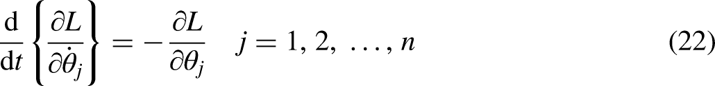
Derivation using Lagrange's method

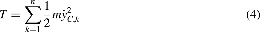
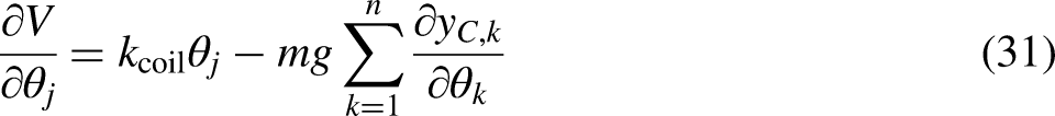
Another approach for deriving the equations of motion for a point mass model of a Slinky is the Lagrange method. The Lagrange method is less clear to a student engineer at the beginning of their university programme but is ideal for multi-body dynamic systems. The Lagrangian is defined to be

$$L=T-V$$

(3)

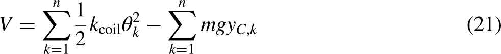
where T represents the kinetic energy of the system and V is the potential energy in the system, representing the elastic and gravitational potential energy. The Lagrangian has units of energy but is not the total energy in the system. For the point mass model, T and V are given as

$$T=\sum _{k=1}^n{\displaystyle \frac{1}{2}m{\dot{y}}_{C,k}^2}$$

(4)

$$V=\sum _{k=1}^n{\displaystyle \frac{1}{2}{k}_{pt}(y_{C,k}-y_{C,k-1}{)}^2-\sum _{k=1}^{n}mg{y}_{C,k}}$$

(5)

For k  =  1, y_C,k−1  =  0.

The equations of motion for the point mass model can be expressed as

$${\displaystyle \frac{\mathrm{d}}{\mathrm{d}t}\left\{{\displaystyle \frac{\mathrm{\partial }L}{\mathrm{\partial }{\dot{y}}_{C,j}}}\right\}=-{\displaystyle \frac{\mathrm{\partial }L}{\mathrm{\partial }{y}_{C,j}},j=1,2,\dots ,n}}$$

(6)

To derive the equations of motion in a form that can be solved using a numerical ODE solver, the terms above can be considered one by one.

$${\displaystyle \frac{\mathrm{d}}{\mathrm{d}t}\left\{{\displaystyle \frac{\mathrm{\partial }L}{\mathrm{\partial }{\dot{y}}_{C,j}}}\right\}=m{\ddot{y}}_{C,j}}$$

(7)

$$\begin{array}{rl}{\displaystyle \frac{\mathrm{\partial }L}{\mathrm{\partial }{y}_{C,j}}=}& k_{pt}(-y_{C,j+1}+2y_{C,j}-y_{C,j-1})-mg\\ y_{C,n+1}=& 0\end{array}$$

(8)

Substituting (7) and (8) into (6) and using matrix-vector notation is the same as (2).

Torsional spring model of a Slinky

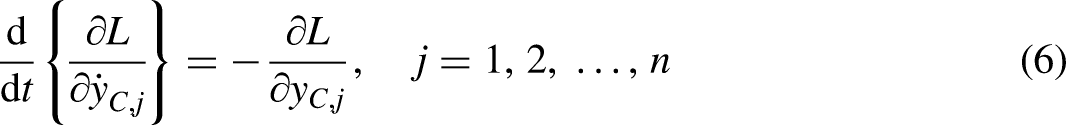
A Slinky is a continuous system that when held in a vertical orientation distorts the length of the Slinky under the action of gravity. In this section, the model for a Slinky based on the assumption that a Slinky can be represented as a series of half hoops connected to each other by torsion springs. For ease of reference, the model is referred to as the ‘torsion spring model’. Schematically the representation is shown in Figure 3.

Figure 3.

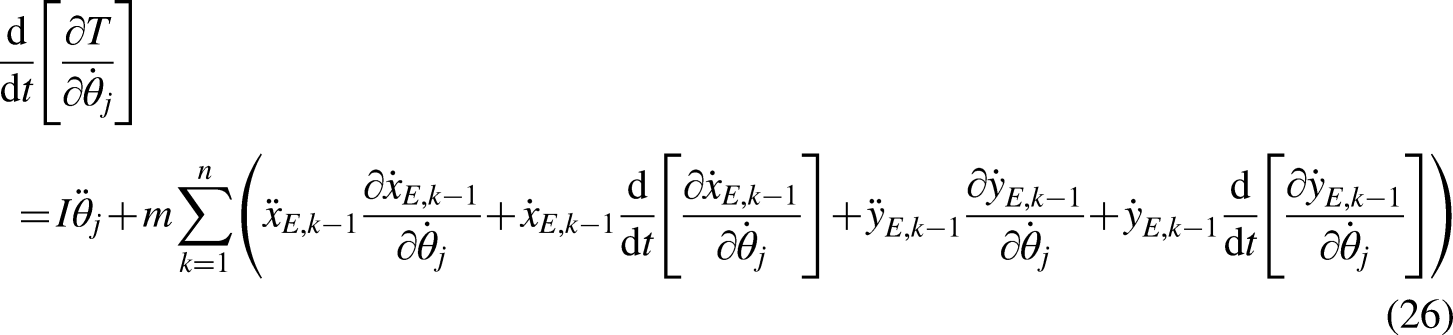
Schematic diagram of a torsion spring model of a Slinky.

In a Slinky, there is a constraint on the torsion angles, θ_k, defined in Figure 4 and introduced into the analysis below, (12). The constraint is that due to the coils in the Slinky the torsion angles cannot be less than a value based on the radius of the Slinky, R, and the thickness of a coil, Δ,

$${\tan }^{-1}{\displaystyle \frac{\mathrm{\Delta }}{2R}={\theta }_{\min }\le \theta }$$

(9)

Figure 4.

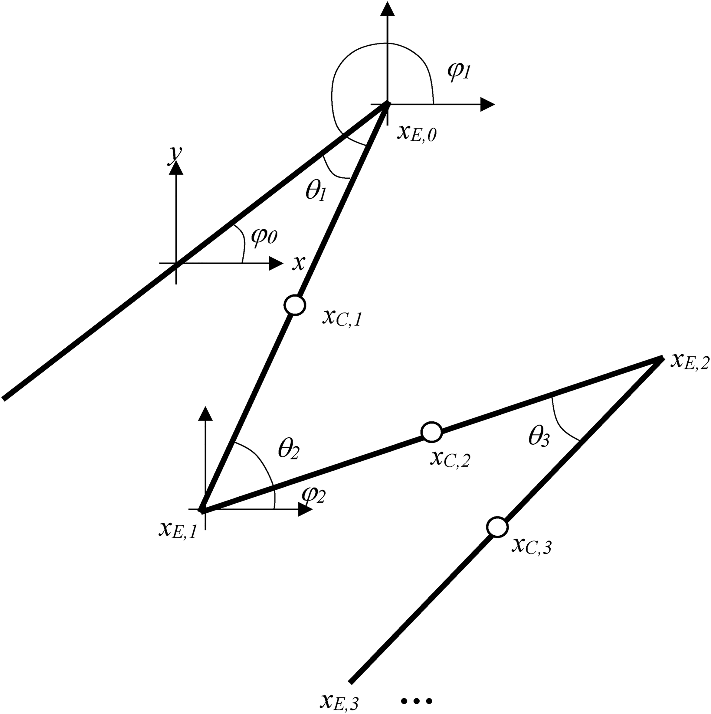
The kinematics of a torsion spring model of a Slinky.

This issue can be addressed by modelling a collision of two half coils as a purely plastic collision. In this article, this complication has not been implemented as the torsion spring model is sufficiently complicated to consider. In a later publication, it is planned to make the model more realistic such that (9) is satisfied.

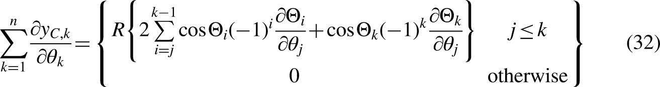
The kinematics of the torsion spring model

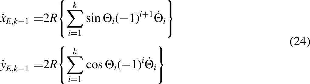
Before the equations of motion for the torsion spring model can be derived, the kinematics must be investigated. Figure 4 shows a schematic of the torsion spring model, looked at from the side. Therefore, each line in Figure 4 represents a half coil in the Slinky. Note for the derivation the angle φ₀ is set to zero. The end points of each half coil are given by the sequence:

$$\{{\mathit{x}}_{E,k}{\}}_{k=0}^n$$

(10)

The centre of mass of the half coils is labelled as follows:

$$\{{\mathit{x}}_{C,k}{\}}_{k=1}^n$$

(11)

The angles between the half hoops are labelled as the torsion angles:

$$\{{\theta }_k{\}}_{k=1}^n$$

(12)

and the angles the half coils make with the x-axis that allows the coordinates of the end points of the half coils to be specified are

$$\{{\phi }_k{\}}_{k=0}^n$$

(13)

The initial orientation of the surface the Slinky is fixed to is also specified in Figure 4. The slope angle orientation is denoted as φ₀. For φ₀ = 0, the Slinky is orientated to be suspended vertically down. For φ₀ = 180°, the Slinky is fixed to the top side of the surface.

An examination of Figure 4 shows the orientation angles, φ_k, and torsion angles, θ_k, are linked. The angle θ_k represents the angle between the half coils labelled as k − 1 and k.

$${\phi }_k=\left\{\begin{array}{cc}{\phi }_{k-1}+{\theta }_k+\pi & k\mathrm{is}\mathrm{odd}\\ {\phi }_{k-1}-{\theta }_k+\pi & k\mathrm{is}\mathrm{even}\end{array}\right\}$$

(14)

The parameters that will ultimately be treated as the independent variables of the equations of motion are labelled as the composite torsion angle defined as

$${\mathrm{\Theta }}_k={\phi }_0+\sum _{j=1}^k{\theta }_j(-1{)}^{j+1}$$

(15)

Using trigonometric addition formulae

$$\cos ({\mathrm{\Theta }}_k+\pi )=-\cos {\mathrm{\Theta }}_k$$

$$\sin ({\mathrm{\Theta }}_k+\pi )=-\sin {\mathrm{\Theta }}_k$$

it is possible to define the half coil edge point vectors and centre of mass point vectors as

$${\mathit{x}}_{E,k}={\mathit{x}}_{E,k-1}+2R\left(\begin{array}{c}\cos {\mathrm{\Theta }}_k\\ \sin {\mathrm{\Theta }}_k\end{array}\right)(-1{)}^k$$

(16)

$${\mathit{x}}_{C,k}={\mathit{x}}_{E,k-1}+R\left(\begin{array}{c}\cos {\mathrm{\Theta }}_k\\ \sin {\mathrm{\Theta }}_k\end{array}\right)(-1{)}^k$$

(17)

where R is the radius of the Slinky. The vertical coordinates of the centre of mass of the half coils can then be found using (16) and (17)

$$y_{C,k}=R\left(\sin {\mathrm{\Theta }}_0+2\sum _{i=1}^{k-1}\sin {\mathrm{\Theta }}_i{(-1)}^i+\sin {\mathrm{\Theta }}_k{(-1)}^k\right)$$

(18)

We can now derive the equations of motion for the torsion spring model of a Slinky.

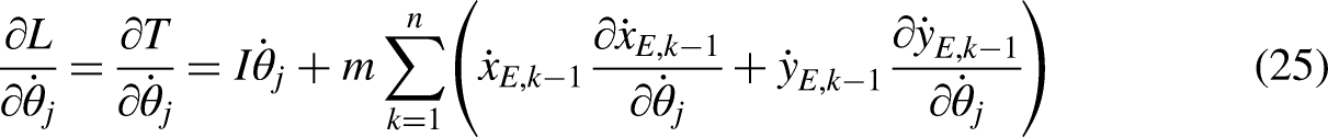
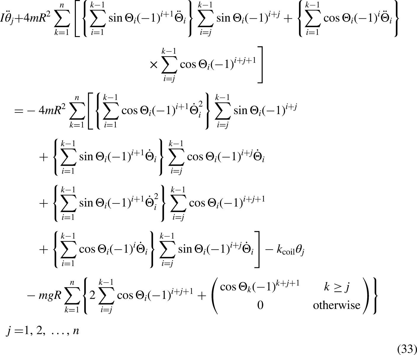
Derivation using Lagrange's method

The Lagrangian is as it was for the point mass model

$$L=T-V$$

(19)

where the terms T and V are defined as before. The Lagrangian for the torsion spring model of a Slinky is more complicated as each half hoop defined by its centre of mass, x _C,j has kinetic energy relating to its motion in the vertical and horizontal directions as well as rotational kinetic energy

$$T=\sum _{k=1}^n{\displaystyle \frac{1}{2}I{\dot{\theta }}_k^2+\sum _{k=1}^n{\displaystyle \frac{1}{2}m({\dot{x}}_{C,k}^2+{\dot{y}}_{C,k}^2)}}$$

(20)

$$V=\sum _{k=1}^n{\displaystyle \frac{1}{2}{k}_{\mathrm{coil}}{\theta }_k^2-\sum _{k=1}^{n}mg{y}_{C,k}}$$

(21)

This gives the generic equations of motion as

$${\displaystyle \frac{\mathrm{d}}{\mathrm{d}t}\left\{{\displaystyle \frac{\mathrm{\partial }L}{\mathrm{\partial }{\dot{\theta }}_j}}\right\}=-{\displaystyle \frac{\mathrm{\partial }L}{\mathrm{\partial }{\theta }_j}j=1,2,\dots ,n}}$$

(22)

All that remains is to express the equations of motion as functions of independent variables. The first step in this process is to note that the linear velocity at the centre of mass of the half hoop is the same as the linear velocity of the top edge

$${\dot{x}}_{C,k}={\dot{x}}_{E,k-1},{\dot{y}}_{C,k}={\dot{y}}_{E,k-1}$$

(23)

Using (16) the velocity components for the half hoop, k, is

$$\begin{array}{rl}{\dot{x}}_{E,k-1}=& 2R\left\{\sum _{i=1}^k\sin {\mathrm{\Theta }}_i{(-1)}^{i+1}{\dot{\mathrm{\Theta }}}_i\right\}\\ {\dot{y}}_{E,k-1}=& 2R\left\{\sum _{i=1}^k\cos {\mathrm{\Theta }}_i{(-1)}^i{\dot{\mathrm{\Theta }}}_i\right\}\end{array}$$

(24)

Using the chain rule and product differentiation, the derivatives in the generic equations of motion are as follows:

$${\displaystyle \frac{\mathrm{\partial }L}{\mathrm{\partial }{\dot{\theta }}_j}={\displaystyle \frac{\mathrm{\partial }T}{\mathrm{\partial }{\dot{\theta }}_j}=I{\dot{\theta }}_j+m\sum _{k=1}^n\left({\dot{x}}_{E,k-1}{\displaystyle \frac{\mathrm{\partial }{\dot{x}}_{E,k-1}}{\mathrm{\partial }{\dot{\theta }}_j}+{\dot{y}}_{E,k-1}{\displaystyle \frac{\mathrm{\partial }{\dot{y}}_{E,k-1}}{\mathrm{\partial }{\dot{\theta }}_j}}}\right)}}$$

(25)

$$\begin{array}{rl}& {\displaystyle \frac{\mathrm{d}}{\mathrm{d}t}\left[{\displaystyle \frac{\mathrm{\partial }T}{\mathrm{\partial }{\dot{\theta }}_j}}\right]}\\ & =I{\ddot{\theta }}_j+m\sum _{k=1}^n\left({\ddot{x}}_{E,k-1}{\displaystyle \frac{\mathrm{\partial }{\dot{x}}_{E,k-1}}{\mathrm{\partial }{\dot{\theta }}_j}+{\dot{x}}_{E,k-1}{\displaystyle \frac{\mathrm{d}}{\mathrm{d}t}\left[{\displaystyle \frac{\mathrm{\partial }{\dot{x}}_{E,k-1}}{\mathrm{\partial }{\dot{\theta }}_j}}\right]+{\ddot{y}}_{E,k-1}{\displaystyle \frac{\mathrm{\partial }{\dot{y}}_{E,k-1}}{\mathrm{\partial }{\dot{\theta }}_j}+{\dot{y}}_{E,k-1}{\displaystyle \frac{\mathrm{d}}{\mathrm{d}t}\left[{\displaystyle \frac{\mathrm{\partial }{\dot{y}}_{E,k-1}}{\mathrm{\partial }{\dot{\theta }}_j}}\right]}}}}\right)\end{array}$$

(26)

$${\displaystyle \frac{\mathrm{\partial }{\dot{x}}_{E,k-1}}{\mathrm{\partial }{\dot{\theta }}_j}=2R\left\{\sum _{i=j}^{k-1}\sin {\mathrm{\Theta }}_i{(-1)}^{i+1}{\displaystyle \frac{\mathrm{\partial }{\dot{\mathrm{\Theta }}}_i}{\mathrm{\partial }{\dot{\theta }}_j}}\right\}=2R\left\{\sum _{i=j}^{k-1}\sin {\mathrm{\Theta }}_i{(-1)}^{i+j}\right\}}$$

(27)

$${\displaystyle \frac{\mathrm{d}}{\mathrm{d}t}\left[{\displaystyle \frac{\mathrm{\partial }{\dot{x}}_{E,k-1}}{\mathrm{\partial }{\dot{\theta }}_j}}\right]=2R\left\{\sum _{i=j}^{k-1}\cos {\mathrm{\Theta }}_i{(-1)}^{i+j}{\dot{\mathrm{\Theta }}}_i\right\}}$$

(28)

$${\displaystyle \frac{\mathrm{\partial }{\dot{y}}_{E,k-1}}{\mathrm{\partial }{\dot{\theta }}_j}=2R\left\{\sum _{i=j}^{k-1}\cos {\mathrm{\Theta }}_i{(-1)}^{i+j+1}\right\}}$$

(29)

$${\displaystyle \frac{\mathrm{d}}{\mathrm{d}t}\left[{\displaystyle \frac{\mathrm{\partial }{\dot{y}}_{E,k-1}}{\mathrm{\partial }{\dot{\theta }}_j}}\right]=2R\left\{\sum _{i=j}^{k-1}\sin {\mathrm{\Theta }}_i{(-1)}^{i+j}{\dot{\mathrm{\Theta }}}_i\right\}}$$

(30)

where the mass of a half coil is denoted m and the mass moment of inertia for a half coil, modelled as a half hoop is, I. Applying the chain rule and product differentiation to the potential energy term, V, in (21)

$${\displaystyle \frac{\mathrm{\partial }V}{\mathrm{\partial }{\theta }_j}=k_{\mathrm{coil}}{\theta }_j-mg\sum _{k=1}^n{\displaystyle \frac{\mathrm{\partial }{y}_{C,k}}{\mathrm{\partial }{\theta }_k}}}$$

(31)

$$\sum _{k=1}^n{\displaystyle \frac{\mathrm{\partial }{y}_{C,k}}{\mathrm{\partial }{\theta }_k}=\left\{\begin{array}{cc}R\left\{2\sum _{i=j}^{k-1}\cos {\mathrm{\Theta }}_i{(-1)}^i{\displaystyle \frac{\mathrm{\partial }{\mathrm{\Theta }}_i}{\mathrm{\partial }{\theta }_j}+\cos {\mathrm{\Theta }}_k{(-1)}^k{\displaystyle \frac{\mathrm{\partial }{\mathrm{\Theta }}_k}{\mathrm{\partial }{\theta }_j}}}\right\}& j\le k\\ 0& \mathrm{otherwise}\end{array}\right\}}$$

(32)

Note k_coil denotes the torsion spring constant. Substituting equations (26)–(32) into (22) and rearranging all second-order derivative terms to be on the left-hand side gives the following system of ODEs:

$$\begin{array}{rl}I{\ddot{\theta }}_j+& 4m{R}^2\sum _{k=1}^n[\left\{\sum _{i=1}^{k-1}\sin {\mathrm{\Theta }}_i{(-1)}^{i+1}{\ddot{\mathrm{\Theta }}}_i\right\}\sum _{i=j}^{k-1}\sin {\mathrm{\Theta }}_i{(-1)}^{i+j}+\left\{\sum _{i=1}^{k-1}\cos {\mathrm{\Theta }}_i{(-1)}^i{\ddot{\mathrm{\Theta }}}_i\right\}\\ & \times \sum _{i=j}^{k-1}\cos {\mathrm{\Theta }}_i{(-1)}^{i+j+1}]\\ =& -4m{R}^2\sum _{k=1}^n[\left\{\sum _{i=1}^{k-1}\cos {\mathrm{\Theta }}_i{(-1)}^{i+1}{\dot{\mathrm{\Theta }}}_i^2\right\}\sum _{i=j}^{k-1}\sin {\mathrm{\Theta }}_i{(-1)}^{i+j}\\ & +\left\{\sum _{i=1}^{k-1}\sin {\mathrm{\Theta }}_i{(-1)}^{i+1}{\dot{\mathrm{\Theta }}}_i\right\}\sum _{i=j}^{k-1}\cos {\mathrm{\Theta }}_i(-1{)}^{i+j}{\dot{\mathrm{\Theta }}}_i\\ & +\left\{\sum _{i=1}^{k-1}\sin {\mathrm{\Theta }}_i{(-1)}^{i+1}{\dot{\mathrm{\Theta }}}_i^2\right\}\sum _{i=j}^{k-1}\cos {\mathrm{\Theta }}_i(-1{)}^{i+j+1}\\ & +\left\{\sum _{i=1}^{k-1}\cos {\mathrm{\Theta }}_i{(-1)}^i{\dot{\mathrm{\Theta }}}_i\right\}\sum _{i=j}^{k-1}\sin {\mathrm{\Theta }}_i{(-1)}^{i+j}{\dot{\mathrm{\Theta }}}_i]-k_{\mathrm{coil}}{\theta }_j\\ & -mgR\sum _{k=1}^n\left\{2\sum _{i=j}^{k-1}\cos {\mathrm{\Theta }}_i{(-1)}^{i+j+1}+\left(\begin{array}{cc}\cos {\mathrm{\Theta }}_k{(-1)}^{k+j+1}& k\ge j\\ 0& \mathrm{otherwise}\end{array}\right)\right\}\\ j=& 1,2,\dots ,n\end{array}$$

(33)

This is a complicated system of second-order differential equations. It is not clear what are the independent variables. From the definition of the system, the torsion angles, (12), are the candidate independent variables. An inspection of (33) would suggest the composite torsion angles, (15), are a better choice. Using the following mapping from the composite torsion angles to the torsion angles, it is possible to close system (33) using the composite torsion angles as the independent variables

$${\theta }_j=\left\{\begin{array}{cc}{\mathrm{\Theta }}_1& j=1\\ ({\mathrm{\Theta }}_j-{\mathrm{\Theta }}_{j-1}){(-1)}^{j+1}& j>1\end{array}\right\}$$

(34)

The system of differential equations, (33), is complicated but not impossible to implement in an ODE numerical solver. For convenience (33) is referred to in the remainder of the paper as follows:

$$B\ddot{\mathbf{\Theta }}=f(\mathbf{\Theta },\dot{\mathbf{\Theta }})$$

(35)

The different mathematical processes such as product differentiation, chain differentiation and the manipulation of systems of differential equations are familiar to a final-year undergraduate mechanical engineering student the model is well beyond even the more able student. The value of the model is something that theoretically reproduces the behaviour of a Slinky and can be compared with the point mass model. In addition, the torsion spring model has the potential to reproduce a range of Slinky dynamic behaviour not found in the point mass model.

Torsion spring model for n  =  1, 2 and 3

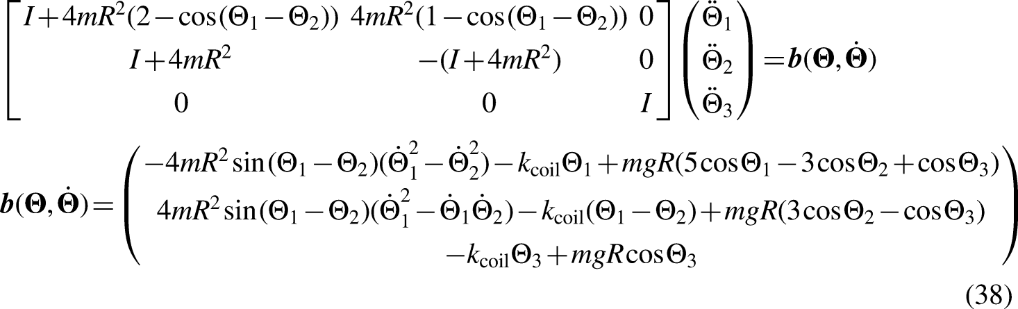
The general system of equations describing the motion of a Slinky with n half coils, (33), is very complicated to implement. It is useful to consider the system for small values of n. In this subsection, the torsion spring model is presented with 1 half coil (n  =  1), 1 coil (n  =  2) and 1.5 coils (n  =  3). This is of interest as these models can be used for verification of the computer implementation of (33). They also show that it is not possible to identify a simpler representation of the mathematical basis of the torsion model of a Slinky than (33).

The simplest case is a single half coil (n  =  1). The equation of motion is given as follows:

$$I{\ddot{\mathrm{\Theta }}}_1+k_{\mathrm{coil}}{\mathrm{\Theta }}_1=mgR\cos {\mathrm{\Theta }}_1$$

(36)

Note this can also be derived by taking a moment at x _E,0 and applying Newton's second law for a rotating system. The case for n  =  2 is given below:

$$\left[\begin{array}{cc}I+4m{R}^2& 0\\ I& -I\end{array}\right]\left(\begin{array}{c}{\ddot{\mathrm{\Theta }}}_1\\ {\ddot{\mathrm{\Theta }}}_2\end{array}\right)=\left(\begin{array}{c}-k_{\mathrm{coil}}{\mathrm{\Theta }}_1+mgR(3\cos {\mathrm{\Theta }}_1-\cos {\mathrm{\Theta }}_2)\\ -k_{\mathrm{coil}}{\mathrm{\Theta }}_2+mgR(\cos {\mathrm{\Theta }}_1-\cos {\mathrm{\Theta }}_2)\end{array}\right)$$

(37)

The case for n  =  3 is given below:

$$\begin{array}{rl}& \left[\begin{array}{ccc}I+4m{R}^2(2-\cos ({\mathrm{\Theta }}_1-{\mathrm{\Theta }}_2))& 4m{R}^2(1-\cos ({\mathrm{\Theta }}_1-{\mathrm{\Theta }}_2))& 0\\ I+4m{R}^2& -(I+4m{R}^2)& 0\\ 0& 0& I\end{array}\right]\left(\begin{array}{c}{\ddot{\mathrm{\Theta }}}_1\\ {\ddot{\mathrm{\Theta }}}_2\\ {\ddot{\mathrm{\Theta }}}_3\end{array}\right)=\mathit{b}(\mathbf{\Theta },\dot{\mathbf{\Theta }})\\ & \mathit{b}(\mathbf{\Theta },\dot{\mathbf{\Theta }})=\left(\begin{array}{c}-4m{R}^2\sin ({\mathrm{\Theta }}_1-{\mathrm{\Theta }}_2)({\dot{\mathrm{\Theta }}}_1^2-{\dot{\mathrm{\Theta }}}_2^2)-k_{\mathrm{coil}}{\mathrm{\Theta }}_1+mgR(5\cos {\mathrm{\Theta }}_1-3\cos {\mathrm{\Theta }}_2+\cos {\mathrm{\Theta }}_3)\\ 4m{R}^2\sin ({\mathrm{\Theta }}_1-{\mathrm{\Theta }}_2)({\dot{\mathrm{\Theta }}}_1^2-{\dot{\mathrm{\Theta }}}_1{\dot{\mathrm{\Theta }}}_2)-k_{\mathrm{coil}}({\mathrm{\Theta }}_1-{\mathrm{\Theta }}_2)+mgR(3\cos {\mathrm{\Theta }}_2-\cos {\mathrm{\Theta }}_3)\\ -k_{\mathrm{coil}}{\mathrm{\Theta }}_3+mgR\cos {\mathrm{\Theta }}_3\end{array}\right)\end{array}$$

(38)

Note the complexity of the system of ODEs grows rapidly with an increasing number of half coils. Identifying a structure that simplifies the system for the general case to something simpler than (33) is not possible.

Converting a second-order ODE system to a first-order ODE system

To solve the system, (33) numerically it is required to convert it to a first-order system. This is necessary as it is required that the system is expressed in the form:

$$\dot{\mathit{Y}}=\mathit{f}(t,\mathit{Y})$$

(39)

Even if the right-hand side has no dependency on time, t. This is easily done by creating a vector of independent variables

$$\mathit{Y}=\left(\begin{array}{c}{\mathrm{\Theta }}_1\\ \begin{array}{c}{\mathrm{\Theta }}_2\\ \dots \\ \begin{array}{c}{\mathrm{\Theta }}_n\\ \begin{array}{c}{\dot{\mathrm{\Theta }}}_1\\ {\dot{\mathrm{\Theta }}}_2\\ \begin{array}{c}\dots \\ {\dot{\mathrm{\Theta }}}_n\end{array}\end{array}\end{array}\end{array}\end{array}\right)$$

(40)

Then, the equivalent of (33) or in its more concise representation, (35) is of the form:

$$\left[\begin{array}{cc}{I}_n& 0\\ 0& B\end{array}\right]\dot{\mathit{Y}}=\left(\begin{array}{c}\begin{array}{c}{Y}_{n+1}\\ Y_{n+2}\end{array}\\ \begin{array}{c}\dots \\ \begin{array}{c}{Y}_{n2}\\ f_1(\mathit{Y})\\ \begin{array}{c}{f}_2(\mathit{Y})\\ \dots \\ f_n(\mathit{Y})\end{array}\end{array}\end{array}\end{array}\right)$$

(41)

Vertical motion of a Slinky

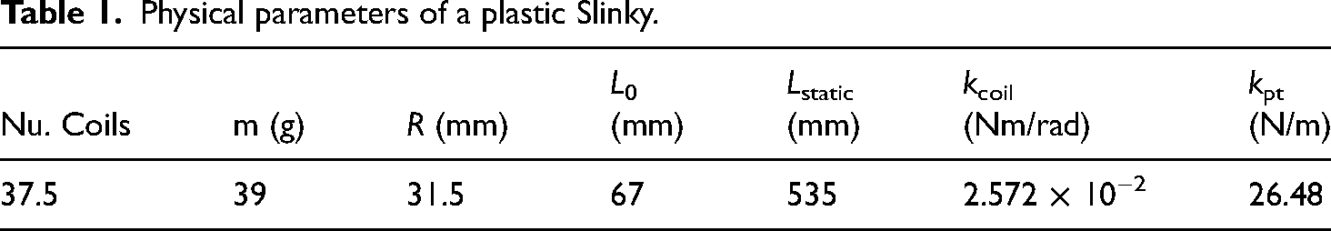
Having derived the respective mathematical models, we can investigate their respective predictions of the dynamic behaviour of a Slinky. Attention will be restricted to a plastic Slinky with the parameters given in Table 1 unless stated otherwise.

Table 1.

Physical parameters of a plastic Slinky.

Nu. Coils	m (g)	R (mm)	L0(mm)	Lstatic(mm)	kcoil(Nm/rad)	kpt(N/m)
37.5	39	31.5	67	535	2.572  ×  10−2	26.48

Point mass model

The first case considered is the simulation of a plastic Slinky with 15 half coils, n  =  15. The initial condition is a stationary Slinky with the initial vertical heights of the point masses located at the origin. The vertical locations of all point masses as a function of time for the first 2 s of simulation time is shown in Figure 5. The first point of note is that the point mass trajectories change with increasing time. Why this might be is discussed in the context of the torsion spring model as it is a more obvious issue for this model. Similar to Prez, ¹¹ the point masses close to the origin follow a triangular trajectory, compared with point masses located near the end of the Slinky that have a more harmonic trajectory. This is likely to be a property of the model rather than the Slinky. This will be discussed further later. For the plastic Slinky with n  =  15, the point mass model prediction of amplitude and period is 0.0463 m and 0.275 s.

Figure 5.

Point mass model, n  =  15, prediction of point mass locations for i  =  1, 2,…, 15.

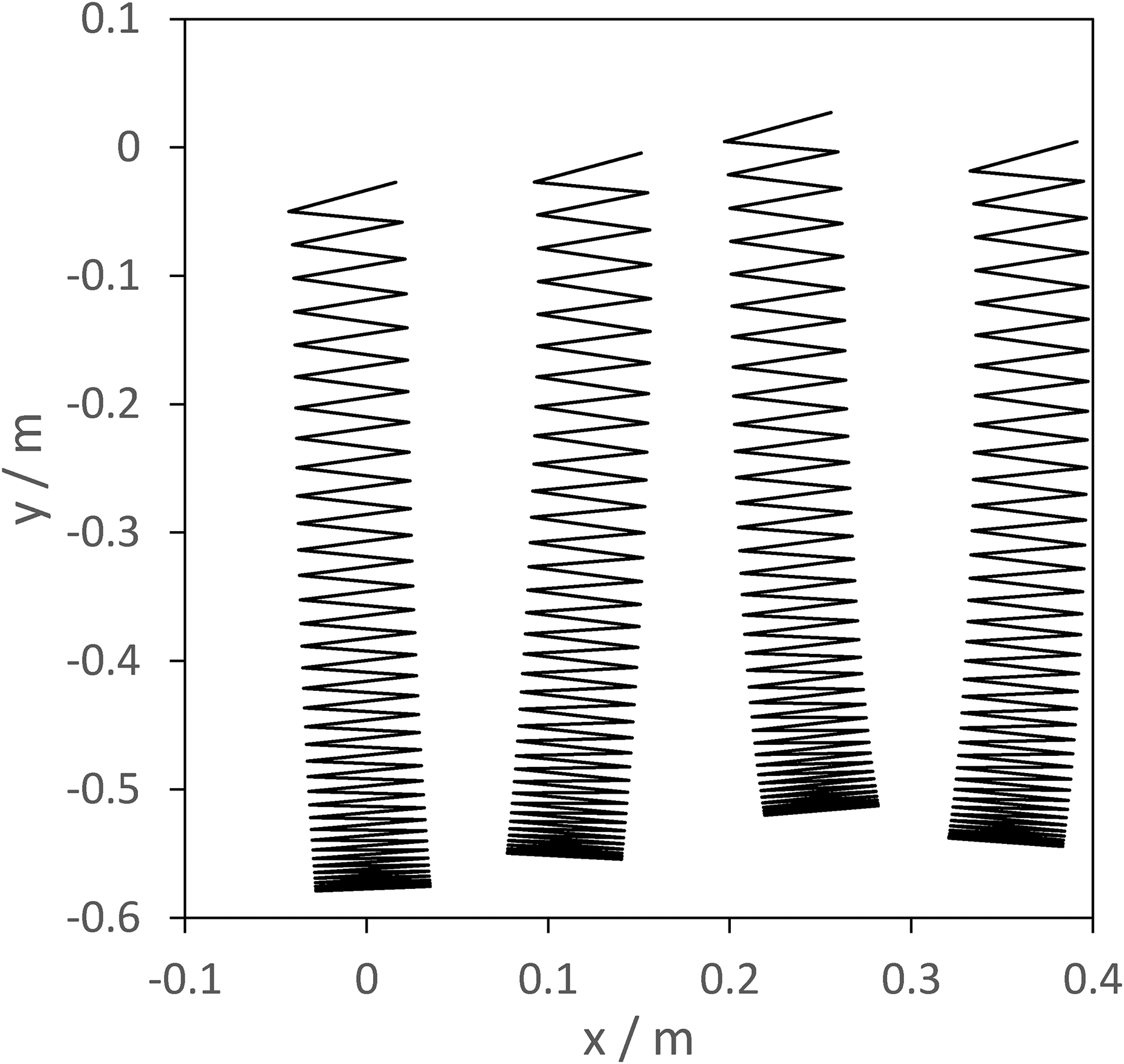
The second application of the point mass model is the simulation of a plastic Slinky with 75 half coils, n  =  75. The initial condition is the same as above, the Slinky is initially stationary with all point masses located at the origin. In Figure 6, the location of the first five masses closest to the origin and the last point mass in the Slinky are plotted for the first 4 s of simulation time. The qualitative behaviour of the Slinky is similar to the n  =  15 Slinky shown in Figure 5. The amplitude and period of the Slinky are 1.1 m and 1.34 s.

Figure 6.

Point mass model, n  =  75, prediction of point mass locations for i  =  1, 2, 3, 4, 5 and 75.

In the limit of an infinite number of point masses, the point mass model, (2), tends to the wave equation ¹¹ showing that for the wave equation the period of a wave satisfies the expression:

$$T=\sqrt{{\displaystyle \frac{32(L_{\mathrm{static}}-L_0)}{-g}}}$$

(42)

For the plastic Slinky with n  =  75, this gives a period of 1.24 s. The relative difference between the point mass model and the wave equation is approximately 8%. This is interesting but it should be appreciated this is not a validation of the point mass model as it is one theory being compared against another ¹¹ demonstrating a similar level of agreement with experimental data for a plastic Slinky with a similar set of physical parameters. As an aside ¹¹ state that the period, (42), does not depend on the mass of the Slinky or the spring constants, however, the length of a vertically orientated Slinky stretched under its own weight, L_static, does depend on the mass of the Slinky and the spring constant.

Torsion spring model

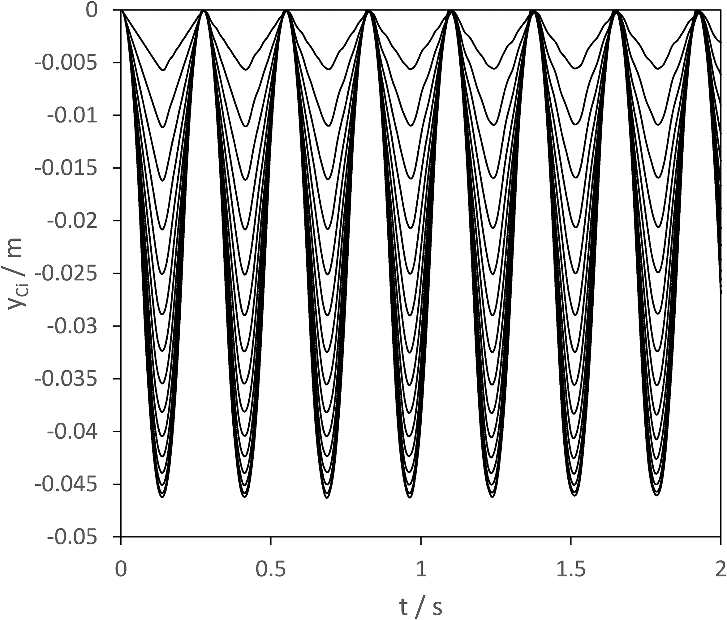
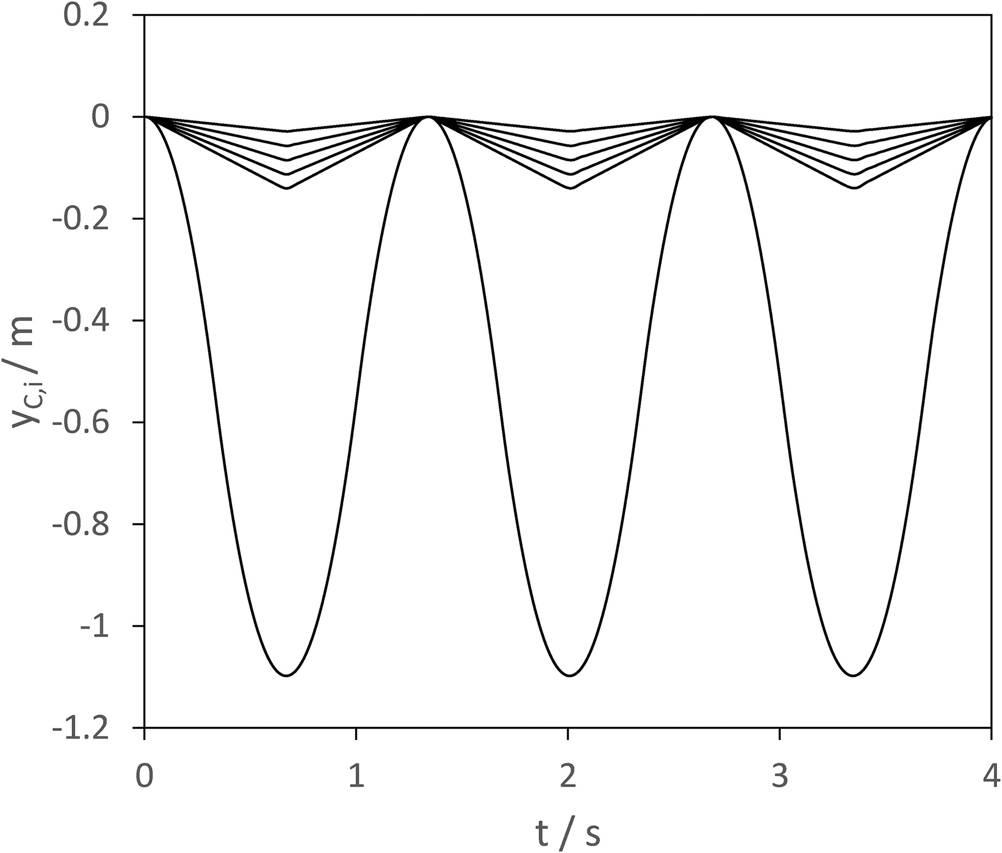
The torsion spring model of a Slinky is initially applied to the plastic Slinky with n  =  15, similar to the first simulation using the point mass model. The initial conditions are of a Slinky at rest with all torsion angles set to zero, the equivalent of all half coil centres of masses are located at the origin. The vertical locations of all centres of masses are plotted for a simulation time of 2 s in Figure 7. In Figure 7, the torsion spring model prediction should be compared with Figure 5, the equivalent plot for the point mass model. As time progresses there is a reduction in uniformity of the oscillation in the Slinky half coil centre of mass locations. This will be addressed further below. From Figure 7, it is clear that the constraint on the torsion angles is violated when the Slinky is close to its initial condition

$${\theta }_j=0\mathrm{rad},j=1,2,\dots ,15$$

Figure 7.

Torsion spring model, n  =  15, prediction of the centre of mass locations for i  =  1, 2,…, 15.

Over the simulation time of 2 s the trajectory of the Slinky changes from a purely vertical up-down motion to a more irregular motion. It is not clear if this is an issue to do with the numerical methods employed or a property of the model. Overall, the period and amplitude remain reasonably steady. The amplitude and period are approximately 0.0466 m and 0.271 s. Comparing these with the equivalent point mass predictions, the relative differences are 0.6% and 1.5% in amplitude and period, respectively.

Both the point mass model and torsion spring model of a Slinky are conservative. When a numerical method is applied to the solution of a conservative ODE system round-off error introduces an energy imbalance. If the energy imbalance on average introduces spurious energy into the system, the numerical solution tends to blow up. If on average the energy imbalance removes energy from the system, this makes it a dissipative model and the long-time solution tends towards the equilibrium state of the Slinky.

The total energy of the system is

$$E=\sum _{k=1}^n{\displaystyle \frac{1}{2}I{\dot{\theta }}_k^2+\sum _{k=1}^n{\displaystyle \frac{1}{2}m({\dot{x}}_{C,k}^2+{\dot{y}}_{C,k}^2)+\sum _{k=1}^n{\displaystyle \frac{1}{2}{k}_{\mathrm{coil}}{\theta }_k^2-\sum _{k=1}^{n}mg{y}_{C,k}}}}$$

(43)

In Figure 8, the maximum and minimum energy imbalance is plotted against the number of half coils. In all simulations, the initial condition is a stationary Slinky with the torsion angles set to zero. The maximum and minimum energy imbalance is calculated for the first 2 s of simulation time. From Figure 8 it is clear that for n ≤ 15, the energy imbalance to the resolution of the figure is negligible. Beyond n = 15, the difference in maximum and minimum energy imbalance increases, indicating that the trajectory of the model either blows up or behaves like a dissipative system. From numerical experiments, the solutions for times significantly beyond 2 s are not possible for n > 15. This is disappointing as for most Slinkies there are more than 15 half coils.

Figure 8.

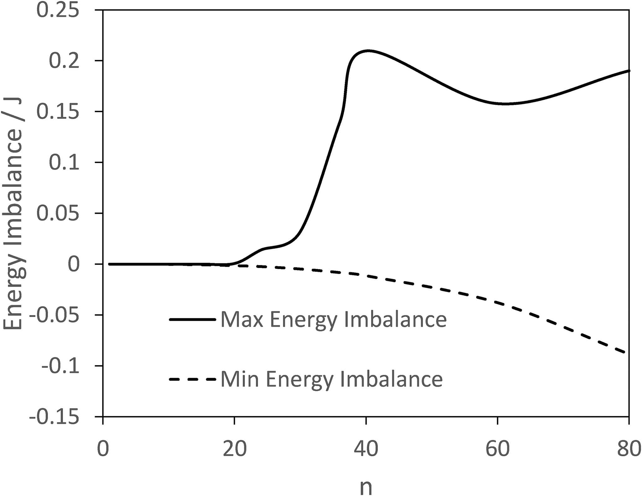
Torsion spring model, max/min energy imbalance in the system calculated over 2 s of simulation time.

Fortunately, a real Slinky is a dissipative system. Work is done on a real Slinky by drag force and elastic deformation of the spring is not ideal. The drag force is likely to be small relative to the nonideal elastic deformation of a Slinky as a mechanism for energy loss. In this paper, nonideal elastic deformation is modelled by changing the equations of motion to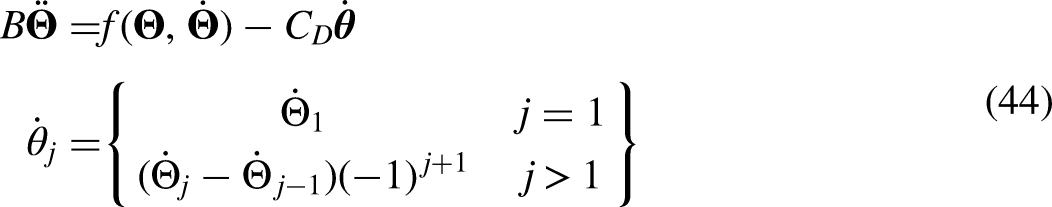

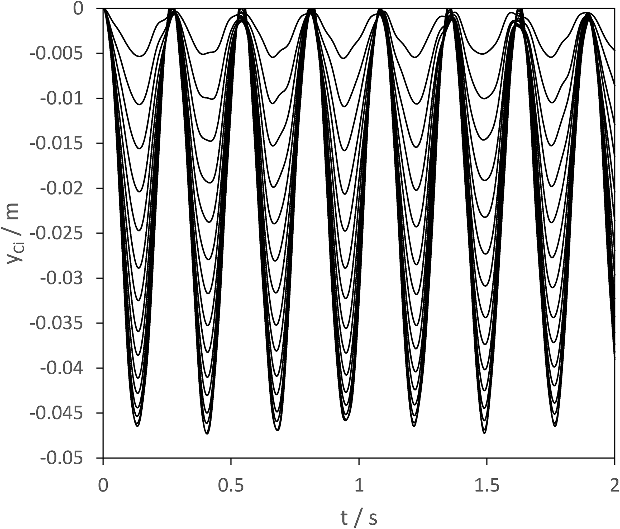
$$\begin{array}{rl}B\ddot{\mathbf{\Theta }}=& f(\mathbf{\Theta },\dot{\mathbf{\Theta }})-C_D\dot{\mathit{\theta }}\\ {\dot{\theta }}_j=& \left\{\begin{array}{cc}{\dot{\mathrm{\Theta }}}_1& j=1\\ ({\dot{\mathrm{\Theta }}}_j-{\dot{\mathrm{\Theta }}}_{j-1}){(-1)}^{j+1}& j>1\end{array}\right\}\end{array}$$

(44)

This is the simplest way of introducing dissipation into the system and has been used successfully to model frictional losses at a pivot. ¹⁸ Within the context of the torsion spring model, it can be thought of as frictional loss within the torsional springs. Note the constant C_D is a parameter being used to make the numerical solution of the equations of motion slightly dissipative and hence numerically stable.

Figure 9 shows an equivalent simulation to that shown in Figure 7 for a Slinky with n  =  15. The difference is that the predicted Slinky trajectory in Figure 9 is calculated using (44) with a small level of energy dissipation, C_D = 10⁻⁵. Comparing Figures 7 and 9, the dissipative Slinky simulation shown in Figure 9 is more realistic than for the conservative Slinky simulation shown in Figure 7. In Figure 9, the oscillations for early time are more uniform. For a latter time, the dissipative term, (44), reduces the amplitude of the Slinky oscillations as for a long-time the simulation will converge to an equilibrium state.

Figure 9.

Torsion spring model including dissipation (C_D  =  10⁻⁵), n  =  15, prediction of centre of mass locations for i  =  1, 2,…, 15.

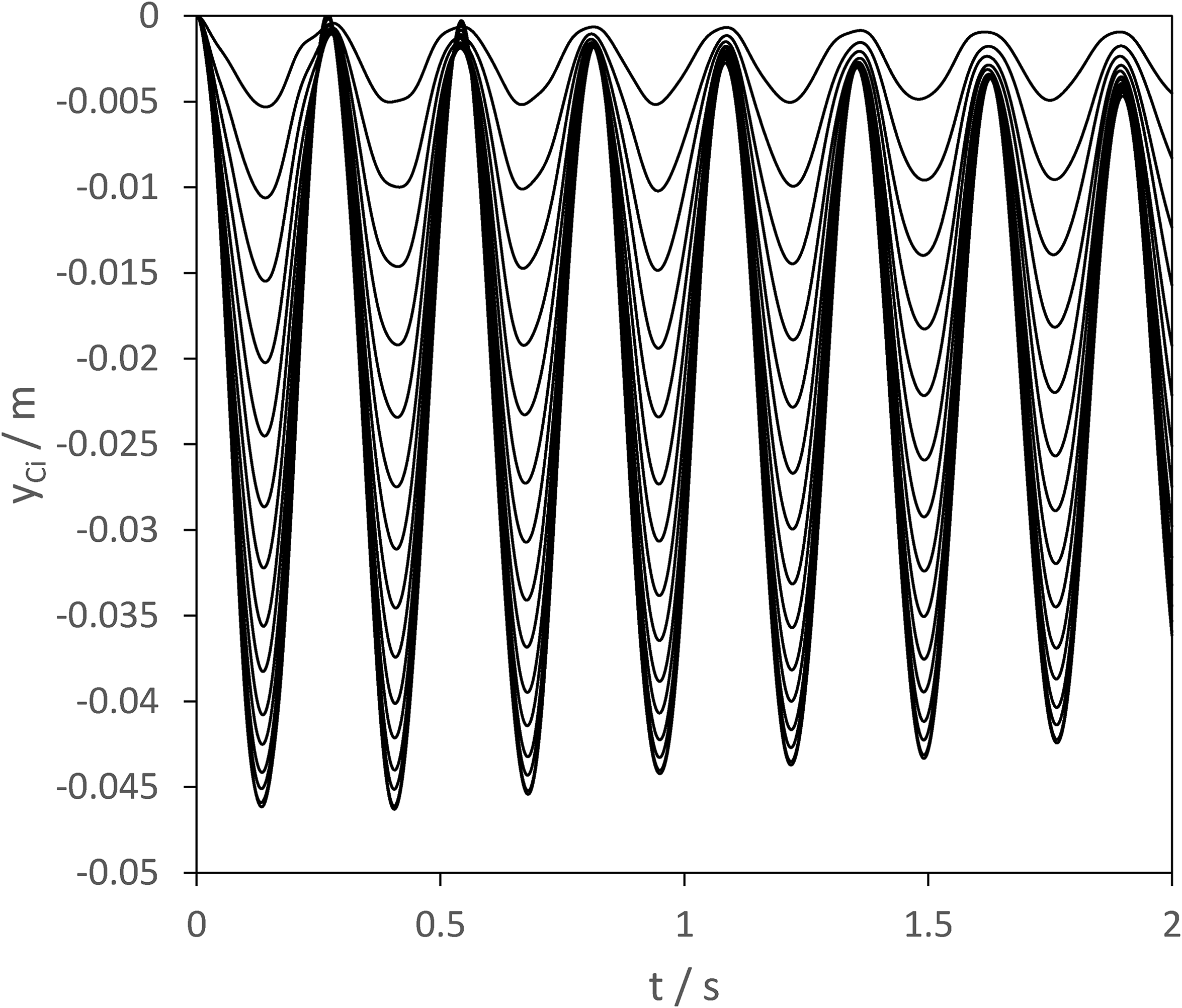
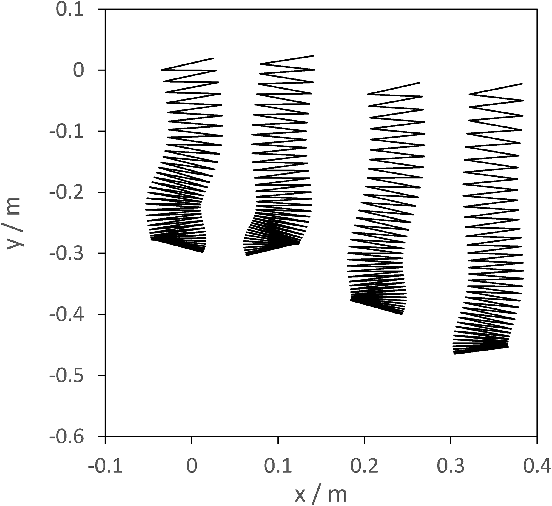
Introducing dissipation into the ODE system equations of motion, (44), it is possible to simulate Slinkies with a reasonable number of half coils. Returning to the n  =  75 half coil simulation of the point mass model, see Figure 6, the initial condition is a stationary Slinky with the centre of mass of all half coils located at the origin. The dissipation constant is set to C_D  =  3  ×  10⁻⁴. Figure 10 shows the location of the centre of mass of the half coils, j  =  1, 2,…,5 and j  =  75. On comparing Figures 6 and 10, the period is similar for both Slinky models. For the first cycle of the torsion spring model simulation, see Figure 10, is similar to the point mass model, Figure 6. Using the data in Figure 10, the torsion spring model prediction of the first cycle amplitude is 1.03 m and the period is 1.3 s. These values are close to those calculated using the point mass model.

Figure 10.

Torsion spring model including dissipation (C_D  =  3  ×  10⁻⁴), n  =  75, prediction of the centre of mass locations for i  =  1, 2, 3, 4, 5 and 75.

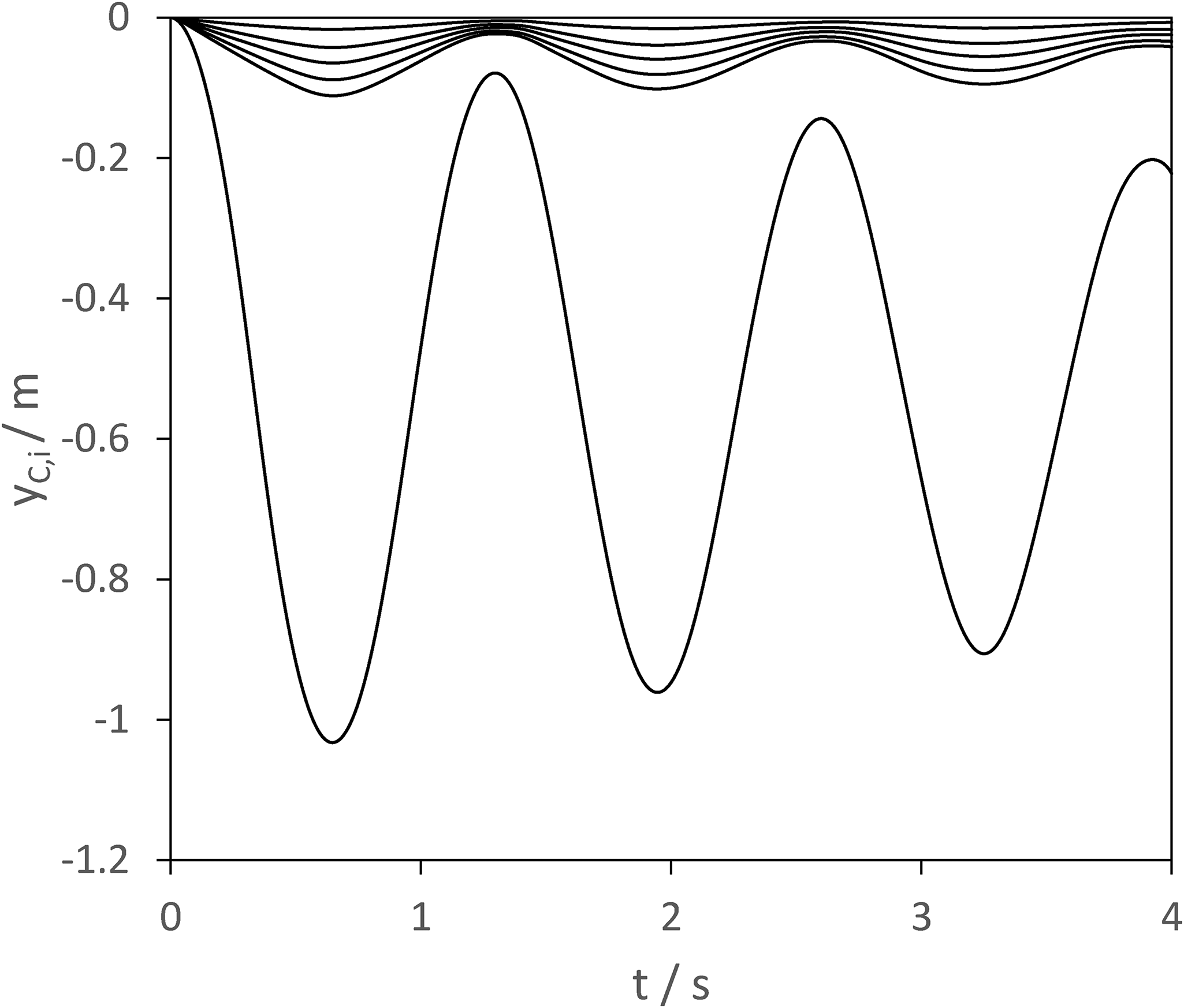
Investigating the trajectory of the centre of masses of the half coils is of interest but does not really show the overall dynamic behaviour of a Slinky very well. An animation of a Slinky would be ideal but the best that can be done is to look at the Slinky for different time slices. Figure 11 shows a characterisation of a Slinky's motion n  =  75 Slinky at four time slices, t  =  0.3, 0.6, 0.9 and 1.2 s, calculated using the dissipative torsion angle model, (C_D  =  3  ×  10⁻⁴). For clarity, a shift in the x coordinate of the Slinky for t  =  0.6, 0.9 and 1.2 s is introduced. For example

$$x_{\mathrm{shift}}(t=0.3)=x+0.12$$

Figure 11.

Simulation of torsion spring model including dissipation, n  =  75, for t  =  0.3, 0.6, 0.9 and 1.2 s.

The vertical motion is clear as well as some lateral motion. The lateral motion is subtle and to the knowledge of the author has not been identified in previous experimental investigations. Something that is more obvious is that the Slinky half coils can be separated into two sets. The two sets can be defined as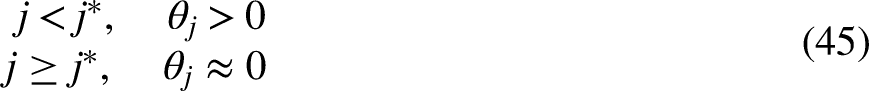

$$\begin{array}{c}j<j*,{\theta }_j>0\\ j\ge j*,{\theta }_j\approx 0\end{array}$$

(45)

For $j\ge j*$ , the acceleration and tension in the torsion angles are too great to be overcome by the weight of the Slinky below $y_{C,j*}$ . Note j* changes during the cycle of the Slinky motion.

For the amplitude and period, the predictions of the point mass model and torsion spring model are similar. One interesting result is the distortion in the Slinky for the torsion spring model is nonlinear. Intuitively you would expect the torsion angles to increase from the bottom of the Slinky towards the top. This is because the self-weight of the Slinky increases as you increase the vertical component of the centre of mass of the half coils. This property for the point mass model is true. Consider Figure 7, a prediction of the location of the centre of masses as a function of time for n  =  15 using the torsion spring model, for t  =  0.14 s. It is subtle but it can be identified that

$$|y_{C,1}|<|y_{C,2}-y_{C,1}|$$

(46)

For the point mass model, the equivalent figure is Figure 5. For the point mass model, the opposite is the case and in fact the property is

$$|y_{C,1}|>|y_{C,2}-y_{C,1}|>|y_{C,3}-y_{C,2}|>\dots$$

(47)

To investigate this further the property

$$max|y_{C,j}-y_{C,j-1}|$$

(48)

for the simulations, with n  =  75, shown in Figures 7 and 10, (48) is plotted against half hoop/point mass index in Figure 12. The point mass model exhibits the inequality property, (47). For the torsion spring model, the situation is more complicated in that for j  =  1, 2,…, 6 the behaviour is not monotonic. The largest spring distortion occurring for j  =  2, not j  =  1. Why is this? The answer is not obvious. Possibly one important difference between the point mass model and the torsion spring model is that the fixed point of the torsion spring model is not on the line of action of the weight vectors, however, how this leads to this nonlinear behaviour is not obvious. When the Slinky is in static equilibrium with a vertical orientation the same nonlinear behaviour is exhibited. ²⁵ Further work to explain this nonintuitive result is required.

Figure 12.

Maximum difference between centres of mass for n  =  75, 0 < t < 1 s.

Forcing a Slinky

As stated above, due to the structure of a Slinky, the torsion angles are required to satisfy the inequality constraint (9). In this paper, the torsion angle constraint is not imposed, the Slinky dynamics are restricted such that the torsion angles are positive or at worst are very small negative values for a limited range of simulation time. This limits the range of initial conditions that can be investigated.

Natural frequencies and the small angle approximation

Whenever considering a forced dynamical system the natural frequencies of the system are key to understanding the influence of the forcing frequency of the forcing function. To calculate the natural frequencies, the torsion spring model, (33), is linearised by introducing the small angle approximation

$${\mathrm{\Theta }}_k\approx 0$$

(49)

such that

$$\cos {\mathrm{\Theta }}_k\approx 1$$

(50)

$$\sin {\mathrm{\Theta }}_k\approx {\mathrm{\Theta }}_k$$

(51)

Substituting the above approximations into (33) gives the approximate system

$$\begin{array}{rl}I{\ddot{\theta }}_j+& 4m{R}^2\sum _{k=1}^n\left[\left\{\sum _{i=1}^{k-1}{(-1)}^i{\ddot{\mathrm{\Theta }}}_i\right\}\sum _{i=j}^{k-1}{(-1)}^{i+j+1}\right]\\ =& -k_{\mathrm{coil}}{\theta }_j-mgR\sum _{k=1}^n\left\{2\sum _{i=j}^{k-1}{(-1)}^{i+j+1}+\left(\begin{array}{cc}{(-1)}^{k+j+1}& k\ge j\\ 0& \mathrm{otherwise}\end{array}\right)\right\}\\ {\theta }_j=& \left\{\begin{array}{cc}{\mathrm{\Theta }}_1& j=1\\ ({\mathrm{\Theta }}_j-{\mathrm{\Theta }}_{j-1}){(-1)}^{j+1}& j>1\end{array}\right\}\end{array}$$

(52)

As a model for simulating the behaviour of a Slinky it is not a very useful approximation but consider the homogenous part of (52)

$$M_{\mathrm{coil}}\ddot{\mathbf{\Theta }}+K_{\mathrm{coil}}\mathbf{\Theta }=0$$

(53)

then the natural frequencies can be calculated. Where the mass matrix, M_coil, is defined by the left-hand side of (52) and the stiffness matrix, K_coil, is as follows:

$$K_{\mathrm{coil}}=\left[\begin{array}{ccc}{k}_{\mathrm{coil}}& 0& \begin{array}{cc}\cdots & \begin{array}{cc}& 0\end{array}\end{array}\\ k_{\mathrm{coil}}& -k_{\mathrm{coil}}& \begin{array}{ccc}0& \cdots & 0\end{array}\\ \begin{array}{c}0\\ 0\end{array}& \begin{array}{c}\ddots \\ \cdots \end{array}& \begin{array}{ccc}\begin{array}{c}\ddots \\ 0\end{array}& \begin{array}{c}0\\ k_{\mathrm{coil}}{(-1)}^n\end{array}& \begin{array}{c}⋮\\ k_{\mathrm{coil}}{(-1)}^{n+1}\end{array}\end{array}\end{array}\right]$$

(54)

The eigenvalues of the homogeneous system are

$${\lambda }_i=\mathrm{eigenvalues}\mathrm{of}(M_{\mathrm{coil}}^{\text{-}1}{K}_{\mathrm{coil}})i=1,2,\dots ,n$$

(55)

The natural frequencies are

$${\omega }_i=\sqrt{{\lambda }_i},i=1,2,\dots ,n$$

(56)

A similar analysis of the point mass model gives natural frequencies as

$${\lambda }_i=\mathrm{eigenvalues}\mathrm{of}\left(-{\displaystyle \frac{k_{pt}}{m}A}\right),i=1,2,\dots ,n$$

(57)

$${\omega }_i=\sqrt{{\lambda }_i},i=1,2,\dots ,n$$

(58)

No forcing of the point mass model is considered here but it is of interest to compare the natural frequencies of the torsion spring model and the point mass model. Figure 13 shows the natural frequencies for the n  =  75 plastic Slinky for the torsion spring model and the point mass model. The natural frequencies of the two models are very different implying that for a given forcing frequency the dynamic behaviour of the two models will likely be very different. The second point of note is the torsion spring model natural frequencies are arranged in pairs except for ω₇₅ the highest natural frequency of the system. Some numerical experiments on the torsion spring model suggest that if n is even then there exist n different natural frequencies. If n is odd then there are (n − 1)/2  +  1 different natural frequencies. For the torsion spring model applied to the plastic Slinky with n  =  75, the first three natural frequencies are

$${\omega }_1={\omega }_2=4.6904{\mathrm{s}}^{-1},{\omega }_3=13.964{\mathrm{s}}^{-1}$$

Figure 13.

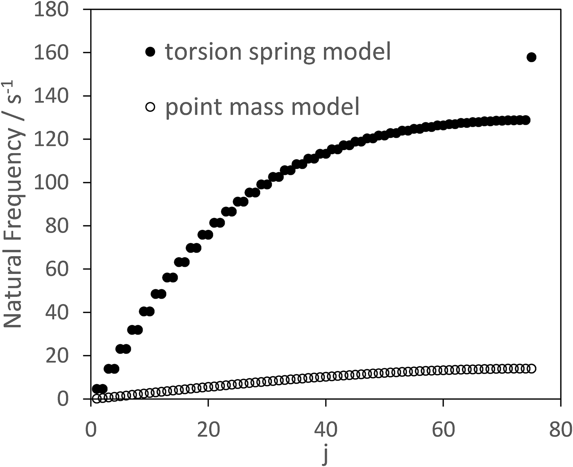
Natural frequencies of the point mass model and torsion spring model for n  =  75.

Angular forcing

In this section, the torsion spring model is extended to investigate angular forcing. The Slinky is forced by making the initial orientation, φ₀ time dependent. The forcing term takes the form

$${\phi }_0(t)=A_{\phi }\sin (\mathrm{\Omega }t)$$

(59)

This modifies the equations of motion to be

$$B\ddot{\mathbf{\Theta }}=f(\mathbf{\Theta },\dot{\mathbf{\Theta }})-C_D\dot{\mathit{\theta }}+\mathit{f}({\phi }_0,{\dot{\phi }}_0,{\ddot{\phi }}_0)$$

(60)

$$\mathit{f}({\phi }_0,{\dot{\phi }}_0,{\ddot{\phi }}_0)=\left(\begin{array}{c}\begin{array}{c}{f}_1\\ f_2\end{array}\\ \begin{array}{c}⋮\\ f_n\end{array}\end{array}\right)$$

$$\begin{array}{rl}{f}_j({\phi }_0,{\dot{\phi }}_0,{\ddot{\phi }}_0)=& 2m{R}^2\sum _{k=1}^n[\{\cos {\phi }_0{\dot{\phi }}_0^2+\sin {\phi }_0{\ddot{\phi }}_0\}\sum _{i=j}^{k-1}\sin {\mathrm{\Theta }}_i{(-1)}^{i+j}\\ & +\{\sin {\phi }_0{\dot{\phi }}_0\}\sum _{i=j}^{k-1}\cos {\mathrm{\Theta }}_i(-1{)}^{i+j}{\dot{\mathrm{\Theta }}}_i\\ & +\{\sin {\phi }_0{\dot{\phi }}_0^2-\cos {\phi }_0{\ddot{\phi }}_0\}\sum _{i=j}^{k-1}\cos {\mathrm{\Theta }}_i(-1{)}^{i+j+1}\\ & -\{\cos {\phi }_0{\dot{\phi }}_0\}\sum _{i=j}^{k-1}\sin {\mathrm{\Theta }}_i{(-1)}^{i+j}{\dot{\mathrm{\Theta }}}_i],j=1,2,\dots ,n\end{array}$$

Forcing the initial angle of orientation, φ₀, is chosen as it is straightforward to specify initial conditions and the parameters, A_φ and Ω such that the condition that the torsion angles are not negative is possible without directly imposing the constraint.

For the two simulations discussed in this section, the initial condition is specified to be a plastic Slinky, n  =  75, in static vertical equilibrium. The forcing amplitude is fixed to be A_φ=π/3 rad. The forcing frequency is given two values, Ω = 4.69 s⁻¹ and Ω=13.96 s⁻¹. These two values are chosen as they are just below the first and second distinct natural frequencies.

The period of the forcing function is

$$T={\displaystyle \frac{2\pi }{\mathrm{\Omega }}}$$

(61)

In Figure 14, four time slices of the simulation with Ω = 4.69 s⁻¹ are shown. For a forcing frequency of 4.69 s⁻¹, the forcing period is T  =  1.34 s. The time for each time slice is t  =  5 s, t  =  5  +  0.25T, 5  +  0.5T and t  =  5  +  0.75T. Similar to Figure 11, for clarity, for each time slice, an origin shift in the x-direction of Δx  =  0.12 is applied. From the figure, it can be inferred that the movement of the Slinky in response to the forcing term is a swaying side-to-side motion. Any vertical motion is more to do with the angular forcing at the top rather than a change in the torsion angles of the Slinky.

Figure 14.

Forced torsion spring model, φ₀  =  0, A_φ = π/3 rad, Ω = 4.69 s⁻¹, t  =  5, 5.33, 5.67 and 6 s.

In Figure 15, four time slices of the simulation with Ω = 13.96 s⁻¹ are shown. The initial condition and simulation parameters are the same for this simulation as the previous angular forcing simulation except the forcing frequency is increased. The key difference is the forcing frequency is above the first distinct natural frequency. A value just below the second distinct frequency is chosen as it takes less simulation time to see the effect of the higher forcing frequency. For this simulation, the forcing period is T  =  0.45 s. As expected, the behaviour of the Slinky is very different to the other forced Slinky. Rather than swaying from side to side, there is a ‘wobble’ introduced into the Slinky's motion with a significant vertical motion of the Slinky.

Figure 15.

Forced torsion spring model, φ₀  =  0, A_φ = π/3 rad, Ω = 13.96 s⁻¹, t  =  5, 5.11, 5.23 and 5.34 s.

Conclusion

In this paper, the Lagrange method is applied to derive the equations of motion for a model of a Slinky based on point masses and a model based on half hoops connected by torsion springs. The point mass model is relatively straightforward and can be used to simulate some of the interesting dynamic behaviour of Slinkies. The torsion spring model is much more complicated to derive and solve than the point mass model.

As a conservative model, the torsion spring models numerical solution is limited to very small Slinkies $(n\le 15)$ . If energy dissipation is introduced to stabilise the numerical solution of the torsion spring model, then Slinkies with a realistic number of coils can be modelled. For unforced motion, the point mass model and the torsion spring model predict the amplitude and frequency of oscillations of a Slinky reasonably closely. No simulations of the point mass model for a forced Slinky are considered, given the natural frequencies are very different to the torsion spring model's natural frequencies. It is not likely that the two models would produce similar Slinky trajectories for the same forcing frequency.

The potential advantage of the torsion spring model is with some minor modification it can simulate at least qualitatively the fall range of dynamic behaviour of a Slinky; propagation of longitudinal and translational waves, pseudo levitation, and propagation down a stair.

To address some of the phenomena discussed above, the torsion spring model needs to include the physical constraint (9), that the torsion angles have a lower bound. This could be done by imposing conservation of momentum during a plastic impact of two adjacent half coils. There is a rich vein of research into the dynamics of a Slinky that can be explored using a modified torsion spring model. It is planned to introduce the above extension of the torsion spring model when considering other aspects of the dynamics of Slinkies. This would require detection of the violation of constraint (9), termination of the ODE numerical solver algorithm, calculation of the new angular velocities of the torsion angles to conserve momentum followed by the reactivation of the ODE solver algorithm with the modified initial conditions to continue the simulation.