Studying transient heat transfer in a cylindrical pin fin with radiation and convection

Abstract

A simple experimental fin device was used to develop a laboratory procedure for undergraduate engineering students, in order to enhance their understanding of the transfer of thermal energy. This experiment exposes the student to several important concepts, namely one-dimensional, time-dependent heat transfer in extended surfaces by conduction, convection and radiation. In a few simple steps, students have the opportunity to compare the measured to the predicted temperature profiles obtained at different times using an analytical complex solution and to calculate convective and radiative heat coefficients, such as the relative predominance of convection heat transfer with respect to radiation.

Introduction

Heat transfer enhancement is an active and important field of engineering, since any increases in the effectiveness of transferred heat could result in considerable technical advantages and cost savings. The interest in such problems stems from their importance in many engineering applications such as thermal design of heat exchangers, air conditioning, convective heat loss from solar collectors, and the cooling of electronic or mechanical components. When additional metal strips, called fins, are attached to ordinary heat-transfer surfaces, they extend the surface available for heat transfer between the solid and the surrounding fluid . ¹ While the finned surface increases the total transmission of heat, its influence as a surface is treated differently from simple conduction and convection problems, and its mathematical description can be complicated. It is important for engineers to understand the principles of heat transfer, and to be able to use the rate equations that govern the mechanisms of transmission of heat (i.e., conduction, convection and radiation). However, the majority of students perceive its mathematical representation as a difficult subject. Heat-fin experiments are important didactical resources to show practical applications of sophisticated mathematical techniques. The integration of the present experiment into undergraduate courses would allow students to familiarize themselves with this technique and enhance their understanding of extended surfaces.

Here we present a simple experiment that illustrates transient heat conduction in a cylindrical fin involving combined convection and radiation effects. In this experiment, the fin is assumed to be insulated at the end and the heat-flow is intended to be one dimensional. Under transient conditions, students record the time-dependent temperatures of the fin at several positions along its length and compare the measured temperature profile with the analytical solution at regular intervals of time. The convective and radiative heat transfer coefficients are also evaluated from the measured temperature profile, as well as the time needed to achieve the steady-state conditions. In addition, students could validate the dominance of convective heat transfer at low surface temperatures, and the dominance of radiation heat transfer at high surface temperatures.

Other papers describe similar experiments involving heat conduction in a fin. In some cases, experiments are conducted under steady-state conditions .^2–4 In other cases, radiation or convection is neglected ^5–8 or boundary conditions differ from those used in this work. As such, the equation required to carry out our experiment is not evident to find in books usually employed in undergraduate heat transfer courses.

The experiment described further on is part of a series of six different laboratories that students accomplish in the “Mechanical laboratory II” course. As a course typically taken in the sixth trimester of their curriculum, students review topics taught in the fluids/heat transfer stem of the mechanical engineering program, as well as learn new experimental techniques. It is a one credit course taught as 1.5 h of lecture and 21 h of laboratory (3.5 h for each experiment). A laboratory handout is given at the beginning of the course, well before the laboratory period, which outlines the fundamental topics and references as a review. The main objectives of this course are: i) learning to use the procedures, skills, and modern engineering tools necessary for engineering practice, including experimental approaches and techniques, data-analysis methods, and engineering measurement systems; ii) learning how to evaluate and interpret experimental data using their knowledge of physics and engineering principles; iii) learning how to present experimental results by writing a professional report at the end of each laboratory.

Methodology

Experimental apparatus and procedure

The experimental apparatus is relatively simple and inexpensive (see Fig. 1). A 10 mm diameter brass rod $(k=92W/m\cdot K;\alpha =2.2\times {10}^{-5}{m}^2/s)$ of approximately 350 mm effective length is mounted horizontally on a short stand. The rod is heated at one end and maintained at a constant temperature by an electrical heater inside an insulated housing in direct contact with the brass rod. The remaining exposed length is allowed to cool by natural convection and radiation, and the tip of the rod is insulated. The temperature of the base is controlled using a variable-voltage transformer, while the surface temperature is recorded by eight K-type thermocouples attached to the rod in order to minimise errors from conduction effects located at 50 mm intervals along the rod. An additional thermocouple is mounted on the unit to record the ambient air temperature. The type K (nickel-chromium) is the most common type of thermocouple. It's inexpensive, accurate, reliable, and has a wide temperature range. An AT4116 Multi-Channel Temperature Meter is used to read temperature values along the length of the fin every 5 s with an accuracy of $\pm {1.1}^{\circ }C$ , as reported by the manufacturer. Finally, the rod is coated with a heat resistant matte black paint in order to provide a constant radiant emissivity close to 1.

Figure 1.

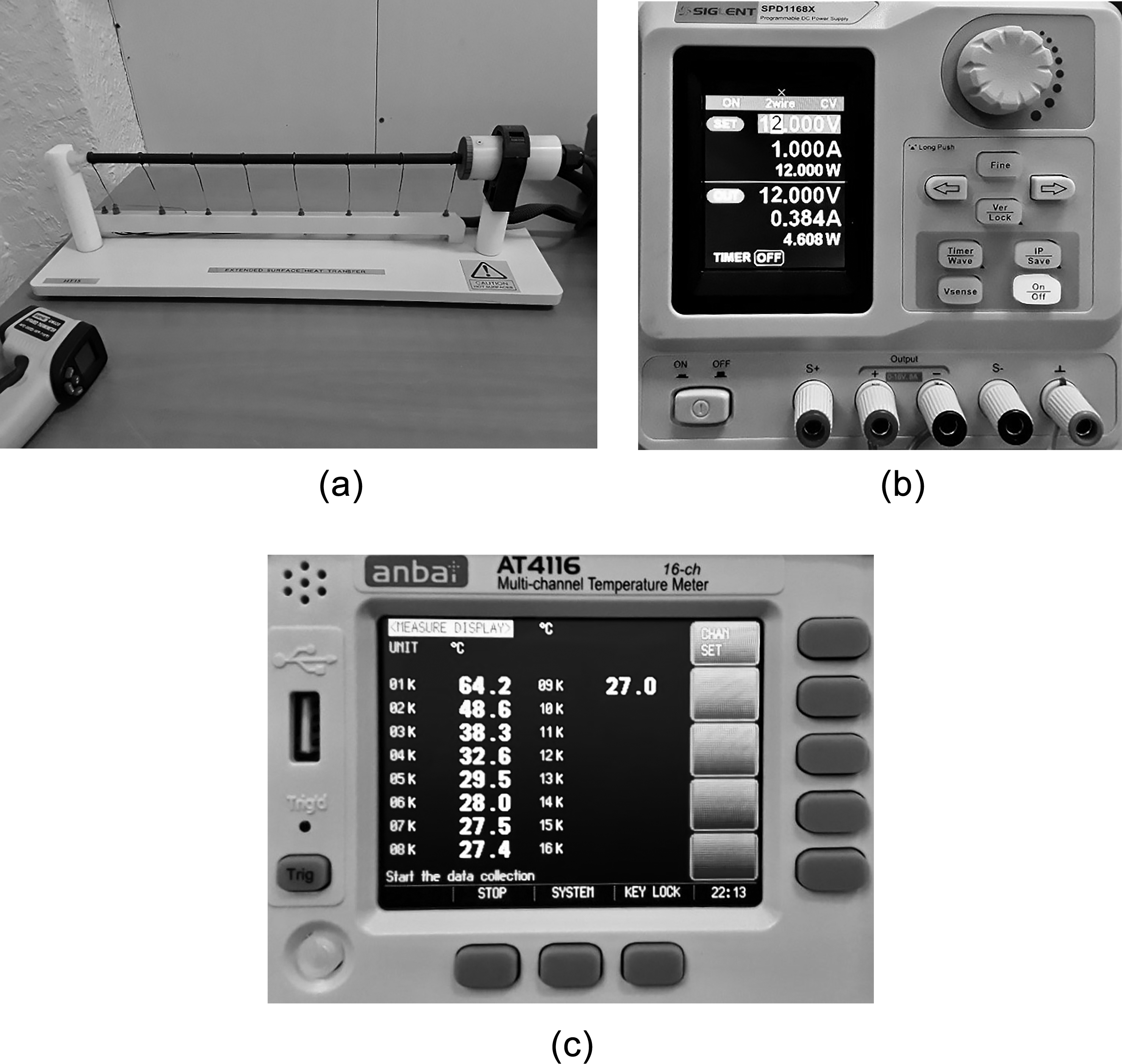
(a to c) Extended surface experimental apparatus: (a) the cylindrical brass pin fin connected to the thermocouples; (b) SPD1168X siglent programmable dc power supply connected to the heater; (c) anba AT4116 multi-channel temperature meter.

The experimental procedure is simple and straightforward to carry out. First, students turn on the voltage controller and increase the voltage to 9 V. Second, they record the axial temperature distribution (T1 to T8) and ambient air temperature T_a every 5 min until all temperatures are stable. Once readings have been completed, the voltage may be reduced to zero to allow the rod to cool. If time permits, they may carry out the experiment a second time increasing the voltage to 16 V and repeating the above readings until steady-state conditions are reached once again. The duration of the entire experiment is approximately 3 h. However, in order to verify our model, we repeated measurements for 9 V, 12 V, 14 V and 16 V, recording the axial temperature profile at different times. A comparison between experimental data and our model is presented and discussed in the Results and discussion section.

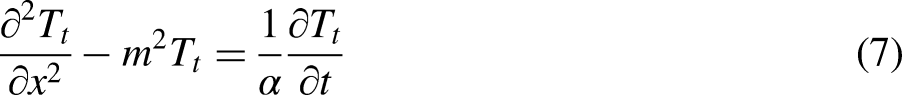
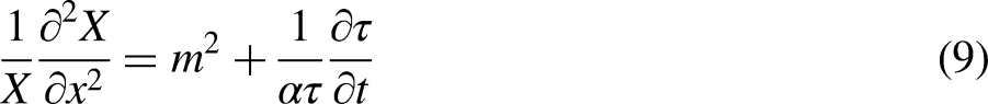
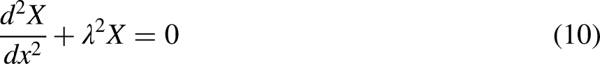
Mathematical formulation

Consider a straight cylindrical fin of constant cross-sectional area A, perimeter of the cross-section P, and length L as shown in Fig.1. The fin has a thermal conductivity k and a thermal diffusivity $\alpha$ . At time $t>0$ , the base of the fin, initially in thermal equilibrium with the surroundings at temperature $T_a$ , undergoes a change in temperature from $T_a$ to $T_b$ in one step while its tip remains insulated. For one-dimensional transient conduction in the fin, the energy equation may be written as

$${\displaystyle \frac{{\mathrm{\partial }}^{2}T}{\mathrm{\partial }{x}^2}-m^2(T-T_a)={\displaystyle \frac{1}{\alpha }{\displaystyle \frac{\mathrm{\partial }T}{\mathrm{\partial }t}}}}$$

(1)where x is measured from the base of the fin, and $m=\sqrt{{\overline{h}}^{*}P/k{A}_c}$ is called the fin parameter. The combined effect of radiation and convection is taken into account in ${\overline{h}}^{*}$ parameter, whose meaning will be detailed later on.

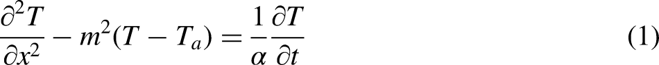
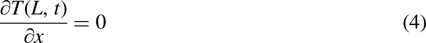
The initial and boundary conditions are

$$T(x,0)=T_a$$

(2)

$$T(0,t)=T_b$$

(3)

$${\displaystyle \frac{\mathrm{\partial }T(L,t)}{\mathrm{\partial }x}=0}$$

(4)We know that at infinite time the system attains a steady state temperature profile $T_s(x)$ . We then may write

$$T(x,t)=T_s(x)+T_t(x,t)$$

(5)where $T_t(x,t)$ is the transient part of the solution, which fades out as time goes to infinity. Equation (5) may be unfamiliar to students, but the concept is simple. Substitution of this expression into the original differential equation allows us to separate the steady-state fin equation,

$${\displaystyle \frac{{\mathrm{\partial }}^2{T}_s}{\mathrm{\partial }{x}^2}-m^2(T_s-T_a)=0}$$

(6)from the equation for the transient term,

$${\displaystyle \frac{{\mathrm{\partial }}^2{T}_t}{\mathrm{\partial }{x}^2}-m^2{T}_t={\displaystyle \frac{1}{\alpha }{\displaystyle \frac{\mathrm{\partial }{T}_t}{\mathrm{\partial }t}}}}$$

(7)The solution to Equation (6) is $T_s=T_a+c_1{e}^{mx}+c_2{e}^{-mx}$ , where $c_1$ and $c_2$ are coefficients to be determined by the boundary conditions, Equations. (3) and (4). The final solution is

$$T_s=T_a+(T_b-T_a){\displaystyle \frac{\cosh m(L-x)}{\cosh mL}}$$

(8)The transient solution may be found by the technique of separation of variables, in which we assume a solution of the form $T_t(x,t)=X(x)\tau (t)$ , where $X(x)$ and $\tau (t)$ are functions to be determined. Substitution of this trial solution into Equation (7) and then division by the product $X\tau$ gives

$${\displaystyle \frac{1}{X}{\displaystyle \frac{{\mathrm{\partial }}^{2}X}{\mathrm{\partial }{x}^2}=m^2+{\displaystyle \frac{1}{\alpha \tau }{\displaystyle \frac{\mathrm{\partial }\tau }{\mathrm{\partial }t}}}}}$$

(9)The left side is a function of t alone, and the right side is a function of x alone. This means that both sides must equal a constant. We have chosen to designate the constant as $-{\lambda }^2$ . We could use $\lambda$ or $+{\lambda }^2$ as well, but those choices would make the subsequent mathematics somewhat more complicated. Equation (9) can then be separated into two equations

$${\displaystyle \frac{d^{2}X}{d{x}^2}+{\lambda }^{2}X=0}$$

(10)

$${\displaystyle \frac{d\tau }{dt}=-\alpha \tau (m^2+{\lambda }^2)}$$

(11)These equations have the following solutions $\tau (t)=c{e}^{-\alpha (m^2+{\lambda }^2)t}$ and $X(x)=c_1\cos \lambda (L-x)+c_2\sin \lambda (L-x)$ where $c,c_1$ and $c_2$ are unknown coefficients, which must satisfy the boundary conditions given in Equations (3) and (4). Equation (4) is satisfied if $X(x)$ has the form $\cos \lambda (L-x)$ and Equation (3) requires $c_1\cos \lambda L$ to be zero. This will be true if $c_2=0$ or $\cos \lambda L=0$ . The first choice would lead to $X=0$ for all x, and that would be physically unacceptable. Therefore, we make the second choice, which leads to the eigenvalues ${\lambda }_n=\pm (n+(1/2))(\pi /L)$ . We note that the exponentials and cosines for n have the same values as those for $-(n+1)$ , so that the terms with negative indices combine with those with positive indices. Hence, the solution becomes

$$T_t(x,t)=\sum _{n=0}^{\mathrm{\infty }}{c}_n{e}^{-\alpha (m^2+{\lambda }_n^2)t}\cos {\lambda }_n(L-x)$$

(12)with ${\lambda }_n=\pm (n+(1/2))(\pi /L)$ . According to the initial condition, $T_t(x,0)=T_a-T_s(x)$ , so that

$$-(T_b-T_a){\displaystyle \frac{\cosh m(L-x)}{\cosh mL}=\sum _{n=0}^{\mathrm{\infty }}{c}_n\cos \left(n+{\displaystyle \frac{1}{2}}\right){\displaystyle \frac{\pi }{L}(L-x)}}$$

(13)To determine all values of $c_n$ , we multiply both sides of the equation by $\cos (m+(1/2))\frac{\pi }{L}(L-x)$ , where m is an integer, and then integrate from $x=0$ to $x=L$ , thus:

$$\begin{array}{rl}-& (T_b-T_a)\underset{0}{\overset{L}{\int }}{\displaystyle \frac{\cosh m(L-x)}{\cosh mL}\cos \left(m+{\displaystyle \frac{1}{2}}\right){\displaystyle \frac{\pi }{L}(L-x)dx}}\\ & =\sum _{n=0}^{\mathrm{\infty }}{c}_n\underset{0}{\overset{L}{\int }}\cos \left(n+{\displaystyle \frac{1}{2}}\right){\displaystyle \frac{\pi }{L}\cos \left(m+{\displaystyle \frac{1}{2}}\right){\displaystyle \frac{\pi }{L}(L-x)dx}}\end{array}$$

(14)The left side gives $-(T_b-T_a)\cdot (mL\sinh mL\cos {\lambda }_{n}L+{\lambda }_{n}L\cosh mL\sin {\lambda }_{n}L)/L\cosh mL(m^2+{\lambda }_n^2)$ ; the integral on the right side is zero when $n\ne m$ and $L/2$ when $n=m$ . Hence the initial condition leads to

$$c_n=-{\displaystyle \frac{2(T_b-T_a)}{L^2\cosh mL}{\displaystyle \frac{(mL\sinh mL\cos {\lambda }_{n}L+{\lambda }_{n}L\cosh mL\sin {\lambda }_{n}L)}{m^2+{\lambda }_n^2}}}$$

(15)Then, the final expression for the temperature profile T is obtained from Equations. (5), (8) and (12) as

$$\begin{array}{rl}T=& T_a+(T_b-T_a){\displaystyle \frac{\cosh m(L-x)}{\cosh mL}-{\displaystyle \frac{2(T_b-T_a)}{L^2\cosh mL}}}\\ & \times \sum _{n=0}^{\mathrm{\infty }}{\displaystyle \frac{(mL\sinh mL\cos {\lambda }_{n}L+{\lambda }_{n}L\cosh mL\sin {\lambda }_{n}L)}{m^2+{\lambda }_n^2}{e}^{-\alpha (m^2+{\lambda }_n^2)t}\cos {\lambda }_n(L-x)}\end{array}$$

(16)

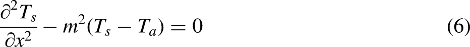
Combined convection-radiation coefficient

The heat is transferred from the rod to the external environment by a combination of radiation and convection. From a practical standpoint, the value of primary interest is the combined-mode heat transfer coefficient ${\overline{h}}^{*}$ , characterizing the fin parameter m. However, for a better understanding of the physical phenomena, the combined-mode heat transfer coefficient must be subdivided into its radiant and convective part, as follows

$${\overline{h}}^{*}={\overline{h}}_c+{\overline{h}}_r$$

(17)where ${\overline{h}}_c$ is the average convective heat transfer coefficient and ${\overline{h}}_r$ is the average radiant heat transfer coefficient given by the relationship

$$h_r=\sigma \epsilon F(T+T_a)(T^2+T_a^2)$$

(18)In the above equation, $\epsilon$ represents the surface emissivity, $F$ is the view factor, $T_a$ is the ambient temperature, while $\sigma$ is the Stefan-Boltzmann constant . ⁹ Thermal radiation is energy emitted by matter that is at a nonzero temperature. Regardless of the form of matter, the emission may be attributed to changes in the electron configurations of the constituent atoms or molecules at its surface. In this case, the fin emits energy toward other surfaces in the room because of the temperature gap between fin surface and walls. Since the fin surface is painted black and surrounded by walls, $\epsilon$ and F are equal to unity.

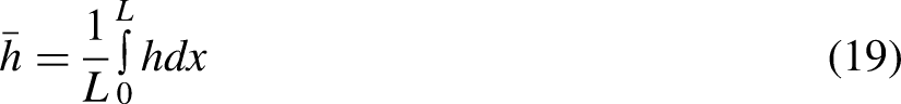
The average values of convective and radiant heat transfer coefficients are calculated on the fin length by

$$\overline{h}={\displaystyle \frac{1}{L}\underset{0}{\overset{L}{\int }}hdx}$$

(19)Free convection heat transfer from heated horizontal cylinders immersed in an extensive, quiescent fluid has been widely studied for over 50 years . ¹⁰ Even if discrepancies in all of the data still exist due to various factors, Churchill and Chu ¹¹ obtain the following expression for the average Nusselt number on horizontal cylinders for the laminar regime

$$N{u}_D=0,36+0,518{\left({\displaystyle \frac{R{a}_D}{{[1+{(0,559/Pr)}^{9/16}]}^{16/9}}}\right)}^{1/4}$$

(20)This correlation matches well with experimental data for all Prandtl numbers in the range of ${10}^{-6}<R{a}_D<{10}^9$ and is still widely used in free convection calculations. Nevertheless, other correlations are also available in literature for laminar free convection above horizontal cylinders (Morgan, Gaddar, Fand, Bansal and Chandna ¹⁰ ). It could be very interesting and instructive for students to compare the values of $h_c$ obtained using different correlations, experimenting by themselves to learn the importance of choosing the best formula to fit experimental data, and evaluating the associated uncertainty.

Results and discussion

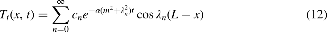
Experimental measurements of the axial temperature profile were carried out for four different voltages (9 V, 12 V, 14 V and 16 V). A higher voltage corresponds to a higher base temperature. Results are displayed in Fig. 2, where dotted lines represent the analytical solution and the points are the experimental temperatures at different t (120 s, 600 s, 1 200 s, 1 800 s, 2 700 s and 3 600 s).

Figure 2.

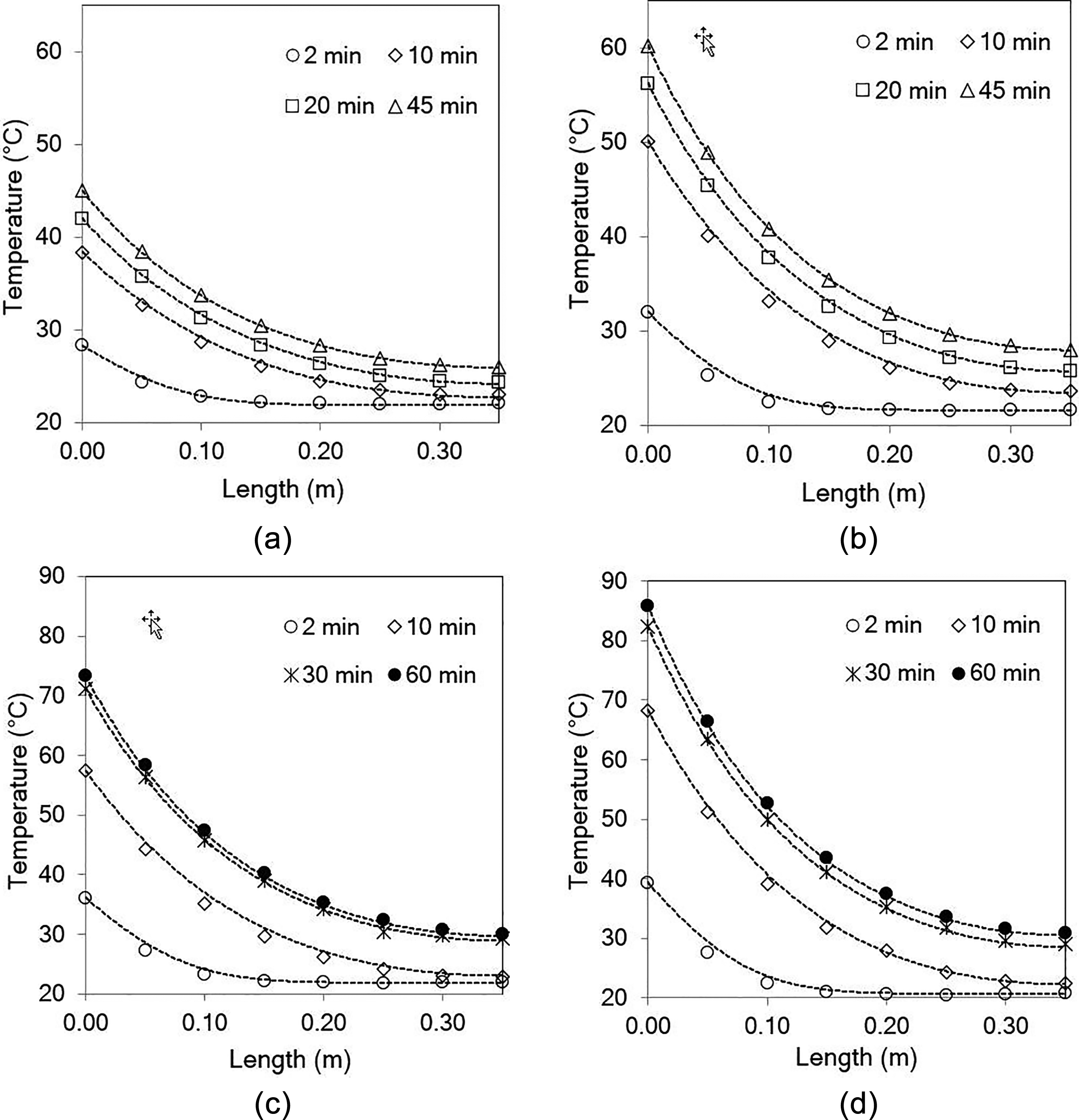
(a to d) Surface temperature: measured data (points) and analytical solutions (dotted lines) along the fin at different t and voltages: (a) $9.0V;R^2>0.991$ ; (b) $12.0V;R^2>0.985$ ; (c) $14.0V;R^2>0.989$ ; (d) $16.0V;R^2>0.988$ .

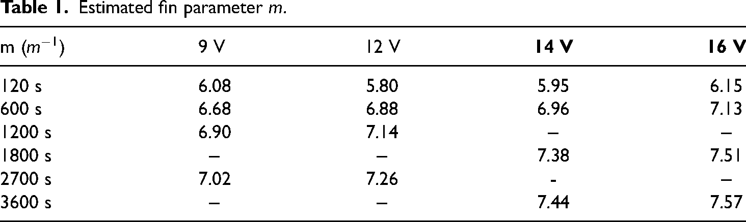
First of all, we calculated the average combined-mode heat transfer coefficients ${\overline{h}}^{*}$ using experimental temperatures. Then, we evaluated the fin parameter $m=\sqrt{{\overline{h}}^{*}P/k{A}_c}$ , for each set of experimental data, as reported in Table 1. Analytical solutions in Figure 2(a) to d were obtained using Equation (16) and the corresponding fin parameter. We approximated this infinite series by the sum of its first five terms. The addition of more terms to the sum does not significantly improve the approximation. The corresponding error was estimated calculating the coefficient of determination $R^2$ for each function. All values are based on two sums of squares: Sum of Squares Total (SST) and Sum of Squares Error (SSE). SST measures how far the experimental data are from the mean, and SSE measures how far the experimental data are from the model's predicted values. The difference between SST and SSE is the improvement in prediction from the model, compared to the mean model. Dividing that difference by SST gives $R^2$ . It has the useful property that its scale is intuitive. It ranges from zero to one. Zero indicates that the proposed model does not fit the experimental data. One indicates perfect prediction.

Table 1.

Estimated fin parameter m.

m $(m^{-1})$	9 V	12 V	14 V	16 V
120 s	6.08	5.80	5.95	6.15
600 s	6.68	6.88	6.96	7.13
1200 s	6.90	7.14	−	−
1800 s	−	−	7.38	7.51
2700 s	7.02	7.26	-	−
3600 s	−	−	7.44	7.57

As can be seen, the model fits the experiments very well, with a coefficient of determination $R^2$ that usually exceeds 0.985, even at low values of t. The fin parameters reported in Table 1 are similar to one other and fall in the expected range, increasing slightly with time and base temperature.

The value of primary interest is the combined-mode (radiation and convection) heat flux from the fin to the surroundings, which could be easily expressed as:

$$q=h^{*}(T-T_a)$$

(21)where $(T-T_a)$ represents the temperature difference between the surface temperature and the ambient air. In order to simplify the heat flux calculation, we consider that $T_a\cong T_{sur}$ . Moreover, the laboratory was large enough to ensure that walls, ceiling, and floor did not influence experimental results since surface resistances are considered negligible. Lastly, all air-physical properties were evaluated at the film temperature $T_f=(T+T_a)/2$ . The experimental values (Equation 21), as well as the predicted model values are presented in Figure 3. In general, the predictions of heat flux are well supported by the experimental values. However, the model tends to overestimate the total heat flux, especially at lower values of t, due perhaps to high uncertainty in the emissivity on the fin surface. Moreover, even if Eq. (20) is applicable for all Ra and Pr, the convection coefficient does not approach zero as Ra approaches zero, which is the case when t is small.

Figure 3.

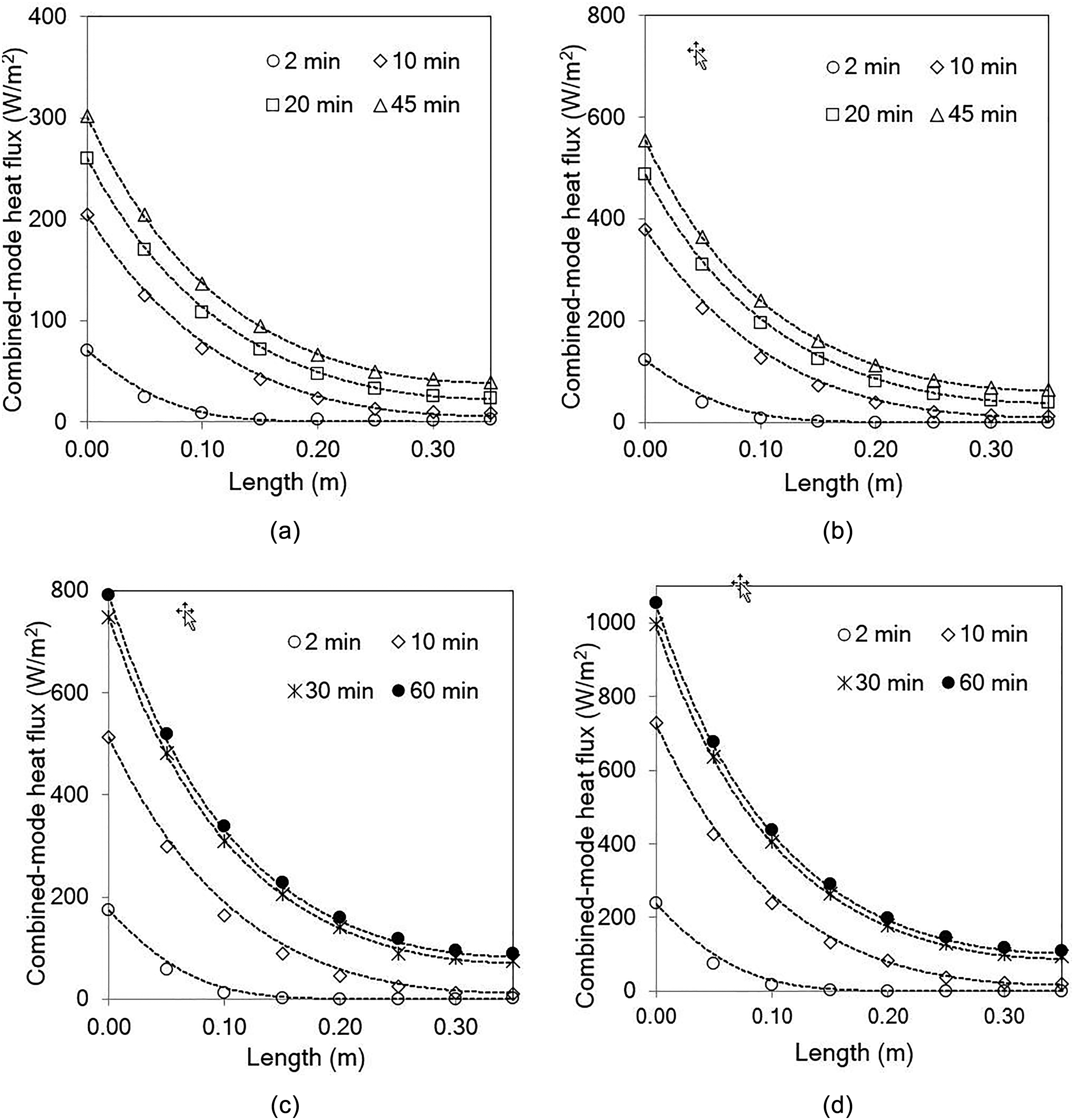
(a to d) Combined-mode heat flux: measured data (points) and analytical solutions (dotted lines) along the fin at different t and voltages: (a) $9.0V;R^2>0.991$ ; (b) $12.0V;R^2>0.985$ ; (c) $14.0V;R^2>0.989$ ; (d) $16.0V;R^2>0.988$ .

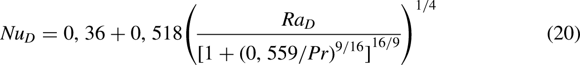
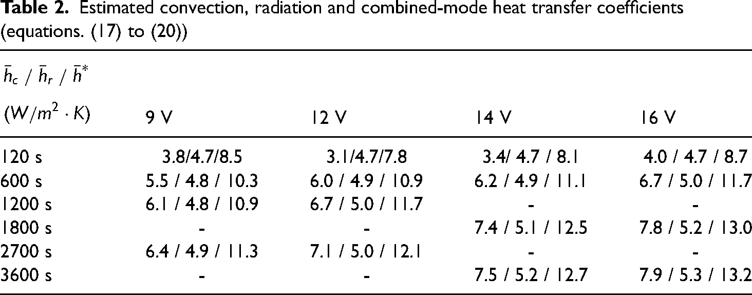
Convection, radiation and combined-mode coefficients calculated with experimental data using Equations. (17) to (20) are presented in Table 2. The convection coefficient increases rapidly with time and voltage, varying from 3.8 to 7.9 $W/m^2\cdot K$ , according to typical values present in literature, ¹⁰ while the radiation coefficient tends to be constant, close to 5.0 $W/m^2\cdot K$ .

Table 2.

Estimated convection, radiation and combined-mode heat transfer coefficients (equations. (17) to (20))

$\begin{array}{rl}& {\overline{h}}_c/{\overline{h}}_r/{\overline{h}}^{*}\\ & (W/m^2\cdot K)\end{array}$	9 V	12 V	14 V	16 V
120 s	3.8/4.7/8.5	3.1/4.7/7.8	3.4/ 4.7 / 8.1	4.0 / 4.7 / 8.7
600 s	5.5 / 4.8 / 10.3	6.0 / 4.9 / 10.9	6.2 / 4.9 / 11.1	6.7 / 5.0 / 11.7
1200 s	6.1 / 4.8 / 10.9	6.7 / 5.0 / 11.7	-	-
1800 s	-	-	7.4 / 5.1 / 12.5	7.8 / 5.2 / 13.0
2700 s	6.4 / 4.9 / 11.3	7.1 / 5.0 / 12.1	-	-
3600 s	-	-	7.5 / 5.2 / 12.7	7.9 / 5.3 / 13.2

The reason for carrying out the experiment at four different voltages is to show that this analysis is repeatable and well designed. A model could also be used to investigate the influence of some parameters, such as fin conductivity, geometric fin shape or the surrounding fluid properties, in order to extend the analysis and the understanding of basic heat transfer principles of extended surfaces. Finally, this simple experiment allows the confirmation of a complex theoretical description and could motivate students to develop advanced mathematical skills.

Example of extended surfaces laboratory application in undergraduate courses

Since the lab is the main part of the course, it should be emphasized through pre- and post-lab elements (Figure 4) in order to improve student conceptual understanding of extended surfaces as well as scientific reasoning .^{12, 13} In the pre-lab part, students receive the lab handout which gives detailed instructions on experimental procedure. Students work in small groups (3-4 students), organizing and sharing tasks. During this time, students could review all the theoretical subjects required to perform the lab (extended surface mathematical description, transient energy balance, free convection, and radiation heat transfer coefficient correlations, etc.), ask questions on lab objectives, and prepare Excel worksheets to facilitate the data collection. Even if the procedure is the same for all students, results, analysis, and interpretation may vary from one group to another.

Figure 4.

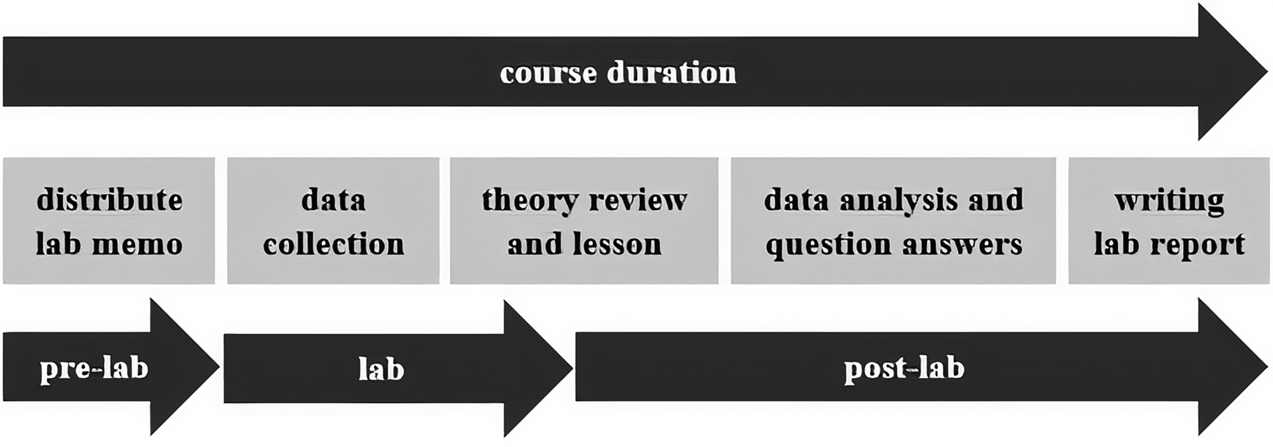
Lab structure.

Later, in the lab, students collect data together. Detailed instructions include how to turn on the electrical and the heating blocks, set the experimental voltages (9 V and then 16V, if time permits), read temperatures along the fin for different values of t using a chronometer. Moreover, students could measure fin dimensions $(d,L)$ and take the ambient temperature $T_a$ . Since the procedure provides many downtimes, students could start the analysis of collected data, discuss solution approaches, find appropriate correlations and equations to describe the transient conduction along the fin. Once all data have been collected, students finalize in the post-lab part the analysis of experimental data, develop the theoretical model, compare the results, and write the laboratory report. Analysis is the most important part of the entire lab (Figure 5). In fact, students have the possibility to verify firsthand that the analytical solution fits all experimental data very well and reproduces the temperature profile as well as the total heat flux.

Figure 5.

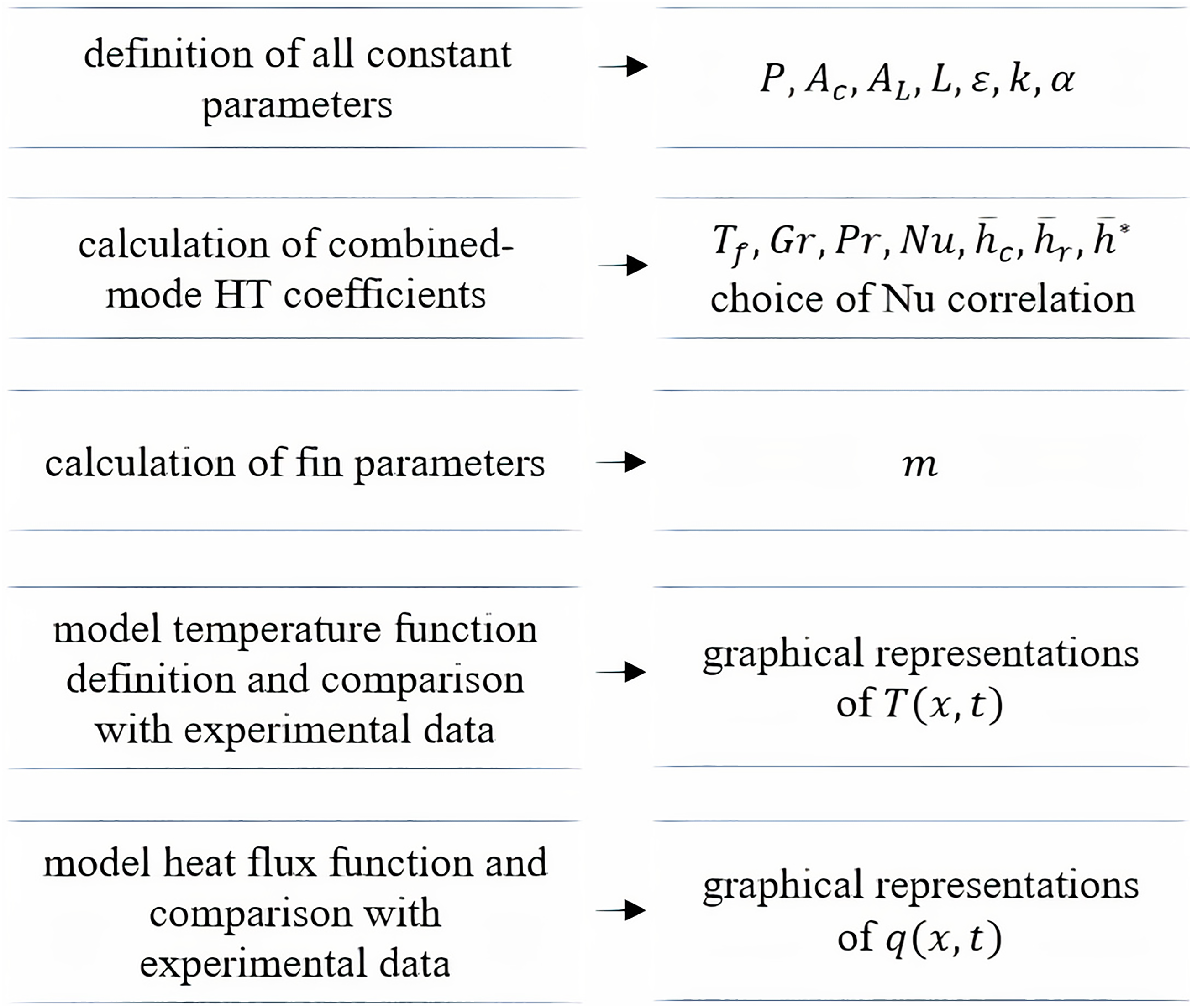
Analysis steps of experimental data.

Moreover, the combined-mode (free-convection and radiation) approach describes appropriately the heat transfer mechanism. Lastly, a comparison between different free-convection Nusselt correlations could allow the students to face the uncertainty of this calculation and make them reflect on the importance of the choice of the best correlation for their system.

Conclusion

The experimental fin device used in this paper led to the creation of an interesting experiment for undergraduate engineering students, which allowed them to develop a better understanding of transient, one-dimensional heat transfer with convection and radiation. The proposed analytical solution fits all experimental data very well and reproduces the temperature profile as well as the total heat flux with a coefficient of determination higher than 0.985. The combined-mode approach made it possible to evaluate the relative predominance of convection with respect to radiation, even if the radiation coefficient seems to be overestimated at lower values of t. The strong agreement between the measured results and the analytical solution, as well as the repeatability of the experiments demonstrates that it might be successfully used to propose to students a variety of interesting case studies over extended surfaces heat transfer. The model could also be used to investigate and compare the influence of some parameters, such as fin conductivity, geometric fin shape or the surrounding fluid properties.