
Abstract
The total poverty gap provides a straightforward information to policymakers as it measures the amount of income needed to get poor people out of poverty. Monitoring the change in total poverty gap is useful to examine poverty dynamics, however such a measure would be more informative if it were linked to other poverty indicators in a unified analysis framework. This paper suggests a decomposition that links the change in total poverty gap to those in poverty incidence, poverty depth, population size and composition. The decomposition is used to analyze the change in total poverty gap in Italy between 2010 and 2020. The total poverty gap decreased in the period considered and the change in poverty incidence was the main driver of such a reduction.
1. Introduction
The total poverty gap is one of the most widely used indicators of poverty as it quantifies the amount of income needed to get poor people out of poverty (Ziliak 2008). This straightforward information is often accompanied by the complementary information provided by other poverty indicators, such as the headcount ratio or the average income shortfall. Monitoring the changes in these indicators is crucial to provide policymakers with information on how poverty has changed after that some initiatives to counter the phenomenon have been taken. When looking at the changes in the various poverty indicators separately, one can know how poverty has changed from different viewpoints; however, the effects of such changes cannot be directly linked. For example, a 10% reduction in the headcount ratio says that the incidence of poverty in the population has decreased by that percentage, however we do not know the extent to which the total poverty gap has changed for such a poverty-reducing effect. This suggests that measuring the changes in poverty indicators would be more informative if these changes were analyzed in a unified framework. This article proposes a decomposition separating the change in total poverty gap into components linked to the changes in four factors: the poverty incidence, the average income shortfall, the population size and composition. While a change in total poverty gap is clearly related to those in poverty incidence, average income shortfall and population size, the link between a change in total poverty gap and that in population composition may be less evident. However, when the subpopulations within a population have different poverty levels, a change in the relative distribution of people among the subpopulations can have an impact on the total poverty gap. For example, if immigrants tend to be poorer than natives, as in most European immigrant-receiving countries (Bask 2005; Berti et al. 2014; Busetta 2016; De Bustillo and Anton 2011; Haisken-DeNew and Sinning 2010), the changes in the proportions of immigrants and natives in the population can have an effect on the total poverty gap.
Technically speaking, the decomposition of the change in total poverty gap is obtained by using the logarithmic mean Divisia index technique, the use of which is widely spread in studies on changes in energy efficiency (Ang and Choi 1997; Ang et al. 1998) as it is flexible and easy to interpret. Each component quantifies the variation in total poverty gap that would occur for the change observed in a single factor while the remaining factors are held constant over time. A further advantage of such a decomposition method is that the change in total poverty gap in a population can be examined by disaggregating the population into subpopulations and by measuring the effects of changes in poverty incidence and average income shortfall within each subpopulation.
The decomposition is used to analyze the change in total poverty gap for Italian families from 2010 to 2020. Italy has long-lasting economic disparities between northern and southern regions (Brandolini 2021; Fanti et al. 2023), resulting in territorial differences in terms of poverty incidence and depth (Benedetti and Crescenzi 2023; Ciommi et al. 2021). Such differences can be examined when using the decomposition as it can separate the effects of the changes in poverty within different subpopulations. In Italy, the main sources of poverty statistics are the Italian National Institute of Statistics (henceforth, Istat) and the Bank of Italy. Istat (2023) provides poverty statistics based on its own Survey on Income and Living Conditions. The Bank of Italy collects data useful for measuring poverty through the Survey on Household Income and Wealth (hereafter, SHIW). The data used in this study are from the SHIW historical archive, which includes the data collected in all surveys conducted by the Bank of Italy. Results show that the total poverty gap decreased over the 2010 to 2020 period and that a reduction in poverty incidence, especially in Southern Italy, had a major role in reducing the total poverty gap. The changes in population size and composition had poverty-increasing effects on the total poverty gap, however their magnitude was not enough to counterbalance the poverty-reducing impacts of the other components of the change in total poverty gap.
The article is organized as follows: Section 2 briefly reviews the literature on the decomposition of changes in poverty indicators and explains the rationale of the study; Section 3 describes the decomposition of the change in total poverty gap; Section 4 discusses the implications of a change in the poverty line when decomposing the change in total poverty gap; Section 5 shows the results of the decomposition applied to the change in total poverty gap calculated for Italian families between 2010 and 2020; Section 6 concludes.
2. Literature Review and Rationale of the Study
The decomposition of changes in poverty has been addressed by a number of studies in the literature on poverty measurement. A portion of the literature focused on decomposing the change in the whole income distribution to assess the contributions of different income sources in changing the entire distribution or a part of it (e.g., the bottom of the income distribution; Daly and Valletta 2006; Kyzyma et al. 2022; Larrimore 2014; Peichl et al. 2012). This distributional decomposition approach is generally applicable because it is not linked to a specific index or a class of indices (Kyzyma et al. 2022). Another part of the literature focused on the development of decomposition techniques useful for decomposing the change in a single poverty index or in each index belonging to a given class of indices. Khan and Azhar (2003) broke down the change in the headcount ratio by separating the contributions of changes in poverty incidence within different subpopulations from that of the change in population size. Datt and Ravallion (1992) proposed a decomposition, valid for a class of poverty indices, which separates an income-growth component from an income-redistribution component. A drawback of the Datt and Ravallion proposal is that the decomposition is not exact as a residual term is included. Kakwani (2000) suggested an alternative version of the Datt and Ravallion decomposition where there is no residual term. Within this field of research, Aristondo et al. (2023) proposed a decomposition which separates the effect of changes in the poverty line from that of changes in the income distribution. Feng et al. (2023) suggested a four-term decomposition of the change in the Foster-Greer-Thorbecke poverty index (Foster et al. 1984) which measures the effects of changes in the poverty line and income distribution. Mussard and Pi Alperin (2011) and Mussini (2013) proposed multi-dimensional decompositions of the change in the Sen-Shorrocks-Thon poverty index (Sen 1976; Shorrocks 1995; Thon 1979), linking the decomposition of the poverty change to the decomposition by subpopulation and income source, typically used for income inequality indices (De Battisti and Porro 2023; Ogwang 2016; Pasquazzi and Zenga 2018). Andreoli et al. (2021) suggested a decomposition of the poverty change for a new class of poverty indices; in addition, they obtained a spatial decomposition of each component of the poverty change to measure the neighborhood effect in poverty dynamics.
The above-mentioned studies, irrespective of which poverty measure is being considered, have the common purpose of quantifying the contributions of different factors to the change in poverty, providing further insights for the analysis of poverty change. A decomposition of the change in total poverty gap is based on the same rationale, which can be explained in detail by defining the poverty indicator firstly.
Consider a population of individuals in year
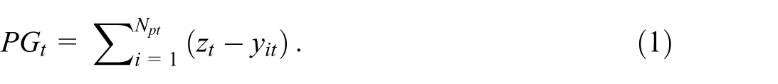
The total poverty gap in Equation (1) is a popular indicator of poverty as it measures how much income is needed to bring the incomes of poor individuals up to the poverty line. In other words, the total poverty gap indicates the amount of income which should be transferred to poor people for eliminating poverty. In spite of its straightforward interpretation, the total poverty gap has some drawbacks, such as the fact that it is not scale invariant (Kyzyma 2020). A further issue may arise when making comparisons over time, as a simple numerical example can explain. Table 1 shows the income distribution for ten income receivers in year
Example of Drivers of the Change in Total Poverty Gap.
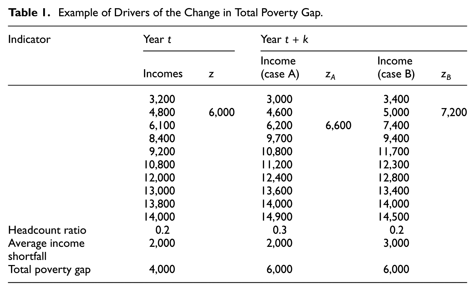
This example shows that a change in total poverty gap can be the result of changes in different factors, which cannot be assessed just by looking at the change in total poverty gap. To separate the contributions of different factors to the change in total poverty gap, an appropriate statistical tool is needed. Such a tool may be a decomposition that breaks down the change in total poverty gap into various components, as shown in the next section.
3. Decomposing the Change in Total Poverty Gap
Suppose that the population in year
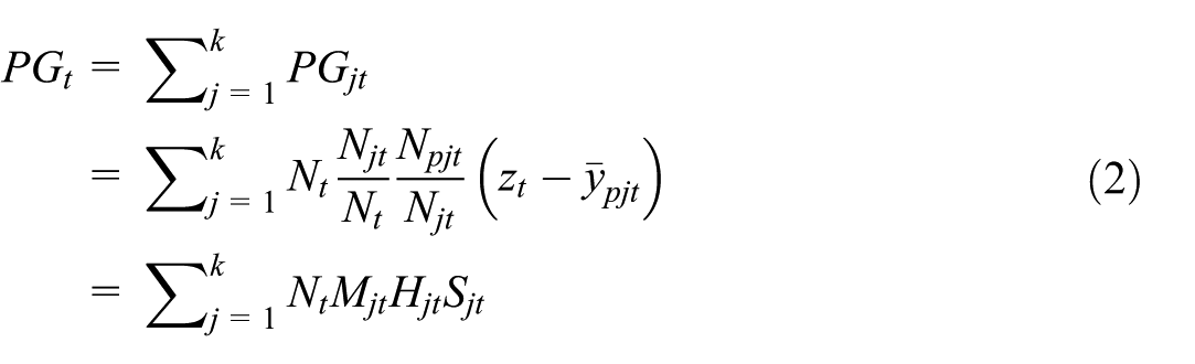
where
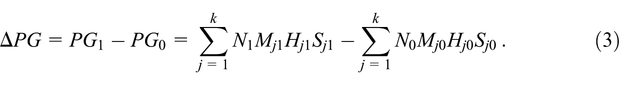
From Equation (2), the change in total poverty gap from year 0 to year 1 is
A necessary first step to split
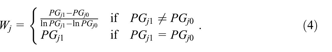
The logarithmic mean
Now, using
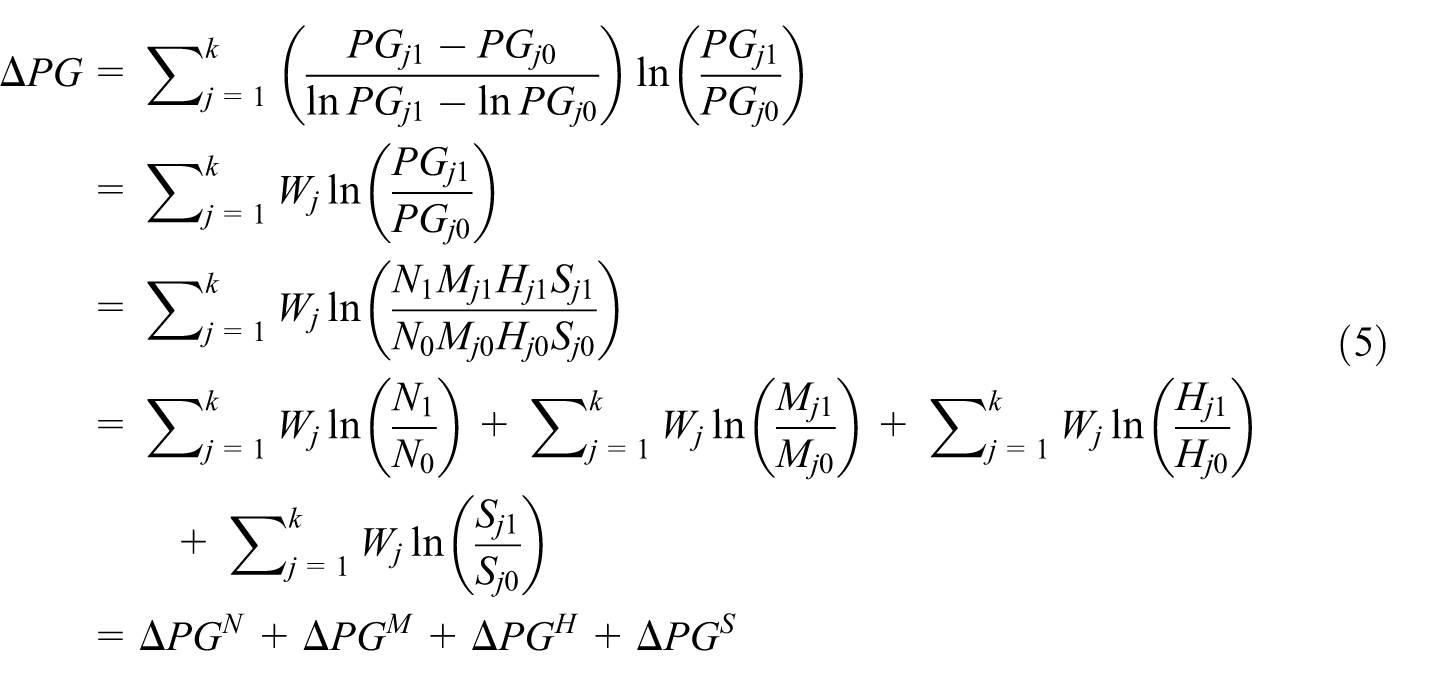
In Equation (5), the change in total poverty gap is broken down into four components.
The above decomposition has the advantage of linking the change in total poverty gap to the changes in population size and composition, poverty incidence, and poverty depth. This provides additional information to policymakers as the changes in such indicators are examined in a unified analysis framework rather than separately. For instance, if the population size grew while holding other things constant, the decomposition would show that the increase in total poverty gap is fully captured by the population-size component whereas the other components equal zero.
A further remark, from a practical standpoint, concerns the way in which the population is divided into subpopulations. Although the population partition is obtained by using a criterion which depends on the context under examination and the research scopes, a general recommendation is checking whether the total poverty gap within each subpopulation is equal to zero in year 0 or 1, which means that a subpopulation has no one below the poverty line in a certain year. As the decomposition in Equation (5) includes logarithmic terms, the presence of zero values would be problematic. While a subpopulation with no one below the poverty line is highly unlikely to be observed when the change in total poverty gap is measured at a national or regional level, a subpopulation of non-poor individuals might be observed at a disaggregated level of territorial analysis (e.g., at a neighborhood level). Also, a subpopulation with few poor individuals in year 0 or 1 should be carefully considered as it may give small values for the headcount ratio or the average income shortfall and therefore large relative changes in these indicators. However, such a situation is not as problematic as the zero-value issue above because each subpopulation
4. Separating the Poverty Line Effect
The change in total poverty gap in Equation (3) is measured by considering a poverty line related to the living standards in year 1,
The rationale underlying the above-mentioned decompositions can be applied to the decomposition of the change in total poverty gap described in section 3 because two out of four components, specifically the poverty-incidence and income-shortfall components, depend on how the poverty line varies between years 0 and 1. For each of these two components, the effect of the shift in the poverty line
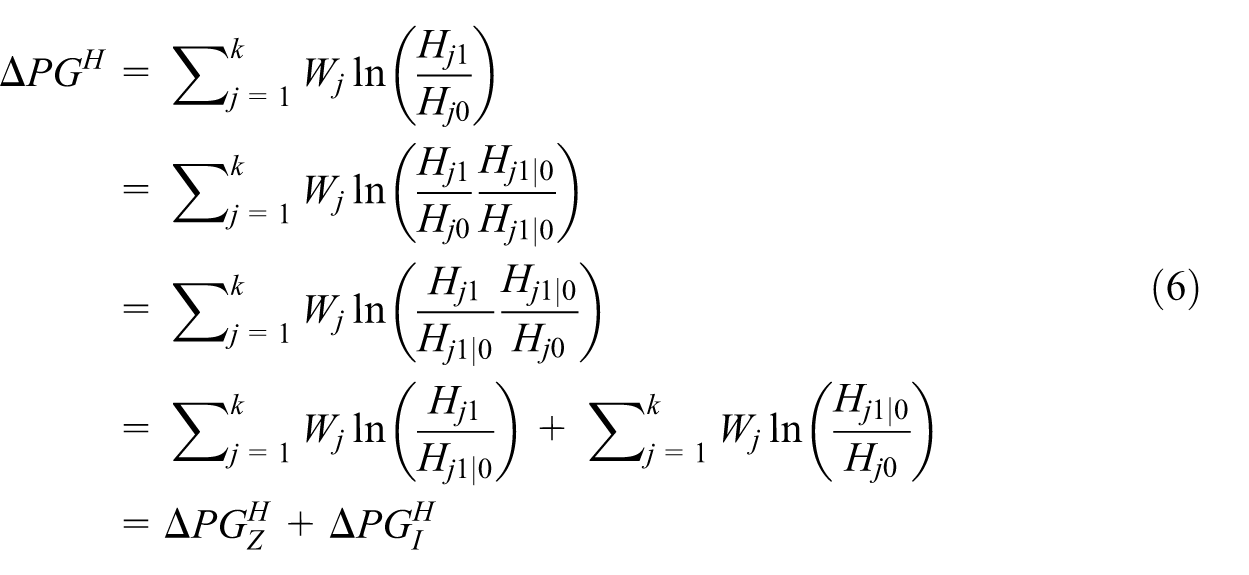
The other component,
The income-shortfall component in Equation (5) can be broken down by using the same approach above. Let

5. An Analysis of the Change in Total Poverty Gap in Italy
The decomposition is used to analyze the change in total poverty gap for Italian families from 2010 to 2020. Data are from the SHIW, conducted every two years by the Bank of Italy. The 2022 SHIW is the latest survey available and collected data referring to 2020. Such data are also included in the SHIW historical archive collecting information gathered in the surveys from 1977 to 2020 (Bank of Italy 2023). From this archive, we looked at the data on net disposable incomes, consumption expenditures, and other socio-demographic characteristics of Italian families in 2010 and 2020. 6,239 families were interviewed in 2020, while those interviewed in 2010 were 7,951. The SHIW historical archive includes sampling weights for comparisons over time, which were used in the analysis. The 2010 incomes and consumption expenditures were adjusted for inflation to be compared to those in 2020.
The decomposition of the change in total poverty gap in Equation (5) is obtained by dividing the population into three subpopulations by the macro-region of residence in Italy: North, Center, and South (with islands). This population partition is motivated by the long-lasting economic inequalities between northern and southern regions that characterize the country. Such a phenomenon, known as the “Italian North-South divide” (Fanti et al. 2023), has been investigated in several studies. Di Caro (2017) analyzed the income disparities between Italian regions by using administrative tax data in 2014, finding that income inequality was higher in Southern Italy than in North-Central Italy. Benedetti and Crescenzi (2023) estimated the proportion of families at-risk-of-poverty in every Italian region by using the 2018 EU-SILC data, showing that the proportions of families at-risk-of-poverty in southern regions were higher than those in northern regions.
Since family is the unit of observation in the analysis and the needs of a family change by the number and ages of members, a relative poverty line varying by family type is needed to establish whether a family is poor. To this purpose, firstly a poverty line has been computed for a single-person family; such a poverty line has been then multiplied by the coefficients of the modified OECD equivalence scale to find the poverty thresholds for other family types (e.g., a couple of adults, a couple of adults with a minor, …). The modified OECD equivalence scale assigns a value of 1 for the first adult, a value of 0.5 for each additional adult (aged 15 or over) in the family and a value of 0.3 for each child (aged 14 or under; Hagenaars et al. 1994). Table 2 shows the equivalence coefficients for some family types.
The Modified OECD Equivalence Scale.
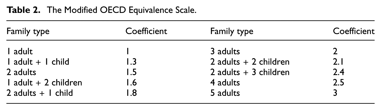
The relative poverty line for a single-person family in a certain year is set equal to the per capita consumption expenditure in that year. Such a way of setting the relative poverty line is similar to that used by Istat (2023), with the difference that Istat considers a two-person family as reference family type. This choice is motivated by the fact that Istat uses the Carbonaro equivalence scale, which sets a two-person family as reference family type, to adjust the poverty threshold on the basis of the family composition. The 2020 poverty line for the reference family type (single-person family) is equal to 9,207 € while the 2010 poverty line equals 11,015 €.
Figure 1 shows the headcount ratio in the three macro-regions calculated for 2010, where the disparities between the South and the Center-North are evident. These results confirm that Italy is characterized by territorial differences in poverty at the beginning of the period considered.
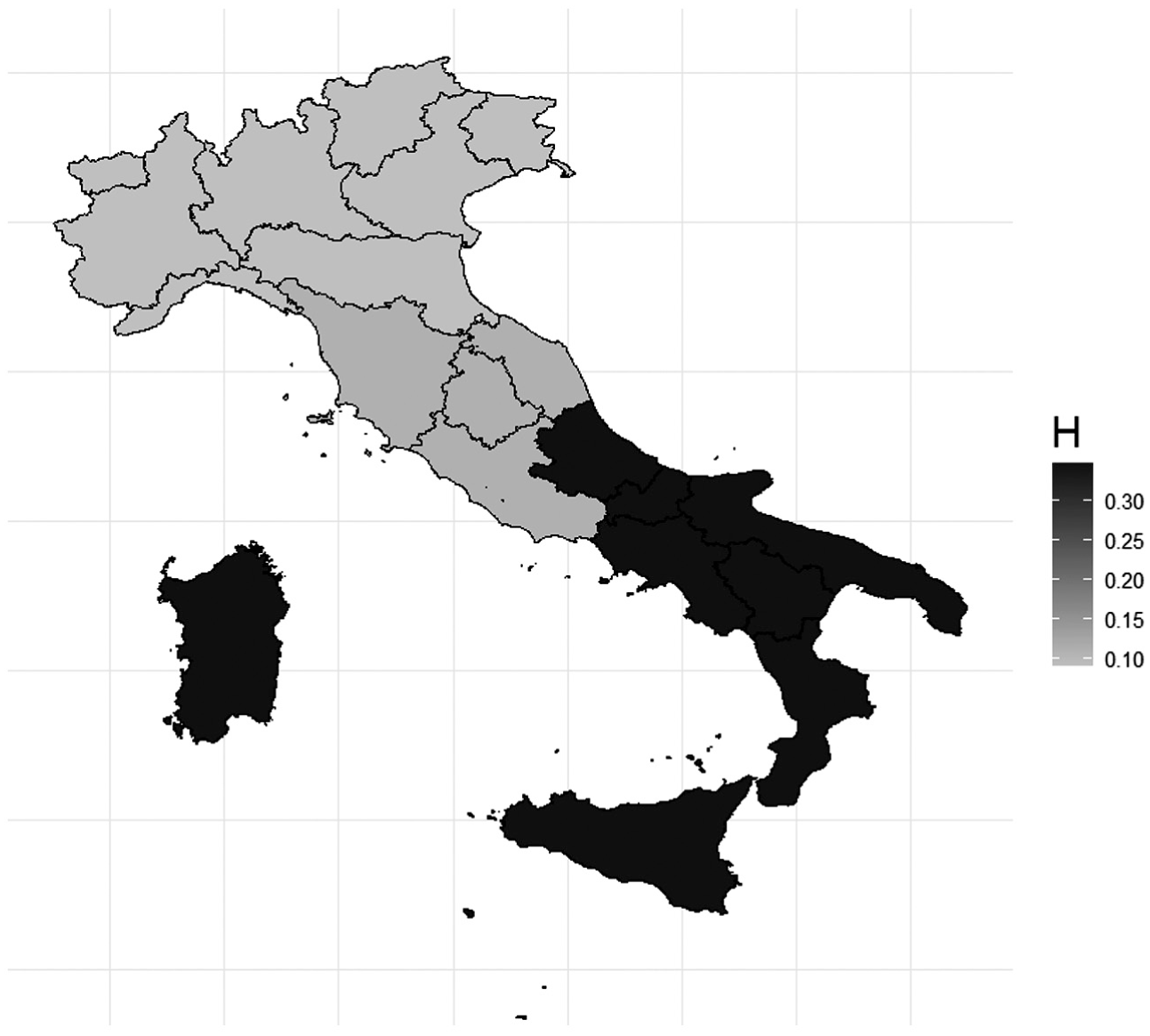
Headcount ratio in Italy in 2010 by macro-region.
Table 3 shows the headcount ratio, the average income shortfall and the Gini index for incomes of poor families in 2020 for each macro-region; in addition, the percentage changes in the poverty indicators compared to their values in 2010 are reported. Even though the inequality among poor families is not included in the decomposition of the total poverty gap, such an indicator has been calculated to complement the descriptive statistics on poverty in Italy in the period under consideration. Poverty incidence decreased in each area, with the Center and the South showing the largest reductions in relative terms. The average income shortfall decreased in the North and especially in the South (−24.13%) but increased in the Center (6.25%). The inequality among poor families increased in the North, decreased in the South and remained substantially stable in the Center between 2010 and 2020.
Headcount Ratio, Average Income Shortfall, and Gini Index in 2020 by Macro-Region.
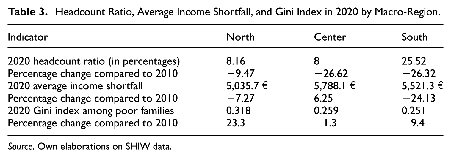
Source. Own elaborations on SHIW data.
The total poverty gap in 2010 is 27,327.4 million € while the change in total poverty gap between 2010 and 2020 is −8,299.9 million €, indicating that the amount of money needed to get poor families out of poverty decreased by almost a third over a decade. Now the decomposition can tell us which role was played by each factor in obtaining that change in total poverty gap. The four components of the change in total poverty gap are shown in Figure 2.
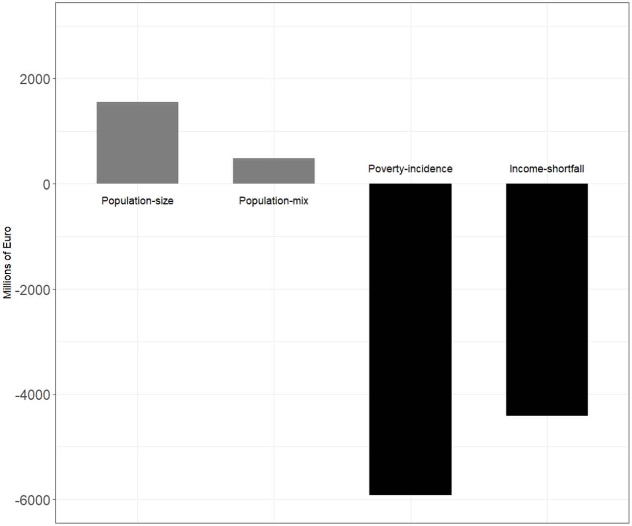
Components of the change in total poverty gap in Italy, 2010 to 2020.
The population-size component is positive, suggesting that the change in population size would have increased the total poverty gap between 2010 and 2020, other things being equal. In other words, 1,558.6 million € is the increase in total poverty gap that we would observe for effect of the increase in population if the other factors (the population-mix, subpopulation poverty incidences, and average income shortfalls) were unchanged from 2010 to 2020. The population-mix component is positive (480.5 million €) but smaller than the population-size component. Such an increase in the total poverty gap is linked to changes in the relative distribution of families among the three areas (North, Center, and South). More specifically, the increase in the proportion of families living in Southern Italy plays a major role in the population-mix component. The poverty-incidence component is negative and the largest one, in absolute terms, as the changes in subpopulation poverty incidences imply a decrease of 5,924.2 million € in the total poverty gap. This can be seen as the amount of savings to get families out of poverty in 2020, compared to 2010, for effect of the decreases in subpopulation headcount ratios. The most poverty-reducing effect comes from the reduction in poverty incidence occurred in the South. The income-shortfall component is negative, leading to a reduction of 4,414.9 million € in the total poverty gap. This measures the effect of a decrease in the average gap separating the income of a poor family from the relative poverty line.
The effects of the changes in the poverty line and family incomes on the poverty-incidence and income-shortfall components are shown in Figure 3. When considering the decomposition of
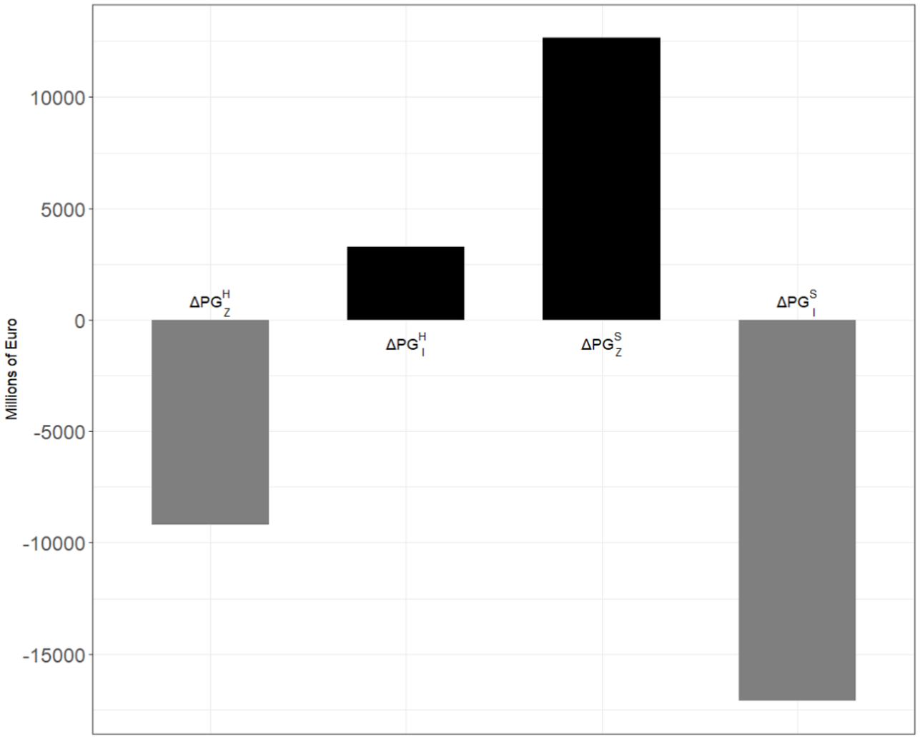
Decomposition of the poverty-incidence and income-shortfall components of the change in total poverty gap in Italy, 2010 to 2020.
To sum up, the decomposition shows that the changes in poverty incidence were the main driver of the decrease in total poverty gap between 2010 and 2020, overcoming also the poverty-reducing impact of the decreases in average income shortfall in Northern and Southern Italy. The variations in population size and composition, with their poverty-increasing effects, had a secondary role in changing the total poverty gap. From a policy point of view, the above results point out that a strategy focusing on the reduction of poverty incidence in southern regions could be well suited for achieving an appreciable reduction in the total poverty gap.
6. Conclusions
This article has shown that a given change in total poverty gap may result from alternative combinations of changes in poverty incidence, poverty depth, population size and composition. To overcome this issue, a four-term decomposition linking the change in total poverty gap to those in the four factors above has been obtained by using the logarithmic mean Divisia index decomposition technique (Ang and Choi 1997). The advantage of using such a decomposition is two-fold. First, policymakers can get new insights on the determinants of the change in total poverty gap, as a small change can be the result of different components that almost offset each other whereas a large change can be the outcome of different contributions which reinforce each other. Second, as the decomposition builds on the logarithmic mean Divisia index analysis, the computation of the various components is simple and the interpretation of such components is straightforward. Thus, the decomposition can be seen as a practical and informative statistical tool for examining the changes in total poverty gap. Even though such a decomposition can separate the effects of various drivers of the change in total poverty gap, the change in income inequality among the poor is not taken into consideration and this may be seen as a weakness of the decomposition.
The analysis of the change in total poverty gap in Italy between 2010 and 2020 has pointed out three main findings. The total poverty gap decreased by 8,299.9 million €, equal to 30.4% of the total poverty gap in 2010. The reduction in poverty incidence was the main driver of the change in total poverty gap, especially in Southern Italy where poverty incidence was higher than those in the Center and the North. The changes in population size and composition had poverty-increasing impacts on the total poverty gap, which partially offset the poverty-reducing effects of the other components.
A natural direction for future research is the application of the decomposition to other datasets, for instance the EU-SILC data, extending the study to other countries. Future research may also include the comparison of the results obtained by using alternative poverty lines. A poverty line based on consumption expenditures has been chosen for the analysis of the poverty change in Italy because such a choice is in line with the method used by Istat to set a relative poverty line. However, there are alternative ways of setting the poverty line, like fixing the poverty threshold equal to a certain percentage of the median equivalized income.
Footnotes
Acknowledgements
We would like to thank an Associate Editor and three anonymous reviewers for their helpful comments on an earlier version of this manuscript.
Funding
The authors received no financial support for the research, authorship, and/or publication of this article.
Received: August 11, 2024
Accepted: November 26, 2025