Estimation of Poverty Measures for Small Areas Under a Two-fold Nested Error Linear Regression Model: Comparison of Two Methods

Abstract

Demand for reliable statistics at a local area (small area) level has greatly increased in recent years. Traditional area-specific estimators based on probability samples are not adequate because of small sample size or even zero sample size in a local area. As a result, methods based on models linking the areas are widely used. World Bank focused on estimating poverty measures, in particular poverty incidence and poverty gap called FGT measures, using a simulated census method, called ELL, based on a one-fold nested error model for a suitable transformation of the welfare variable. Modified ELL methods leading to significant gain in efficiency over ELL also have been proposed under the one-fold model. An advantage of ELL and modified ELL methods is that distributional assumptions on the random effects in the model are not needed. In this article, we extend ELL and modified ELL to two-fold nested error models to estimate poverty indicators for areas (say a state) and subareas (say counties within a state). Our simulation results indicate that the modified ELL estimators lead to large efficiency gains over ELL at the area level and subarea level. Further, modified ELL method retaining both area and subarea estimated effects in the model (called MELL2) performs significantly better in terms of mean squared error (MSE) for sampled subareas than the modified ELL retaining only estimated area effect in the model (called MELLI).

AMS Subject Classification: 62D05, 62G09

1. Introduction

Data collected from probability samples can provide reliable estimates of parameters of interest for domains (subpopulations) with large enough sample sizes to permit direct, domain-specific estimators of desired precision. We call such domains as large areas. On the other hand, sample sizes can be very small or even zero for local areas (called small areas) and direct estimators are not adequate or feasible. Demand for reliable statistics at the level of small areas has increased greatly and it is necessary to use model-based methods that can yield reliable estimates for small areas by integrating information across areas through linking models. Rao and Molina^[13] provide a comprehensive account of model-based small area estimation of means, totals, and more complex parameters like poverty measures.

In this article, we focus on the estimation of FGT poverty measures, proposed by Foster et al.^[6] Poverty incidence, gap and severity belong to the family of FGT measures. World Bank widely used a method proposed by Elbers et al.^[5], called the ELL method, to provide FGT poverty measures for specified local areas in many developing countries. The ELL method involves the following steps: (a) Simulate multiple censuses of the welfare variable of interest based on an assumed model relating the welfare variable to auxiliary variables obtained from a recent census; (b) Calculate the FGT measure for specified local areas from each simulated census and then take the average over the censuses as the ELL estimator; (c) Variance of the simulated census estimators is taken as the estimator of mean squared error (MSE) of the ELL estimator. An advantage of the ELL method is that it is free of parametric distributional assumptions and computationally simple. However, Molina and RaO^[11] showed that the ELL method can lead to large MSE compared to an optimal method, called the Empirical Best (EB) method, assuming a one-fold nested error linear regression model with normally distributed random effects. Diallo and Rao^[4] developed a modification to ELL method that leads to substantial reduction in MSE and compares favorably to the normality-based EB method. As in the ELL method, the modified ELL method is free of parametric distributional assumptions. The proposed ELL, modified ELL and EB methods are based on a one-fold nested error linear regression model relating a suitable function of the welfare variable to the census variables and a random area effect. Sample survey data observing the welfare variable and the census variables, based on two-stage cluster sampling, are used to fit the one-fold model. In the traditional ELL method, random cluster effects are included in the model and simulated censuses are generated. From a simulated census, a desired poverty measure is calculated for any desired small area. Note that it is not necessary to specify the areas in advance because area effects are not included in the ELL one-fold model. Hossain et al.^[9] used a two-stage sample of districts and household within districts to estimate a food insecurity measure at the district level in Bangladesh. In this case, clusters are areas. In this article, we focus on two-fold random effect models involving area and subarea random effects. For example, an area could refer to a state and a subarea to a county within a state. Marhuenda et al.^[10] studied EB estimation of FGT poverty measures under the two-fold model, assuming that the random effects in the model are normally distributed, as in the case of the onefold model studied by Molina and Rao^[13]. In their application to Spanish survey data, areas are provinces and subareas are comarcas, and it is of interest to obtain estimates of poverty measures at the domain as well as subdomain level.

Section 2 sets the stage by briefly describing the ELL, modified ELL and EB methods for estimating poverty indicators for areas under a one-fold nested error regression model. Section 3 introduces the two-fold model and the associated FGT poverty measures for domains and subdomains. Section 4 extends the ELL and modified ELL methods to two-fold models with no distributional

assumptions on the random effects in the model, as in the case of the one-fold model. Section 5 presents some results of a simulation study on the performance of ELL and modified ELL estimators. Finally, some remarks on the estimation of MSE of the estimators are given in Section 6.

2. One-fold Nested Error Model

In this section, we introduce the ELL method and its modification (MELL), based on a one-fold nested error linear regression model relating a log transformation of a welfare variable of interest $E$ to known census variables $x$ for the finite population of interest. In the ELL method, a twostage cluster sample $\left\{\left(E_{dj},x_{dj}^T\right),d=1,\dots ,D;j=1,\dots ,n_d\right\}$ is used in conjunction with known population records/census variables $\left\{x_{dj},d=1,\dots ,D_p;j=1,\dots ,N_d\right\}$ , where $\left(D_p,D\right)$ denote the number of clusters in the population and the sample, and $\left(N_d,n_d\right)$ denote the number of population units and sample units in cluster $d$ . An intercept term is included in the covariate vector $x_{dj}$ . To reduce skewness in the welfare variable, a suitable transformation $y_{dj}=T\left(E_{dj}\right)$ is used, where $T($ . is one-to-one. In the ELL method, $y_{dj}=\text{log}\left(E_{dj}\right)$ is used. Typically, clusters are nested in the areas of interest. For simplicity, we assume here that clusters are the same as the areas.

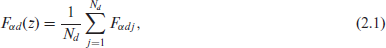
The FGT poverty indicator for area $d$ is given by

$$F_{\alpha d}\left(z\right)=\frac{1}{N_d}{\displaystyle \sum }_{j=1}^{N_d}{F}_{\alpha dj},$$

(2.1)

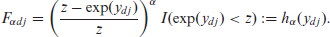
where

$$F_{\alpha dj}={\left(\frac{z-E_{dj}}{z}\right)}^{\alpha }I\left(E_{dj}<z\right).$$

(2.2)

In (2.2), $z$ is the known poverty line and $I\left(E_{dj}<z\right)$ is the indicator variable taking the value 1 when $E_{dj}$ is smaller than $z$ and 0 otherwise. Poverty incidence, poverty gap and poverty severity correspond to $\alpha =0,\alpha =1$ , and $\alpha =2$ , respectively. We use a one-to-one transformation $y_{dj}=$ $\text{log}\left(E_{dj}\right)$ of the welfare variable $E_{dj}$ . Often, a positive constant $c$ is added to $E_{dj}$ to ensure $E_{dj}+$ $c>0$ . Here we assume $E_{dj}>0$ for all the population units. We can express $F_{\alpha dj}$ in terms of the transformed variable $y_{dj}$ as

$$F_{\alpha dj}={\left(\frac{z-\text{exp}\left(y_{dj}\right)}{z}\right)}^{\alpha }I\left(\text{exp}\left(y_{dj}\right)<z\right):=h_{\alpha }\left(y_{dj}\right).$$

We focus here on the additive FGT poverty measures, ${\sum }_j{h}_{\alpha }\left(y_{dj}\right)$ , but the ELL method and its modifications are applicable to general measures of the form $h\left(y_{d1},\dots ,y_{d{N}_d}\right)$ .

2.1. ELL Method

We assume a one-fold nested error linear regression model relating $y_{dj}$ to $x_{dj}$ :

$$y_{dj}=x_{dj}^T\beta +u_d+e_{dj};d=1,\dots ,D_p,j=1,\dots ,N_d$$

(2.3)

where $u_d$ and $e_{dj}$ denote random area effect and residual error and independently distributed with means zero and variances ${\sigma }_u^2$ and ${\sigma }_e^2$ respectively. Parametric distributions on the two random effects are not assumed. Sampling is assumed to be non-informative in the sense that the population model holds for the sample data:

$$y_{dj}=x_{dj}^T\beta +u_d+e_{dj};d=1,\dots ,D,j=1,\dots ,n_d$$

(2.4)

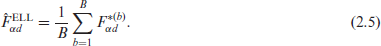
where we denote the first $n_d$ units as the sample in area $d$ , without loss of generality. The following steps are used in the ELL method: (a) Calculate the sample residuals $r_{dj}=y_{dj}-x_{dj}^T\hat{\beta }$ , where $\hat{\beta }$ is the ordinary least square (OLS) estimator of the regression coefficient $\beta$ in the sample model (2.4) with estimated covariance matrix ${\hat{V}}_{\beta }$ ; (b) The random area effect $u_d$ is estimated as ${\hat{u}}_d=n_d^{-1}{\sum }_j{r}_{dj}$ ; (c) Unit level residual $e_{dj}$ is estimated as ${\hat{e}}_{dj}=r_{dj}-{\hat{u}}_d$ . Two referees noted that the above estimators are equivalent to estimators obtained from an analysis of covariance model treating $u_d$ as fixed effect and imposing the condition ${\sum }_d{n}_d{u}_d=0$ ; (d) Draw $B$ sets of bootstrap values $\left\{\left({\hat{\beta }}^{\text{*}\left(b\right)},u_d^{\text{*}\left(b\right)},e_{dj}^{\text{*}\left(b\right)}\right),d=1,\dots ,D;j=1,\dots ,N_d\right\},b=1,\dots ,B$ from $N\left(\hat{\beta },{\hat{V}}_{\beta }\right)$ , the empirical distribution of ${\hat{u}}_d\left(d=1,\dots ,D\right)$ , and the empirical distribution of ${\hat{e}}_{dj}\left(d=1,\dots ,D;j=1,\dots ,N_d\right)$ , respectively; (e) Construct $B$ sets of simulated census values $y_{dj}^{\text{*}\left(b\right)}$ as follows: $\left\{y_{dj}^{\text{*}\left(b\right)}=x_{dj}^T{\hat{\beta }}^{\text{*}\left(b\right)}+\right.$ $\left.u_d^{\text{*}\left(b\right)}+e_{dj}^{\text{*}\left(b\right)},d=1,\dots ,D;j=1,\dots ,N_d\right\},b=1,\dots ,B$ , using the census values of the covariates $x_{dj}$ ; (f) Calculate simulated population FGT measures $F_{\alpha d}^{\text{*}\left(b\right)}=N_d^{-1}{\sum }_{j=1}^{N_d}{F}_{\alpha dj}^{\text{*}\left(b\right)},b=1,\dots ,B$ , where $F_{\alpha dj}^{\text{*}\left(b\right)}=h_{\alpha }\left(y_{dj}^{\text{*}\left(b\right)}\right)$ ; (g) Calculate the ELL estimator of $F_{\alpha d}$ by taking average of $F_{\alpha d}^{\text{*}\left(b\right)}$ over $b$ :

$${\hat{F}}_{\alpha d}^{\text{ELL}}=\frac{1}{B}{\displaystyle \sum }_{b=1}^B{F}_{\alpha d}^{\text{*}\left(b\right)}.$$

(2.5)

The ELL method is also applicable to non-sampled areas $d$ following steps 4-7 above.

2.2. Modified ELL Method

The modified ELL method, proposed by Diallo and Rao,^[4] retains the estimated area effects ${\hat{u}}_d$ for sampled area $d$ , unlike using $u_d^{\text{*}\left(b\right)}$ as in the ELL method. The simulated values $y_{dj}^{\text{*}\left(b\right)}$ are generated from $y_{dj}^{\text{*}\left(b\right)}=x_{dj}^T\hat{\beta }+{\hat{u}}_d+e_{dj}^{\text{*}\left(b\right)}$ and steps (f) and (g) above are implemented using the simulated values to calculate the modified ELL (MELL) estimator of $F_{\alpha d}$ , denoted as ${\hat{F}}_{\alpha d}^{\text{MELL}}$ . For non-sampled areas $d$ we use the ELL method by generating the simulated values $y_{dj}^{\text{*}\left(b\right)}$ from $y_{dj}^{\text{*}\left(b\right)}=x_{dj}^T\hat{\beta }+u_d^{\text{*}\left(b\right)}+e_{dj}^{\text{*}\left(b\right)}$ .

A simulation study with skew normal error $e_{dj}$ showed large gain in efficiency for MELL estimator over ELL estimator for sampled areas $d$ . For non-sampled areas $d$ , ELL and MELL are the same. Diallo^[3] studied the performance of MELL when the ELL estimator ${\hat{u}}_d$ is replaced by the EBLUP estimator of $u_d$ , using moment estimators of the variance components in the nested error model (2.4) which are distribution-free. The resulting MELL estimators of the FGT measures were not significantly more efficient than the MELL estimators based on the ELL estimators ${\hat{u}}_d$ . A plausible reason for this lack of improved efficiency is due to the fact that the EBLUP estimators of the $u_d$ are designed for optimal estimation of the area means of the transformed variables $y_{dj}$ and not for estimating FGT measures for the areas.

In the special case of area mean ${\overline{Y}}_d$ , its ELL estimator is approximately equal to the synthetic estimator ${\overline{X}}_d^T\hat{\beta }$ for all areas, as noted in Molina and Rao^[13]. On the other hand, MELL estimator of ${\stackrel{࿽}{Y}}_d$ for a sampled area $d$ is approximately equal to the sample regression estimator ${\overline{y}}_d+{\left({\overline{X}}_d-{\overline{x}}_d\right)}^T\hat{\beta }$ , where ${\overline{y}}_d$ and ${\overline{x}}_d$ are the sample means for area $d$ . For a non-sampled area, MELL estimator of ${\overline{Y}}_d$ reduces to the synthetic estimator.

Both ELL and MELL are applicable to more complex measures, such as the Gini coefficient and the Fuzzy Monetary Index (Neri et al.^[12]). Those measures are not additive non-linear functions of the welfare variable $E_{dj}$ , unlike the FGT measure. An advantage of those complex measures over the FGT measure is that the knowledge of the poverty line is not required. Further, note that both ELL and MELL do not require linking the sample file to the population register from where the auxiliary variables $x_{dj}$ are obtained.

2.3. EB Method

Molina and Rao^[13] studied empirical best (EB) estimation of FGT poverty measures, assuming normality of the area effects $u_d$ and the unit errors $e_{dj}$ . The best estimator of $h_{\alpha }\left(y_{dj}\right)$ for a non-sampled unit $j$ in area $d$ is obtained as the expectation with respect to the conditional distribution of $y_{dj}$ given the vector of sampled values in area $d$ . A closed form expression for the best estimator does not exist in general, but it can be approximated by simulating $y_{dj}^{\left(l\right)},l=1,\dots ,L$ from the conditional distribution. Molina and Rao^[13] showed that $y_{dj}^{\left(l\right)}$ can be generated from a univariate normal distribution. EB estimator is obtained by replacing the model parameters in the best estimator by suitable estimators.

A limitation of EB estimation is that it requires linking the sample to the population for identifying the non-sampled units in each area, unlike ELL estimation. If linking is not feasible, then we can obtain EB estimator of $h_{\alpha }\left(y_{dj}\right)$ for all the population units $j$ in area $d$ , leading to Census EB estimator (Guadarrama et al.^[8]). The Census EB estimator is less efficient than the EB estimator when linking is feasible, but the loss in efficiency is small when the area sampling fraction is small. Corral-Rodas et al.^[2] provide refinements and extensions to the EB method of Molina and Rao (MR). A referee noted that the poverty maps produced by the World Bank recently were based on the EB method rather than the ELL method.

Diallo and Rao^[4] studied EB estimation under the one-fold model (2.4) with skew normal (SN) errors $e_{dj}$ and normal area effects $v_d$ . Their simulation results showed that the normality-based EB of Molina and Rao^[11] can be inefficient due to inflation of MSE caused by substantial bias in the estimator. However, the EB estimator of Diallo and Rao^[4] is very complex, and they proposed a simplified EB method which performed quite well compared to the EB method under SN errors. The modified ELL method is less efficient than the tailor-made EB methods of Diallo and Rao^[4] under the model with SN errors. Note that distributional assumptions on $u_d$ and $e_{dj}$ are not needed for the ELL and modified ELL methods. Graf et al.^[7] developed EB estimators by modelling the welfare variable $E_{dj}$ directly using a Generalized Beta distribution of the Second Kind.

3. Two-fold Nested Error Model

As in Marhuenda et al.^[10], the finite population of interest consists of $D$ areas (domains) $d=$ $1,\dots ,D$ , and area $d$ is divided into $M_d$ subareas (subdomains) $j=1,\dots ,M_d$ . The subdomain $j$ within the domain $d$ contains $N_{dj}$ elements $k=1,\dots ,N_{dj}$ . The population data is denoted as $\left\{\left(E_{djk},x_{djk}^T\right),d=1,\dots ,D;j=1,\dots ,M_d;k=1,\dots ,N_{dj}\right\}$ , where $E_{djk}$ is the welfare variable of interest and $x_{djk}^T=\left(x_{1djk},\dots ,x_{pdjk}\right)$ is a $p$ -vector of known census variables. If an intercept term is needed, then we set $x_{1djk}=1$ for all the population units. To reduce skewness in the welfare variable, a suitable transformation $y_{djk}=T\left(E_{djk}\right)$ is used. For the FGT poverty measures, we make a $\text{log}$ transformation $y_{djk}=\text{log}\left(E_{djk}\right)$ , assuming $E_{djk}>0$ for all the population units, as in Section 2.

A two-fold nested error population model relating the transformed variable $y_{djk}$ to the census variables $x_{djk}$ is given by

$$y_{djk}=x_{djk}^T\beta +u_d+v_{dj}+e_{djk};d=1,\dots ,D,j=1,\dots ,M_d,k=1,\dots ,N_{dj},$$

(3.1)

where $\beta$ is a $p\times 1$ vector of unknown regression parameters, $u_d$ are the area effects, $v_{dj}$ are the cluster effects, and $e_{djk}$ are the residual errors. The three random errors $u_d,v_{dj}$ , and $e_{djk}$ are independent with $\text{E}\left(u_d\right)=\text{E}\left(v_{dj}\right)=\text{E}\left(e_{djk}\right)=0$ . Parametric distributions on the two random effects and the unit errors are not assumed.

We assume two-stage sampling in each area: a sample, $s_d$ , of $m_d\left(\le M_d\right)$ subareas is selected from area $d$ and if subarea $j$ is sampled then a subsample, $s_{dj}$ of $n_{dj}$ elements is selected from subarea $j$ . We further assume that the population model (3.1) also holds for the sample data $\left\{\left(y_{djk},x_{djk}\right),d=\right.$ $\left.1,\dots ,D;j=1,\dots ,m_d;k=1,\dots ,n_{dj}\right\}$ . Therefore, the model for the sample data is given by

$$y_{djk}=x_{djk}^T\beta +u_d+v_{dj}+e_{djk};d=1,\dots ,D,j=1,\dots ,m_d,k=1,\dots ,n_{dj}.$$

(3.2)

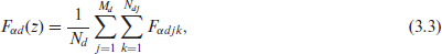
The FGT population measure for area $d$ is given by

$$F_{\alpha d}\left(z\right)=\frac{1}{N_d}{\displaystyle \sum }_{j=1}^{M_d}{\displaystyle \sum }_{k=1}^{N_{dj}}{F}_{\alpha djk},$$

(3.3)

where $N_d={\sum }_j{N}_{dj}$ and

$$F_{\alpha djk}={\left(\frac{z-E_{djk}}{z}\right)}^{\alpha }I\left(E_{djk}<z\right).$$

(3.4)

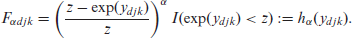
In (3.4), $z$ is the known poverty line and $I\left(E_{djk}<z\right)$ is the indicator variable taking the value 1 when $E_{djk}$ is smaller than $z$ and 0 otherwise. Also, the FGT measure for subarea $j$ within area $d$ is given by

$$F_{\alpha dj}\left(z\right)=\frac{1}{N_{dj}}{\displaystyle \sum }_{k=1}^{N_{dj}}{F}_{\alpha djk}.$$

(3.5)

4. Estimators of FGT Poverty Measures

In this section, we describe how to estimate FGT poverty measures (3.3) and (3.5) for areas and subareas, respectively. Suppose that there is a one-to-one transformation $y_{djk}=\text{log}\left(E_{djk}\right)$ of the welfare variables, assuming $E_{djk}>0$ for all the population units. Then we can express $F_{\alpha djk}$ given by (3.4) in terms of $y_{djk}$ :

$$F_{\alpha djk}={\left(\frac{z-\text{exp}\left(y_{djk}\right)}{z}\right)}^{\alpha }I\left(\text{exp}\left(y_{djk}\right)<z\right):=h_{\alpha }\left(y_{djk}\right).$$

4.1. ELL Method

In this section, we extend the ELL method under the one-fold nested error model to the two-fold nested error model (3.1) when the model has area level random effect term, unit level random effect term, and unit level error term. The proposed extension of the ELL method to two-fold models consists of drawing from the estimated area, subarea and unit level residuals to create a simulated census. The steps of the ELL method can be summarized as follows:

Estimate $\beta$ from the nested error model given by (3.2) and obtain unit level residuals ${\hat{r}}_{djk}=y_{djk}-x_{djk}^T\hat{\beta }$ where $\hat{\beta }$ denotes the OLS estimator of $\beta$ .

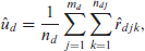
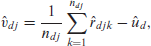
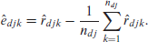
The area effect $u_d$ , the subarea effect $v_{dj}$ , and the unit level errors $e_{djk}$ are estimated as

$${\hat{u}}_d=\frac{1}{n_d}{\displaystyle \sum }_{j=1}^{m_d}{\displaystyle \sum }_{k=1}^{n_{dj}}{\hat{r}}_{djk},$$

$${\hat{v}}_{dj}=\frac{1}{n_{dj}}{\displaystyle \sum }_{k=1}^{n_{dj}}{\hat{r}}_{djk}-{\hat{u}}_d,$$

and

$${\hat{e}}_{djk}={\hat{r}}_{djk}-\frac{1}{n_{dj}}{\displaystyle \sum }_{k=1}^{n_{dj}}{\hat{r}}_{djk}.$$

Draw ${\hat{\beta }}^{\text{*}\left(b\right)},u_d^{\text{*}\left(b\right)},v_{dj}^{\text{*}\left(b\right)}$ , and $e_{djk}^{\text{*}\left(b\right)},b=1,\dots ,B$ from $N\left(\hat{\beta },{\hat{V}}_{\beta }\right)$ , the empirical distribution of ${\hat{u}}_d$ , the empirical distribution of ${\hat{v}}_{dj}$ , and the empirical distribution of ${\hat{e}}_{djk}$ , respectively. Also, ${\hat{V}}_{\beta }$ denotes the estimated covariance of $\hat{\beta }$ .

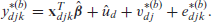
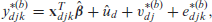
Construct $B$ simulated census values $\left\{y_{djk}^{\text{*}\left(b\right)};k=1,\dots ,N_{dj},j=1,\dots ,M_d,d=1,\dots ,D\right\}$ as follows: $y_{djk}^{\text{*}\left(b\right)}=x_{djk}^T{\hat{\beta }}^{\text{*}\left(b\right)}+u_d^{\text{*}\left(b\right)}+v_{dj}^{\text{*}\left(b\right)}+e_{djk}^{\text{*}\left(b\right)}$ , using the census values of the covariates.

Population measures $F_{\alpha d}^{\text{*}\left(b\right)}=\frac{1}{N_d}{\sum }_{j=1}^{M_d}{\sum }_{k=1}^{N_{dj}}{F}_{\alpha djk}^{\text{*}\left(b\right)}$ and $F_{\alpha dj}^{\text{*}\left(b\right)}=\frac{1}{N_{dj}}{\sum }_{k=1}^{N_{dj}}{F}_{\alpha djk}^{\text{*}\left(b\right)}$ are calculated from each simulated census $b$ , where $F_{\alpha djk}^{\text{*}\left(b\right)}=h_{\alpha }\left(y_{djk}^{\text{*}\left(b\right)}\right),b=1,\dots ,B$ .

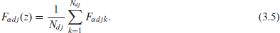
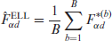
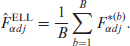
The ELL estimators of $F_{\alpha d}$ and $F_{\alpha dj}$ are calculated by averaging over the $B$ simulated measures as follows:

$${\hat{F}}_{\alpha d}^{\text{ELL}}=\frac{1}{B}{\displaystyle \sum }_{b=1}^B{F}_{\alpha d}^{\text{*}\left(b\right)}$$

and

$${\hat{F}}_{\alpha dj}^{\text{ELL}}=\frac{1}{B}{\displaystyle \sum }_{b=1}^B{F}_{\alpha dj}^{\text{*}\left(b\right)}.$$

The estimators ${\hat{u}}_d$ and ${\hat{v}}_{dj}$ are similar to those obtained under an analysis of covariance model treating $u_d$ and $v_{dj}$ as fixed and imposing side conditions on $u_d$ and $v_{dj}$ to ensure estimability, as done in the case of the one-fold model studied in section 2.1.

4.2. Modified ELL Methods

Method 1. This modification retains ${\hat{u}}_d$ in constructing the predictors $y_{djk}^{\text{*}\left(b\right)}$ , unlike the use of $u_d^{\text{*}\left(b\right)}$ in the ELL method. We have the following modified ELL method:

From the nested error model given by (3.2), estimate the fixed effects $\beta$ using OLS.

Estimate $u_d,v_{dj}$ , and $e_{djk}$ as in the traditional ELL method.

Draw $v_{dj}^{\text{*}\left(b\right)}$ and $e_{djk}^{\text{*}\left(b\right)},b=1,\dots ,B$ from the empirical distributions of ${\hat{v}}_{dj}$ and ${\hat{e}}_{djk}$ , respectively.

Construct $B$ simulated census values $\left\{y_{djk}^{\text{*}\left(b\right)};k=1,\dots ,N_{dj},j=1,\dots ,M_d,d=1,\dots ,D\right\}$ as follows:

$$y_{djk}^{\text{*}\left(b\right)}=x_{djk}^T\hat{\beta }+{\hat{u}}_d+v_{dj}^{\text{*}\left(b\right)}+e_{djk}^{\text{*}\left(b\right)}.$$

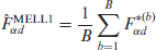
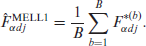
Then, the simulated population measures $F_{\alpha d}^{\text{*}\left(b\right)}$ and $F_{\alpha dj}^{\text{*}\left(b\right)}$ are calculated as in the traditional ELL method from each simulated census $b$ . The modified ELL estimators of $F_{\alpha d}$ and $F_{\alpha dj}$ , denoted by ${\hat{F}}_{\alpha d}^{\text{MELL}1}$ and ${\hat{F}}_{\alpha dj}^{\text{MELL}1}$ , respectively, are as follows:

$${\hat{F}}_{\alpha d}^{\text{MELL}1}=\frac{1}{B}{\displaystyle \sum }_{b=1}^B{F}_{\alpha d}^{\text{*}\left(b\right)}$$

and

$${\hat{F}}_{\alpha dj}^{\text{MELL}1}=\frac{1}{B}{\displaystyle \sum }_{b=1}^B{F}_{\alpha dj}^{\text{*}\left(b\right)}.$$

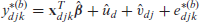
Method 2. This modification retains ${\hat{u}}_d$ and ${\hat{v}}_{dj}$ , for $j\in s_d$ , and uses $v_{dj}^{\text{*}\left(b\right)}$ for subarea $j$ not sampled from area $d$ in constructing the predictors $y_{djk}^{\text{*}\left(b\right)}$ . Then, the modification is as follows:

From the nested error model given by (3.2), estimate the fixed effects $\beta$ using OLS.

Estimate $u_d,v_{dj}$ , and $e_{djk}$ as in the traditional ELL method.

Draw $e_{djk}^{\text{*}\left(b\right)},b=1,\dots ,B$ from the empirical distribution of ${\hat{e}}_{djk}$ .

Construct $B$ simulated census values $y_{djk}^{\text{*}\left(b\right)}$ for the units in the sampled subareas as

$$y_{djk}^{\text{*}\left(b\right)}=x_{djk}^T\hat{\beta }+{\hat{u}}_d+{\hat{v}}_{dj}+e_{djk}^{\text{*}\left(b\right)}$$

and for subareas that are not sampled $y_{djk}^{\text{*}\left(b\right)}$ are generated from

$$y_{djk}^{\text{*}\left(b\right)}=x_{djk}^T\hat{\beta }+{\hat{u}}_d+v_{dj}^{\text{*}\left(b\right)}+e_{djk}^{\text{*}\left(b\right)},$$

where $v_{dj}^{\text{*}\left(b\right)},b=1,\dots ,B$ , are drawn from the empirical distribution ${\hat{v}}_{dj}$ .

Then, the simulated population measures $F_{\alpha d}^{\text{*}\left(b\right)}$ and $F_{\alpha dj}^{\text{*}\left(b\right)}$ are calculated as in the traditional ELL method from each simulated census $b$ , and the second modified ELL estimators of $F_{\alpha d}$ and $F_{\alpha dj}$ , denoted by ${\hat{F}}_{\alpha d}^{\text{MELL}2}$ and ${\hat{F}}_{\alpha dj}^{\text{MELL}2}$ , respectively, are as follows:

$${\hat{F}}_{\alpha d}^{\text{MELL}2}=\frac{1}{B}{\displaystyle \sum }_{b=1}^B{F}_{\alpha d}^{\text{*}\left(b\right)}$$

and

$${\hat{F}}_{\alpha dj}^{\text{MELL}2}=\frac{1}{B}{\displaystyle \sum }_{b=1}^B{F}_{\alpha dj}^{\text{*}\left(b\right)}.$$

In the special case of area mean ${\overline{Y}}_d$ , its ELL estimator is approximately equal to the synthetic estimator ${\overline{X}}_d^T\hat{\beta }$ , as noted in Marhuenda et al.^[10] On the other hand, both MELL1 and MELL2 estimators for a sampled area are approximately equal to the sample regression estimator ${\overline{y}}_d+\left({\overline{X}}_d-\right.$ ${\left.{\overline{x}}_d\right)}^T\hat{\beta }$ . For a non-sampled area, both reduce to the synthetic estimator.

Turning to a subarea mean ${\overline{Y}}_{dj}$ , MELL1 is approximately equal to ${\overline{X}}_{dj}^T\hat{\beta }+\left({\overline{y}}_d-{\overline{x}}_d^T\hat{\beta }\right)$ for all subareas within a sampled area. On the other hand, MELL2 is approximately equal to the subarea level sample regression estimator ${\overline{y}}_{dj}+{\left({\overline{X}}_{dj}-{\overline{x}}_{dj}\right)}^T\hat{\beta }$ for a sampled subarea. For a non-sampled subarea within a sampled area, MELL2 is equal to MELL1. For subareas within a non-sampled area, both MELL1 and MELL2 estimators are approximately equal to the synthetic estimator ${\overline{X}}_{dj}^T\hat{\beta }$ . On the other hand, ELL estimator for all subareas is approximately equal to the synthetic estimator ${\overline{X}}_{dj}^T\hat{\beta }$ .

4.3. EB Method

Marhuenda et al.^[10] studied EB estimation of FGT poverty measures for area and subareas under the two-fold nested error model (3.1), assuming the population model holds for the sample. This leads to the sample model (3.2). Unlike the ELL method, they assume normality of the area effects $u_d$ , subarea effects $v_{dj}$ and unit errors $e_{djk}$ . The model on the unit error $e_{djk}$ permits unequal variance ${\sigma }_e^2/w_{djk}$ with known heteroscedasticity weight $w_{djk}$ . Under the above set-up, they extended the EB method of Molina and Rao^[11] to derive EB estimators of FGT measures for areas and both sampled and non-sampled subareas within an area. This EB method is applicable only to additive measures like the FGT measure. They also conducted an extensive simulation study and compared the EB estimators for subareas under the two-fold model with those obtained under models with only subarea effects, when all subareas are sampled or not sampled. Here we consider the special case of $w_{djk}=1$ and denote the EB estimator of Marhuenda et al.^[10] as EB2.

5. Simulation Study

We conduced a simulation study to examine the performance of the two modified ELL methods under the two-fold nested error linear regression model (3.1). Marhuenda et al.^[10] conducted a simulation study on the performance of EB estimators of FGT measures for areas and subareas under a two-fold nested error model assuming $u_d,v_{dj}$ and $e_{djk}$ are normally distributed. We follow their simulation set-up but also considered a skew normal scenario with $\left(u_d,v_{dj}\right)$ normal (N) and $e_{djk}$ skew normal (SN). Marhuenda et al.^[10] made an extensive study for the two-fold model in the normal case, by fixing ${\sigma }_e$ and considering two marginal scenarios for $\left({\sigma }_u,{\sigma }_u\right)$ : (a) ${\sigma }_u$ fixed and ${\sigma }_v$ varied; (b) ${\sigma }_v$ fixed and ${\sigma }_u$ varied. The range of values considered included ${\sigma }_u=0$ corresponding to a model with subarea effects only, and ${\sigma }_v=0$ corresponding to a model with area effects only. Their results suggested that assuming the two-fold model when the correct model involves only area random effect or subarea random effect may not lead to significant loss in efficiency. We also included the case of $\left(u_d,v_{dj},e_{djk}\right)$ normal (N) studied by Marhuenda et al.^[10]

We set ${\sigma }_e=0.50$ as in Marhuenda et al.^[10], and consider two scenarios for setting the values of ${\sigma }_u$ and ${\sigma }_v$ : (a) Between area variation ${\sigma }_u=0.5$ is larger than the between subarea variation ${\sigma }_v=0.25$ ; (b) ${\sigma }_u=0.25$ is smaller than ${\sigma }_v=0.5$ . We also considered the case of smaller ${\sigma }_u$ and ${\sigma }_v$ to reflect more accurate covariates in the model: (c) ${\sigma }_u=0.1$ and ${\sigma }_v=0.2$ .

We generated $I=1,000$ populations each of size $N=20,000$ composed of $D=40$ areas each containing $M_d=10$ subareas each containing $N_{dj}=50$ units. As in Marhuenda et al.^[10], all the areas are sampled. We first generated the covariate vector $x_{djk}={\left(1,x_{1djk},x_{2djk}\right)}^{\text{'}}$ for each population unit, based on $x_{1djk}\sim \text{B}\left(1,p_{1dj}\right)$ and $x_{2djk}\sim \text{B}\left(1,p_{2dj}\right)$ with probabilities $p_{1dj}=0.2+$ $\frac{0.4d}{D}+\frac{0.4j}{M_d}$ and $p_{2dj}=0.2,j=1,\dots ,10,d=1,\dots ,40$ . The generated population covariate values are held fixed and used to generate the dependent variable $y_{djk}$ from the two-fold model using $\beta ={(3,0.03,-0.04)}^{\text{'}}$ and specified distributions for $u_d,v_{dj}$ , and $e_{djk}$ with mean zero and standard deviations ${\sigma }_u,{\sigma }_v$ and ${\sigma }_e$ , respectively. For the $\text{SN}$ case, we took $u_d\sim \text{N}\left(0,{\sigma }_u^2\right),v_{dj}\sim \text{N}\left(0,{\sigma }_v^2\right)$ and $e_{djk}\sim \text{SN}\left(\mu ,{\sigma }^2,\lambda \right)$ with $\mu$ and $\sigma$ chosen to make the mean and standard deviation of $e_{djk}$ equal to zero and ${\sigma }_e$ , and $\lambda ={\lambda }_e=3$ which leads to moderate skewness. As in Marhuenda et al.^[10], we set $E_{djk}=\text{exp}\left(y_{djk}\right)$ . The above process was repeated to generate $I=1000$ population values $\left\{y_{djk}^{\left(i\right)},i=1,\dots ,1000\right\}$ .

We calculated the FGT measures $F_{\alpha d}^{\left(i\right)}$ for each area and $F_{\alpha dj}^{\left(i\right)}$ for each subarea from each of the simulated populations $i=1,\dots ,1000$ . We focus on poverty incidence $\left(\alpha =0\right)$ and poverty gap $\left(\alpha =1\right)$ . Following Marhuenda et al.^[10], we took the poverty line as $z=0.6\text{med}\left(E_{djk}\right)$ for a population generated as above.

We considered two cases for generating a sample of units. In case 1, all subareas are sampled $\left(m_d=M_d=10\right)$ by selecting $n_{dj}=10$ units from each subarea by simple random sampling. In case 2, a simple random sample of $m_d=5$ subareas is selected from each area and then a simple random sample of $n_{dj}=20$ units is drawn from each sampled subarea. In both cases, the over all sample size within each area is equal to 100 and the number of bootstrap simulated censuses, $B$ , is taken as $B=50$ .

As in Marhuenda et al.^[10], we used a model-based set up by conditioning on the selected sample of units and extracting the corresponding sample data $\left(y_{djk}^{\left(i\right)},x_{djk}\right)$ from each simulated population $i$ . Using the sample data, we then obtained the desired estimates for areas and subareas from the assumed two-fold model. Denoting the estimators for areas and subareas for any given method by ${\hat{F}}_{\alpha d}$ and ${\hat{F}}_{\alpha dj}$ respectively, we computed empirical MSEs of the estimators for areas and subareas as

$$\text{MSE}\left({\hat{F}}_{\alpha d}\right)=I^{-1}{\displaystyle \sum }_{i=1}^I{\left({\hat{F}}_{\alpha d}^{\left(i\right)}-F_{\alpha d}^{\left(i\right)}\right)}^2,\text{ MSE}\left({\hat{F}}_{\alpha dj}\right)=I^{-1}{\displaystyle \sum }_{i=1}^I{\left({\hat{F}}_{\alpha dj}^{\left(i\right)}-F_{\alpha dj}^{\left(i\right)}\right)}^2,$$

where ${\hat{F}}_{\alpha d}^{\left(i\right)}$ and ${\hat{F}}_{\alpha dj}^{\left(i\right)}$ denote the estimators for the simulated population $i$ .

5.1. $e_{djk}$ Skew Normal

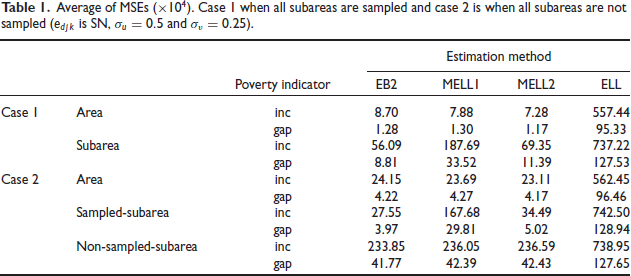
Table 1 reports results on average MSE for the areas, sampled subareas and non-sampled subareas for scenario 1: ${\sigma }_u=0.5$ and ${\sigma }_v=0.25$ . Table 1 shows that ELL leads to very large average MSE in all cases compared to the other methods. For areas, MELL2 and MELL1 are comparable and slightly better than EB2 in terms of average MSE. For subareas when all subareas are sampled (case 1), MELL2 leads to large reduction in average MSE over MELL1. This is to be expected because MELL1 does not use subarea specific method unlike MELL2. Also, EB2 seems to be somewhat better than MELL2 in terms of average MSE: 8.81 for EB2 vs. 11.39 for MELL2 in the case of poverty gap.

Table 1.

Average of MSEs $\left(\times {10}^4\right)$ . Case I when all subareas are sampled and case 2 is when all subareas are not sampled ( ${\text{e}}_{\text{djk}}$ is $\text{SN},{\sigma }_u=0.5$ and $\left.{\sigma }_v=0.25\right)$ .

			Estimation method
		Poverty indicator	EB2	MELLI	MELL2	ELL
Case I	Area	inc	8.70	7.88	7.28	557.44
		gap	1.28	1.30	1.17	95.33
	Subarea	inc	56.09	187.69	69.35	737.22
		gap	8.81	33.52	11.39	127.53
Case 2	Area	inc	24.15	23.69	23.11	562.45
		gap	4.22	4.27	4.17	96.46
	Sampled-subarea	inc	27.55	167.68	34.49	742.50
		gap	3.97	29.81	5.02	128.94
	Non-sampled-subarea	inc	233.85	236.05	236.59	738.95
		gap	41.77	42.39	42.43	127.65

Turning to case 2 where not all subareas are sampled, results for sampled subareas are similar those for case 1 where all subareas are sampled. Note that the average MSE is significantly decreased for sampled subareas because the sample size in those subareas is doubled relative to case 1. On the other hand, for areas the average MSE is significantly increased in case 2 compared to case 1 because the number of sampled subareas is reduced by half compared to case 1.

For nonsampled subareas (case 2), MELL1, MELL2 and EB2 are comparable in terms of average MSE. This is to be expected because for non-sampled subareas MELL1 and MELL2 are similar. Note that the average MSE is significantly increased for nonsampled subareas compared to corresponding values for sampled subareas. Box plots (not presented here) lead to conclusions like those arrived from the values of average MSE.

Table 2.

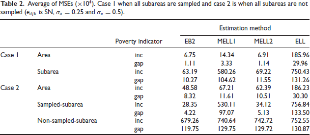
Average of MSEs $\left(\times {10}^4\right)$ . Case I when all subareas are sampled and case 2 is when all subareas are not sampled ( ${\text{e}}_{\text{djk}}$ is $\text{SN},{\sigma }_u=0.25$ and $\left.{\sigma }_v=0.5\right)$ .

			Estimation method
		Poverty indicator	EB2	MELLI	MELL2	ELL
Case I	Area	inc	6.75	14.34	6.91	185.96
		gap	1.11	3.33	1.14	29.96
	Subarea	inc	63.19	580.26	69.22	750.43
		gap	10.27	104.62	11.55	131.26
Case 2	Area	inc	48.58	67.21	62.39	186.23
		gap	8.32	11.61	10.51	30.30
	Sampled-subarea	inc	28.35	530.11	34.12	756.84
		gap	4.22	97.07	5.13	133.50
	Non-sampled-subarea	inc	679.26	740.64	742.72	752.55
		gap	119.75	129.75	129.72	130.87

Table 2 reports results on average MSE for scenario 2: ${\sigma }_u=0.25$ and ${\sigma }_v=0.5$ , corresponding to those in Table 1 for scenario 1. Comparing the two tables, conclusions for the case all subareas are sampled are similar for EB2 and MELL2, but average MSE for MELL1 has significantly increased. For the case not all subareas are sampled, average MSE values for EB2, MELL1 and MELL2 are substantially increased for areas, although conclusions are similar. For sampled subareas, EB2 and MELL2 gave similar average MSE values. For nonsampled subareas in case 2, MELL1, MELL2 and ELL are comparable in terms of average MSE while EB2 exhibits slightly smaller average MSE.

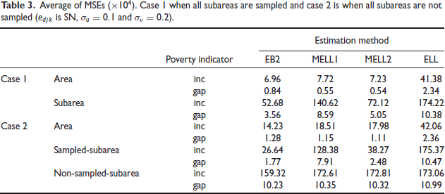
Results on average MSE for scenario 3 with ${\sigma }_u=0.1$ and ${\sigma }_v=0.2$ are reported in Table 3. For the case 1 with all subareas sampled, MELL1 and MELL2 are similar for areas in terms of average MSE, and slightly larger than the average MSE for EB2. ELL leads to a much larger average MSE for areas in both cases 1 and 2. Turning to subareas, MELL2 leads to large reduction in MSE relative to MELL1 and ELL, and slightly larger average MSE relative to EB2 in both cases 1 and 2. For the nonsampled subareas in case 2, average MSE is comparable across EB2, MELL1, MELL2 and ELL. Note that scenario 3 is favorable to ELL because the area and subarea effects are small.

Table 3.

Average of MSEs $\left(\times {10}^4\right)$ . Case I when all subareas are sampled and case 2 is when all subareas are not sampled ( ${\text{e}}_{\text{djk}}$ is $\text{SN},{\sigma }_u=0.I$ and ${\sigma }_v=0.2$ ).

			Estimation method
		Poverty indicator	EB2	MELLI	MELL2	ELL
Case I	Area	inc	6.96	7.72	7.23	41.38
		gap	0.84	0.55	0.54	2.34
	Subarea	inc	52.68	140.62	72.12	174.22
		gap	3.56	8.59	5.05	10.38
Case 2	Area	inc	14.23	18.51	17.98	42.06
		gap	1.28	1.15	1.11	2.36
	Sampled-subarea	inc	26.64	128.38	38.27	175.37
		gap	1.77	7.91	2.48	10.47
	Non-sampled-subarea	inc	159.32	172.61	172.81	173.06
		gap	10.23	10.35	10.32	10.99

5.2. $\left(u_d,v_{dj},{\text{e}}_{\text{djk}}\right)$ Normal

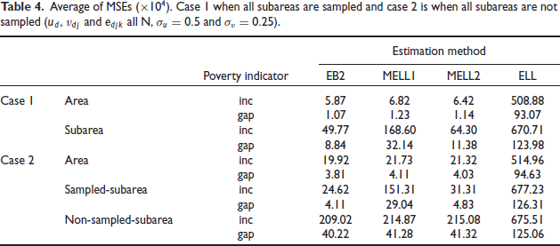
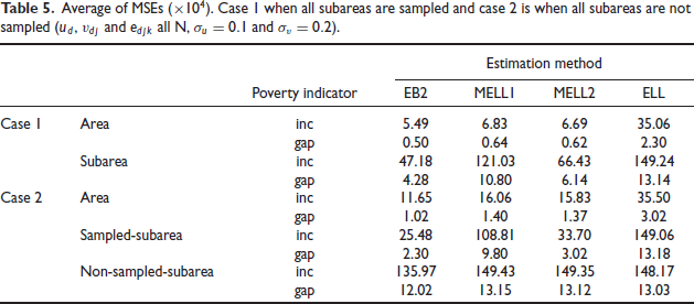
We also considered the case where $u_d,v_{dj}$ and $e_{djk}$ are normally distributed. Marhuenda et al.^[10] studied this case in the context of EB2. Table 4 gives the average MSE under scenario 1. Table 4 indicates that the results on MSE for areas, sampled subareas and non-sampled subareas are similar with the results in section 5.1 corresponding to skew normal. We also note that EB2 leads to substantial reduction in average MSE over MELL2 for subareas in case 1 where all subareas are sampled: 49.77 vs. 64.30 for incidence and 8.84 vs. 11.38 for gap. This is to be expected because EB2 is optimal under normality. Table 5 reports average MSE for the normal case under scenario 3. Results are similar to those in Table 4.

Table 4.

Average of MSEs $\left(\times {10}^4\right)$ . Case I when all subareas are sampled and case 2 is when all subareas are not sampled $\left(u_d,v_{dj}\right.$ and $e_{djk}$ all $\text{N},{\sigma }_u=0.5$ and $\left.{\sigma }_v=0.25\right)$ .

		Poverty indicator	Estimation method
			EB2	MELLI	MELL2	ELL
Case I	Area	inc	5.87	6.82	6.42	508.88
		gap	1.07	1.23	1.14	93.07
	Subarea	inc	49.77	168.60	64.30	670.71
		gap	8.84	32.14	11.38	123.98
Case 2	Area	inc	19.92	21.73	21.32	514.96
		gap	3.81	4.11	4.03	94.63
	Sampled-subarea	inc	24.62	151.31	31.31	677.23
		gap	4.11	29.04	4.83	126.31
	Non-sampled-subarea	inc	209.02	214.87	215.08	675.51
		gap	40.22	41.28	41.32	125.06

Table 5.

Average of MSEs $\left(\times {10}^4\right)$ . Case I when all subareas are sampled and case 2 is when all subareas are not sampled $\left(u_d,v_{dj}\right.$ and ${\text{e}}_{djk}$ all $\text{N},{\sigma }_u=0.I$ and $\left.{\sigma }_v=0.2\right)$ .

			Estimation method
		Poverty indicator	EB2	MELLI	MELL2	ELL
Case 1	Area	inc	5.49	6.83	6.69	35.06
		gap	0.50	0.64	0.62	2.30
	Subarea	inc	47.18	121.03	66.43	149.24
		gap	4.28	10.80	6.14	13.14
Case 2	Area	inc	11.65	16.06	15.83	35.50
		gap	1.02	1.40	1.37	3.02
	Sampled-subarea	inc	25.48	108.81	33.70	149.06
		gap	2.30	9.80	3.02	13.18
	Non-sampled-subarea	inc	135.97	149.43	149.35	148.17
		gap	12.02	13.15	13.12	13.03

6. MSE Estimation

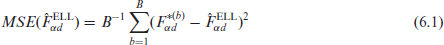
In the ELL method for the one-fold model, the variability of the simulated census measures is taken as the estimator of MSE of the ELL estimator. Similarly, under the two-fold model the corresponding MSE estimators of ELL for areas and subareas are given by

$$\text{MSE}\left({\hat{F}}_{\alpha d}^{\text{ELL}}\right)=B^{-1}{\displaystyle \sum }_{b=1}^B{\left(F_{\alpha d}^{\text{*}\left(b\right)}-{\hat{F}}_{\alpha d}^{\text{ELL}}\right)}^2$$

(6.1)

and

$$\text{MSE}\left({\hat{F}}_{\alpha dj}^{\text{ELL}}\right)=B^{-1}{\displaystyle \sum }_{b=1}^B{\left(F_{\alpha dj}^{\text{*}\left(b\right)}-{\hat{F}}_{\alpha dj}^{\text{ELL}}\right)}^2.$$

(6.2)

MSE estimators similar to (6.1) and (6.2) are applicable to MELL1 and MELL2, using simulated census measures. The proposed MSE estimators are simple, but they can lead to significant underestimation of the true MSE because the model parameters and the random effects in the model are not re-estimated in each replicate from the replicated sample data $\left(y_{djk}^{\text{*}\left(b\right)},x_{djk}\right)$ .

Marhuenda et al.^[10] proposed a proper parametric bootstrap MSE estimator for EB2 estimators, based on re-estimating model parameters and random effects in the two-fold model under normality. A similar procedure may be developed for ELL and MELL using a distribution free bootstrap, like the ELL method.

7. Concluding Remarks

We considered the estimation of FGT poverty measures under a two-fold nested error model. We developed extensions of the ELL method and the modified ELL method of Diallo and Rao^[4] to twofold models. The methods are free of parametric distributional assumptions on the random effects in the two-fold model. Our simulation results indicate that the proposed modified ELL methods lead to large efficiency gains over the ELL for both areas and subareas. Further, MELL2 leads to significant reduction in MSE over MELL1 for sampled subareas, and it is comparable to the EB2 method of Marhuenda et al.^[10] under normality assumption. Our simulation study is somewhat limited. It would be desirable to conduct a more extensive simulation study with different parameter combinations, as well as design-based simulations, as in Marhuenda et al.^[10] Bootstrap MSE estimation for MELL methods, along the lines of Marhuenda et al.^[10] but without normality assumption, needs a detailed investigation.

The EB2 method of Marhuenda et al.^[10] is applicable to additive functions like the FGT measures, and its extensions to more complex parameters remain to be investigated. On the other hand, as noted earlier, MELL2 is readily applicable to general parameters, not necessarily additive in the individual values like the FGT measures.