In this article, the estimators based on data from independent non-probability and probability samples are combined to estimate finite population parameters. Assuming that the values of the study variable are available in both samples, the integration of the non-probability and probability samples through a composite estimator of the population total is studied. The integration is done using a linear combination of the inverse probability weighted (IPW) estimator and a design-based estimator. By evaluating the variance of the former estimator, the randomness of the underlying non-probability sample is taken into account through the distribution of the estimated propensity scores. This approach is then compared with a variance estimator based on the asymptotic variance and with a bootstrap variance estimator. The proposed linear combination is not sensitive to the misspecification of the model for the propensity scores due to the incorporated estimator of the bias of the IPW estimator. The number of Lithuanian companies possessing websites is estimated in a simulation study. By combining the sample survey data and big voluntary sample data, the properties of the introduced estimators are demonstrated numerically.
Probability sampling methods are a generally accepted approach for surveying finite populations. Even for a relatively small probability sample from a finite population, valid inferences can be drawn using a known sampling design and models. Over the years, probabilistic sample-based methods have been well-developed for solving various finite population problems (Cochran 1977; Särndal et al. 1992; Tillé 2020; Wu and Thompson 2020).
However, with time passing, the situation is changing. Nowadays, probability surveys have significant drawbacks: their costs are relatively high, participation rates are decreasing, and the accuracy of estimates becomes lower. At the same time, the number of non-probability data sets is increasing. They consist of administrative data sources that record business events, data derived by sensors and machines when measuring events and situations in the physical world, and so on (Japec et al. 2015). Compared to a probability sample, the large non-probability data sources have a lower data acquisition cost per unit. However, they also require substantial reorganization to align with a structure conclusive to statistical calculations, and the (usually) unknown basis of their formation makes unbiased estimation from such samples very hard.
Nevertheless, non-probability data sets have received much attention from researchers and practitioners during the past decades, and active research is underway to utilize them effectively by combining them with probability survey data. Lohr and Raghunathan (2017) review statistical methods that have been proposed for combining information from multiple probability samples and other sources to answer research and societal questions. Zhang (2019) examines the conditions under which descriptive inference can be based directly on the observed distribution in a non-probability sample. An overview of the methods devoted to the non-probability samples is presented in Wu (2022), with a subsequent discussion in the same issue of the Survey Methodology journal. Lothian et al. (2019) discuss challenges arising for Central Statistical Agencies when linking disparate data sets across time, space, and sources.
The explosion of interest in non-probability samples in the twenty-first century is demonstrated graphically in Salvatore (2023). As mentioned above, one reason for this is increased data availability and lower relative costs compared to collecting data from probability samples. However, the risk of bias is obvious because of an unknown data generation mechanism. And if the selection bias is not taken into account, then even a huge non-probability sample may lead to lower accuracy results than a small probability sample (Meng 2018).
The options for correcting the non-probability sample selection bias depend on the additional information available. One of the scenarios considered in the literature is to assume that the study variable is observed only in the non-probability sample, and the independent reference probability sample contains both sampling design information on the same target population and the auxiliary variables which are common for both samples (Chen et al. 2020; Kim and Wang 2019; Yang et al. 2020). The reference probability sample is unnecessary, and analysis is technically simpler when the values of the auxiliary variables are available for the whole population (Burakauskaitė and Čiginas 2023). This happens when access to high-quality population registers is available. Another situation encountered in practice is when the study variable is observed in both samples (Kim and Tam 2021; Rueda et al. 2023; Tam and Kim 2018). More data integration scenarios are reviewed in Yang and Kim (2020) and Rao (2021).
This paper looks at the case of non-probability and probability samples that are available independently from a common target population. Both samples contain the study variable, and the auxiliary variables are known for all elements in the frame population, which we assume is identical to the target population. An inverse probability weighting (IPW) estimator, where the estimated propensity scores are used to weigh the non-probability sample observations, is applied to estimate the population total of the study variable within this framework. A propensity score adjustment is one of the approaches used to correct the sample selection bias, where the propensity scores model the participation of the population elements in the non-probability sample (Liu et al. 2023; Wu and Thompson 2020). An alternative to this estimator is the traditional design-based estimator, using only the probability sample information and auxiliary variables.
We consider data integration through a linear combination of these two estimators, called the composite estimator. Similar composite estimators for non-probability and probability samples are applied in Elliott and Haviland (2007), Tam and Kim (2018), Zhang (2019), and Rueda et al. (2023). To optimize the combination, the variance and the possible bias of the IPW estimator should be properly evaluated, while the variance of the (approximately) unbiased design-based estimator is estimated using conventional methods. Our study considers only the bias and the variance of the estimators; we do not consider non-response and other non-sampling errors.
Variance estimators for the IPW estimator have been proposed before. Assuming a logistic regression model for the propensity scores, Chen et al. (2020) propose a simple plug-in variance estimator obtained from its asymptotic variance, and for a general parametric model for the propensity scores, Kim and Wang (2019) applied a sandwich formula to obtain a consistent variance estimator. None of these variance estimators consider the randomness effect of the unknown non-probability sample collection mechanism.
We propose the variance estimator accounting for this type of randomness through the distribution of the estimated propensity scores. Elliott and Valliant (2017) and Liu et al. (2023) give some recommendations on the resampling of non-probability samples. For comparison, we also apply the bootstrap procedure proposed by Chauvet (2007) and its algorithm presented in Mashreghi et al. (2016) to estimate the variance of the IPW estimator that takes into account the randomness of the non-probability sample. The estimator of the total and its variance estimators based on a non-probability sample are considered in Section 2.
The IPW estimator is sensitive to the misspecification of the model for the propensity scores, which may result in biased estimates. We propose to estimate the bias of the IPW estimator utilizing the data from both non-probability and probability samples in Section 3. In Section 3, we examine the properties of the proposed estimation approach and investigate the appropriate weight of the IPW component when we take the non-probability sample randomness and the proposed bias correction into account. We provide a numerical example through a simulation experiment studying Lithuanian companies possessing websites in Section 4. The main novelty of our work is in the two proposed variance estimation methods and in the composite estimator of the population total, which demonstrates low sensitivity to the misspecification of the model for the propensity scores. The discussion and conclusions are presented in Section 5.
2. Non-Probability Samples
Let the finite population consisting of labeled elements be avai-lable. A study variable with the fixed values is defined for each population element. The parameter of interest is the total
Let be auxiliary variables with the values known for the whole population . For the element , these variables attain a vector value with .
A non-probability sample is available. The mechanism of its formation is unknown, but the values , , are observed and may be used for estimation of the total . We assume that this sample may be considered random.
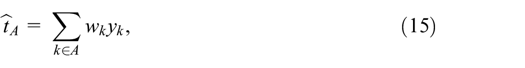
In this section, we construct the estimator of the total based on the non-probability sample under certain assumptions on its origin and present some of its properties. Treating the non-probability sample as random, we propose two variance estimators for this estimator. For comparison, the variance estimator by Chen et al. (2020) will be used.
We consider the Hájek-type estimator of the total :
which is based on the estimated pseudo-weights (a term introduced by Elliott (2009)) constructed for the non-probability sample elements.
2.1. Estimation of Pseudo-Weights
Let the number be the value of the pseudo-inclusion variable describing the belonging of the unit to the sample with the value if and otherwise. The model for the variable will be constructed using data , . Valliant (2009) notes that “a super-population model is a way of formalizing a relationship between a target variable and auxiliary data.” In our case, the role of the target variable is played by the variable , and we aim to establish its relationship with the auxiliary variables . We define random binary variables with observed values in the finite population . Each random variable is associated with the value of the study variable and the vector of auxiliary variable values . It is called a pseudo-inclusion indicator.
Random variables are non-identically distributed according to the distribution. The probability is called a propensity score. It is used to describe the probability that the population element belongs to the non-probability sample . We are going to apply a combination of the quasi-randomization approach (Elliott and Valliant 2017), using pseudo-inclusion probabilities , , together with the super-population framework (Hartley and Sielken 1975).
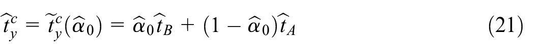
Construction of the non-probability sample-based estimator of the total Equation (1) needs some assumptions for the pseudo-inclusion indicators , similar to those in Wu (2022):
(A1) the pseudo-inclusion indicator and the variable value are independent given the covariates , , ;
(A2) all probabilities are positive: , ;
(A3) the finite population elements enter the non-probability sample with probabilities independently of each other, that is, the random variables and , , , are conditionally independent given and : .
Remark 1. Assumption (A2) ensures that all population elements can get to the non-probability sample, while assumption (A1) means a non-informative collection of the non-probability sample. Assumption (A3) implies that the non-probability sample size is random. Therefore, we consider the entry of the population elements into the sample approximated by a Poisson sampling design if (A2) and (A3) hold (Särndal et al. 1992, p. 85). We call it a Poisson pseudo-sampling design in the context of non-probability samples.
Remark 2. Assumptions (A1), (A2), and (A3) place significant restrictions on non-probability samples, which have prompted discussion among survey statisticians. For instance, a sample of volunteers may not be missing at random and thus fail to meet the assumption (A1). A shift away from strict reliance on assumption (A1) is emerging in some recent studies (Beaumont 2020; Kim and Morikawa 2023; Liu et al. 2024), although this shift is still in its early stages. Wu (2022) dedicated Section 7 of his article to revising the assumptions. In cases where (A2) is violated, he suggests considering the “stochastic under-coverage” scenario. Assumption (A3) covers only a subset of all possible non-probability samples. For example, non-probability samples based on incomplete administrative data may satisfy (A3), whereas network and quota samples often may not satisfy it.
To estimate the propensity scores under assumptions (A1) to (A3), a super-population parametric logistic regression model for distribution of is applied:
where is the vector of the real-valued parameters to be estimated. This model is fitted using the observed data specifying the non-probability sample . After the estimate of the model parameter is obtained, it is plugged in Equation (3) to get the estimated propensity scores
Then the estimator Equation (2) with the pseudo-weights is the IPW estimator of the total .
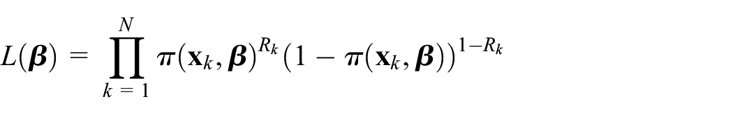
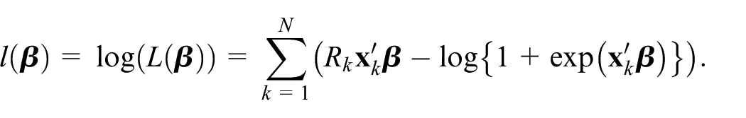
To estimate the vector parameter of the propensity scores , the maximum likelihood (ML) method is used. Due to the conditional independence of the indicators , , the ML method starts with defining the likelihood function
and its log-likelihood function
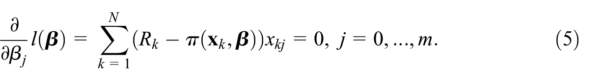
The function is continuous and has partial derivatives with respect to the components of of any order. The ML estimator of the parameter is found by solving the system of nonlinear equations
Since the estimator depends on the random variables , , it is itself a random variable. Replacing the random variables by their realizations , iterative methods are applied to solve approximately the equation system (5). The Newton–Raphson algorithm is frequently used for this purpose. Alternative ways to evaluate are based on estimating equations or calibration equations (Wu and Thompson 2020); however, the ML method is quite often used to fit the logistic regression model.
2.2. Variance Estimator Under the Randomized Propensity Scores
The variance of the estimator in (2) is studied in Chen et al. (2020) under the model Equation (2) for the propensity scores, where the ML estimator for the model parameter is assumed to be consistent and is treated as fixed when deriving the variance. We present asymptotic properties of . Utilizing these properties, the variance estimator for the IPW estimator of the population total , taking into account Poisson pseudo-sampling design and randomness in , is constructed.
The collection of the pseudo-inclusion indicators defines in our study a super-population.
Fahrmeir and Kaufmann (1985) presented the conditions that ensure the consistency and asymptotic normality of the ML estimators for the generalized linear models. Their result belongs to the field of classical statistics because they deal with a sample of independent observations.
In the paper, we use one of the generalized linear models–logistic regression model–for the super-population with the pseudo-inclusion indicators . In order to get the asymptotic properties of the logistic regression model parameter estimator, the result for the generalized linear model should be adapted. We herein use the adaptation performed in Fahrmeir and Tutz (2001), Section 2.2. To state the proposition, an additional technical assumption is required:
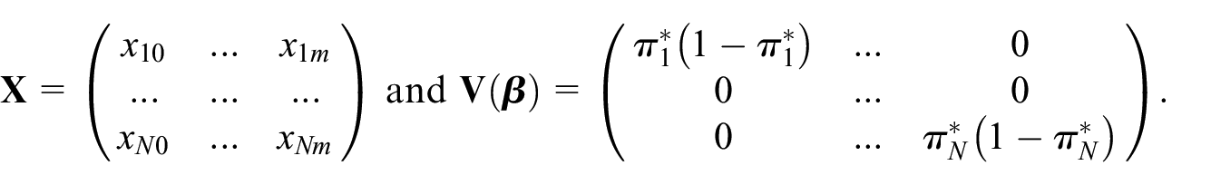
(A4) the components of the auxiliary vectors are uniformly bounded, and the matrix is of a full rank.
Proposition. If for the pseudo-inclusion indicators assumptions (A1) to (A4) are valid, then the random ML estimator obtained in the super-population for the parameter in Equation (3) has the following properties:
(i) The probability that exists and is unique tends to 1 for .
(ii) If denotes the “true” value of the logistic regression model parameter, then for we have in probability.
(iii) The random variable converges in distribution to the random variable , where and with the matrices
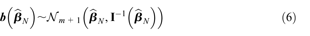
It follows from the proposition that for a large , the vector parameter can be approximated in the super-population by the values of the normally distributed random vector
with the density function of the multivariate normal distribution denoted further by . The realization of in the finite population should be followed by its inclusion in (6).
The IPW estimator is influenced by two dependent random components. Both components are caused by the non-probability sample collection process. One component is the direct effect of the pseudo-inclusion indicators , , on the estimated pseudo-weights and the resulting estimate of the population total. The random pseudo-inclusion indicators also lead to uncertainty in the ML estimator of the logistic regression model parameter . The second random component is the effect of the uncertainty in the ML estimator on the estimated pseudo-weights and resulting estimate of the finite population total. As noted in Remark 1, we consider the distribution of element pseudo-inclusion indicators as a Poisson pseudo-sampling design and denote it by . The distribution of , as well as the parameter itself, is approximated by the multivariate normal distribution of given in Equation (6) and is denoted by .
By replacing the value in the logistic regression model Equation (3) with the vector , we get the value , which approximates the propensity score . We aim to estimate an anticipated variance (Isaki and Fuller 1982), taking into account pseudo-sampling design and uncertainty in estimation.
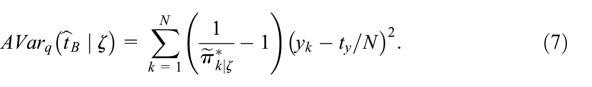
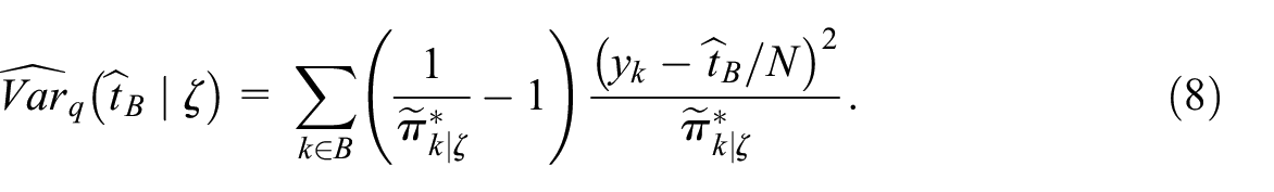
If the probabilities truthfully reflect the element belonging to the non-probability sample mechanism, then for a fixed value of –with the corresponding probabilities denoted by (here we adopt the notation of Särndal et al. (1992, Chapter 8.3))–the ratio estimator in Equation (2) based on the Poisson pseudo-sampling design is approximately unbiased, and its approximate conditional variance is
We estimate this variance by a modified formula appropriate for a Poisson sample (Z Liu and Valliant 2023):
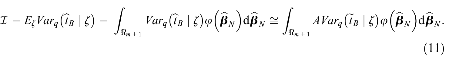
Taking into account two distributions, and , the anticipated variance of the estimator can be decomposed by the law of the total variance (Särndal et al. 1992, p. 136):
The subscript indicates that the variance and expectation are calculated according to the distribution of the indicators , and the subscript means the variance and expectation by the distribution . Due to the approximate unbiasedness of the estimator for a fixed value of the random variable , the first term in the relationship Equation (9) can be considered negligible. Then from Equation (9) we get the approximation
The expectation is by the multivariate normal distribution with the density and can be written as an integral and further approximated according to (10):
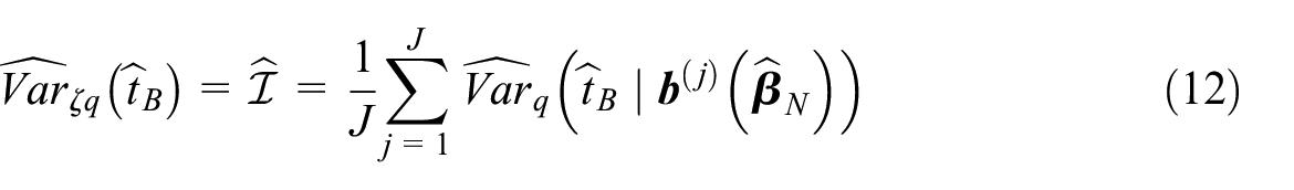
The Monte–Carlo approximation (Fahrmeir and Tutz 2001, Appendix A.5) of the integral gives us
for a large integer number of repetitions . Here the term is the estimator (8) of the variance with the propensity scores , , obtained by inserting the th simulated value into Equation (3). Expression Equation (12) means that the anticipated variance estimator equals empirical average of the design based estimators of variance with the estimates of the parameter spread around according to the distribution .
Let us summarize the simulation procedure to implement the estimator Equation (12) of variance Equation (9).
Variance estimation algorithm:
Compute the ML estimate for the parameter of the logistic regression model (3) replacing by . Calculate the propensity score estimates , , from (3).
Do the following calculations for each : simulate by Equation (6) using the estimates , ; calculate , , from Equation (3) using the simulated vector instead of ; evaluate the th constituent in Equation (12).
In what follows, we call the estimator Equation (12) a smooth variance estimator. Two more estimators of the variance are presented for comparison: an estimator by Chen et al. (2020), which considers the non-probability sample described only by the pseudo-inclusion indicators, and a bootstrap variance estimator, taking into account the randomness of the non-probability sample. They all are compared in the simulation study.
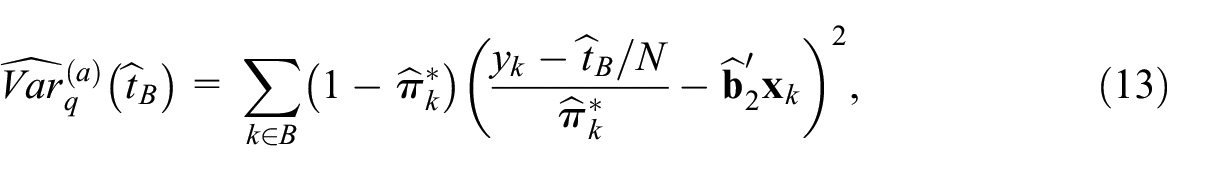
2.3. Variance Estimator Based on Asymptotic Variance
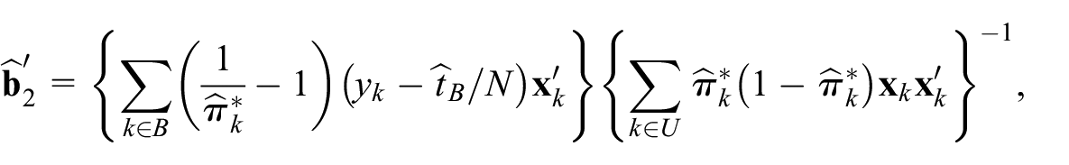
The IPW estimator of the population total with the ML estimator of the parameter also has been considered in Chen et al. (2020). These authors ascertained the properties of the IPW estimator given by Equation (2). They have shown that assuming the logistic regression model for the propensity scores under conditions (A1) to (A3) and some additional regularity conditions, the IPW estimator is asymptotically unbiased and derived its asymptotic variance. Chen et al. (2020) use this approximate variance to build a plug-in estimator of . Due to completely known auxiliary data, the variance estimator has a simpler expression (Burakauskaitė and Čiginas 2023):
where
given the non-probability sample .
The variance estimator Equation (13) considers the non-probability sample described only by pseudo-inclusion indicators.
2.4. Bootstrap Variance Estimator
Elliott and Valliant (2017) propose to use resampling methods to estimate the variances of the estimators based on the non-probability samples. They suggest that for the estimators like the IPW estimator in Equation (3), the bootstrap variance estimator should incorporate the variability in estimating the propensity scores and the variability caused by the sample selection mechanism in estimating the population total.
Elliott and Valliant (2017) mention that, given the estimates of pseudo-inclusion probabilities, design-based formulas may be used for point estimates and their variances. Mashreghi et al. (2016) presented the implementation of the bootstrap algorithm by Chauvet (2007) to estimate the variance of the IPW estimator Equation (2) for Poisson sampling. We have replaced the propensity scores by their estimates and applied this algorithm to estimate because this follows from assumption (A3). Moreover, to take into account the randomness of the non-probability sample, the bootstrap variance estimator is averaged over the distribution of the estimated propensity scores.
Bootstrap variance estimation algorithm:
1. Compute the ML estimate for the parameter of the logistic regression model Equation (3). Calculate the propensity score estimates , , from Equation (3).
2. Simulate by Equation (6) using the estimates , . Calculate , , from Equation (3) with the simulated vector in place of .
3. Repeat the pair , times for all to create , the fixed part of the bootstrap population.
4. To complete the bootstrap population, , construct the set by selecting independently elements from with the probability for the th pair. Denote the bootstrap population by , where is the th pair of this population corresponding to one of those in the initial sample . In addition, each inclusion probability , , is scaled by the factor , ensuring that their sum across the bootstrap population remains constant.
5. Draw the bootstrap sample elements independently from , with the probability for the th unit in .
6. Compute the bootstrap estimate by Equation (2) using the data .
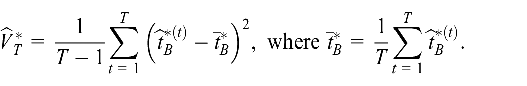
7. Repeat Steps 5 and 6 a large number of times, , to obtain . Calculate
8. Repeat Steps 4 to 7 a large number of times, , to get . Calculate the estimate
9. Repeat Steps 2 to 8 a large number of times, , to get . Calculate the estimate
of the variance for the IPW estimator Equation (2).
The asymptotic unbiasedness of this variance estimator, based on estimated pseudo-inclusion probabilities, remains unestablished and could be a focus of future research.
3. Design-Based and Composite Estimators of the Total and Estimation of Their Variances
The mechanism by which an element is included in the non-probability sample is unknown. Therefore, even a carefully constructed IPW estimator may not sufficiently correct the selection bias of this sample. If an additional, albeit much smaller, independently selected probability sample is available in which the study variable is observed, it provides supplementary information about the population and can be used to deal with the possibly biased IPW estimator Equation (2). For this purpose, we integrate both samples through a linear combination of the IPW and design-based estimators.
Let us assume that, independently of sample , a probability sample is selected from the same population according to the sampling design , and the values , , are observed. The samples and may overlap. Let be the selection indicator for a unit , selected to the sample with the value if and otherwise.
The design-based estimator of the population total is defined as:
which is at least approximately unbiased, according to the randomness induced by the probability sampling design . This estimator may be the Horvitz–Thompson estimator with exactly or approximately known inclusion probabilities and weights , , or another estimator using auxiliary data (Särndal et al. 1992); or the Hájek estimator
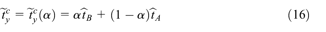
The integration of both samples–non-probability and probability–is done through the composite estimator of the total :
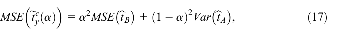
with the coefficient minimizing the mean squared error (MSE) of the estimator . Since the samples and are selected independently, the estimators and are independent as well, implying that . Assuming further that the estimator is unbiased, the MSE can be expressed as
where with a possibly non-negligible bias component
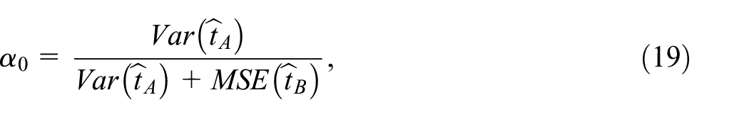
The minimum value of the function in Equation (17) is attained at for
and the coefficient has to be estimated from the data available. Here, the variance is readily estimated using the standard design-based methods (Särndal et al. 1992; Wolter 2007), while the estimation of the variance depends on the specific choice of the pseudo-weights in Equation (2) and other assumptions as considered in Section 2. If the pseudo-weight construction method correctly reflects the population unit involvement in the non-probability sample mechanism, then an approximately unbiased estimator can be expected. Otherwise, the estimator can be significantly biased. We further propose an estimator of the bias to evaluate the optimal coefficient Equation (19) properly.
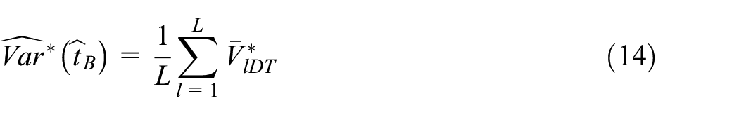
Let us study the variability of the composite estimator Equation (16) of the population total. Three different estimators of the variance for the IPW estimator Equation (2) are considered: the new estimator given by Equation (12), the estimator of Chen et al. (2020) given by Equation (13), and the bootstrap estimator from Equation (14). Denote further by any of these estimators.
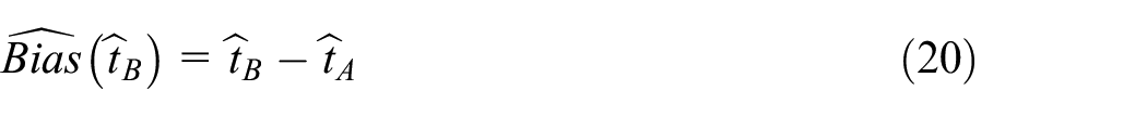
Since the study variable is observed in the probability sample , the true population total in the expression of the bias Equation (18) is at least approximately unbiasedly estimated using , while is taken as the estimator of the population parameter . Then the estimator
of the bias is at least approximately unbiased, with the variance due to the independence of the estimators and . The bias estimator Equation (20) is suggested also by Elliott and Haviland (2007).
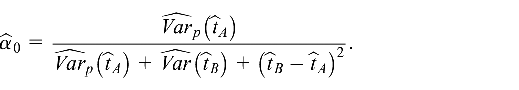
Then, after the estimator of the variance of the design-based estimator in Equation (15) is chosen, the optimal coefficient in Equation (19) for the composition Equation (16) is estimated by
Finally, the composite estimator
of the population total is obtained, and its MSE is estimated by
This formula is derived by inserting into (17). The more the estimator is biased or highly fluctuating, the lower its coefficient in the composition Equation (21). The efficiency of the composite estimator Equation (21) of for different choices of the variance estimator is examined in the simulation study.
The estimator , based on the non-probability sample, is biased but has low variance. In contrast, the estimator , supported by the probability sample, is unbiased but exhibits relatively high variance. By combining these two estimators, the composite estimator “borrows strength” from both, similar to techniques used in small area estimation (Rao and Molina 2015). This approach mitigates the weaknesses of the individual components, leading to an estimator with comparatively lower variance and reduced bias. The effectiveness of this method is demonstrated in the simulation study.
4. Numerical Experiment
A numerical study aims to compare the estimators considered, show the alternation of their accuracy when the researcher fails to specify the propensity score model precisely enough and demonstrate the composite estimator’s usefulness regardless of the probability sample size. The essence of the numerical experiment is to simulate the problem environment by repeatedly generating the non-probability and probability samples, estimating the population total and the variances of its estimators by several methods, and studying the distributions of the estimators obtained. The results allow us to compare the accuracy of the estimators and show the conditions under which any of these estimators can be efficient.
4.1. Simulation Data
The data set used in the simulations is constructed using three data sets (sources) with the same record identifier. The first is the probability sample data set from the Lithuanian Information and Communication Technology (ICT) survey, with the binary study variable indicating whether the enterprise has a website. For its selection, stratified simple random sampling is used. The values of other variables, such as the number of employees and the indicators of economic activity, are known for the whole survey population of size . One more completely known auxiliary variable is derived from the second, web-scraped data set. This binary variable approximates the study variable quite well. The third data set, containing values of the variable , is provided by a private company. This data source is a voluntary non-probability sample covering about of the survey population.
The pseudo-real population of the real size is constructed by linking these three data sets. The values in the probability survey sample are supplemented with observations in the non-probability sample, and further information is gathered about the remaining unknown values. In the population obtained, the contingency coefficient between and , measuring the relationship strength between these variables, equals (while the maximal possible value of the contingency coefficient for frequency table is ). The auxiliary variables include the web-scraped variable , the number of employees, and some variables indicating economic activity.
4.2. Simulation Procedure
The simulation procedure consists of the following steps:
The logistic regression model Equation (3) is fitted using the linked non-probability sample. Then, the estimates Equation (4) of the propensity scores are obtained for all population elements. They are used further as Poisson sample selection probabilities.
Two independent samples are constructed from the pseudo-real population . The first is a stratified simple random sample mimicking an original ICT survey sampling design. For simulation purposes, two versions of the probability samples of different sizes are considered: sample of size and a smaller sample of size . Two different approaches are employed to collect the second sample . In the first case, sample is selected using the Poisson sampling design, with the selection probabilities obtained in Step 1, with the expected sample size equal to . In the second case, a stratified simple random sample of size is selected after the pseudo-real population is divided into strata according to the enterprise size (5 strata by the number of employees).
Three combinations of probability and non-probability samples are considered:
(a) Case 1. is used as sample , and is used as sample . This combination corresponds to an existing situation investigating whether integrating both samples improves estimation accuracy.
(b) Case 2. is used as sample , and is used as sample . This combination uses a probability sample that is three times smaller (cheaper), allowing us to investigate the usefulness of the probability sample in reducing the biases of the estimates obtained from the non-probability sample.
(c) Case 3. is used as sample , and is used as sample . This case considers a scenario where the probability sample size is small, and the non-probability sample is represented by a sample that does not satisfy assumptions (A1) and (A3) and has a structure that is not harmonized with the estimation methodology.
3. Using the generated samples and , the following estimates are calculated:
(a) A set of covariates is chosen from the collection , and a logistic regression model (3) is applied to the non-probability sample to get the estimates , , of the propensity scores. These estimates are then used to evaluate the estimator of the population total and three estimators of the variance :
•the proposed smooth estimator Equation (12), calculated with ;
•the bootstrap estimator Equation (14) with parameters , , and ;
(b) Using the probability sample , the population total is estimated by applying the regression estimator based on the auxiliary variable .
(c) The Hájek estimator of the total, calculated from sample , serves as a benchmark in the simulations.
(d) The composite estimators Equation (21) of are calculated using each of the estimates of variance listed in (a).
(e) The naive estimator of is calculated, where is the size of sample .
4. Steps 2 and 3 are repeated times. The numerical characteristics, like the average over the repetitions, are calculated for each estimator of interest.
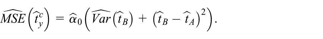
The selection of covariates for the logistic regression model in Step 3 is needed to imitate a situation where the data are not well-known to the researcher. The following three logistic regression models of different quality levels are used:
I The model includes all possible covariates that are the same as those used to estimate the pseudo-inclusion probabilities in Step 1.
II The model incorporates all covariates, except for the number of employees, which has a smaller impact on the values of the study variable than the variable
III The model includes all the covariates without the variable
The quality comparison of the logistic regression models is performed using the Akaike information criterion and presented in Table 1. The model with a lower value of this criterion fits the data better.
Quality Classification of Logistic Regression Models.
Model
Akaike criterion
Model quality
Model I
17,504
Strong
Model II
17,825
Weak
Model III
18,742
Poor
According to the values of the Akaike criterion, the logistic regression models are classified as strong, weak, and poor.
4.3. Simulation Results
The numerical characteristics of the simulated estimates, namely their empirical means, biases, standard deviations, and root mean square errors (), are obtained for both estimates of the population total and variance: where , , are the realizations of , while the population parameter denotes or .
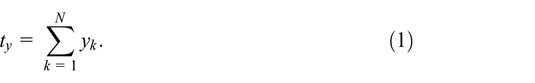
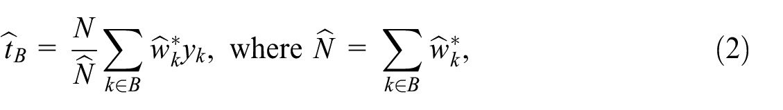
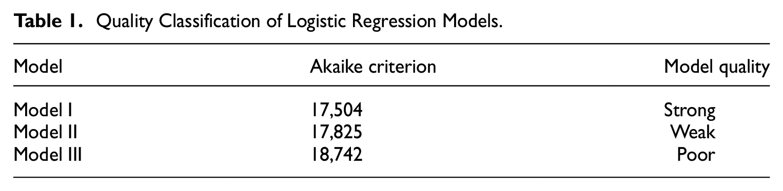
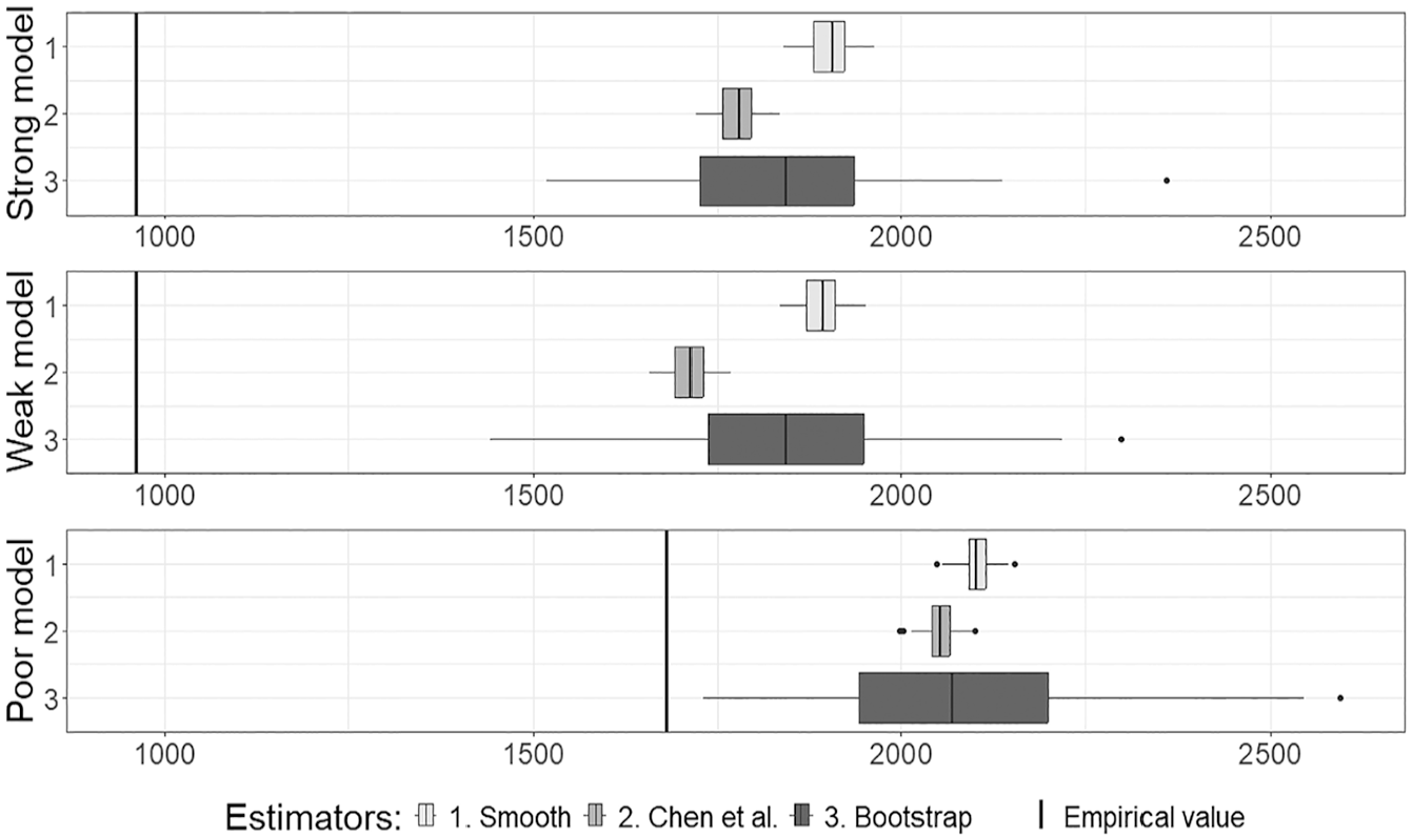
First of all, the estimators of the variance based on the non-probability samples used in Cases 1 to 3 are graphically overviewed. The variance estimates are the same for Cases 1 and 2 because they are applied to the same non-probability sample and are presented in Figure 1. For Case 3, the variance estimates are presented in Figure 2.
Variance estimates for the estimator in Cases 1 and 2.
Variance estimates for the estimator in Case 3.
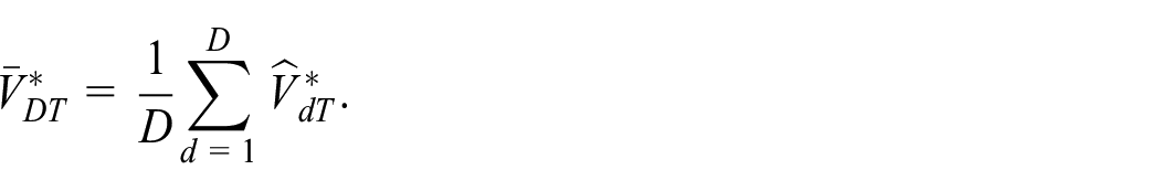
The vertical lines in Figures 1 and 2 represent the empirical variance
where , , are the IPW estimates obtained by (2), and is their average. The proposed smooth variance estimator is expected to be greater than the empirical variance because it accounts for both the variability in estimating the propensity scores and the variability caused by the sample collection mechanism in estimating the population total. In contrast, the empirical variance considers the non-probability sample described only by pseudo-inclusion indicators.
Considering Figure 1, for the poor model, all variance estimators, including the proposed smooth estimator Equation (12), are higher than the empirical variance Equation (22), behave similarly and have higher variability compared to other model cases. For the strong and weak model cases, the smooth estimator behaves similarly to the bootstrap estimator, while the variance estimates by Chen et al. (2020) are, on average, lower.
In Case 3 (Figure 2), as compared to Cases 1 and 2 (Figure 1), we observe the same trends in the variance estimates, except for the fact that the bootstrap variance estimates have a much wider spread than other variance estimates. This difference may be because, in Case 3, the non-probability sample does not satisfy assumptions (A1) and (A3), and the bootstrap variance estimation is more sensitive to this factor due to resampling.
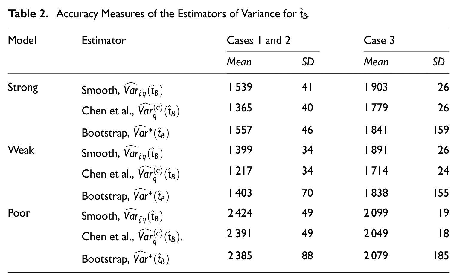
The means and standard deviations of the variance estimates in Table 2 numerically express the situation presented in Figures 1 and 2.
Accuracy Measures of the Estimators of Variance for .
Model
Estimator
Cases 1 and 2
Case 3
Strong
Smooth,
Chen et al.,
Bootstrap,
Weak
Smooth,
Chen et al.,
Bootstrap,
Poor
Smooth,
Chen et al., .
2 391
49
Bootstrap,
The results in Table 2 confirm that in Case 3, the of the bootstrap variance estimator is comparatively large. The Chen et al. (2020) variance estimator consistently yields the lowest mean estimates across all models and cases, as it does not account for the variability caused by the sample collection mechanism. The smooth variance estimator generally produces higher mean estimates, while its remains similar to that of the Chen et al. (2020) estimator. This suggests that incorporating two sources of variability increases the value of the variance estimator without inflating its variability.
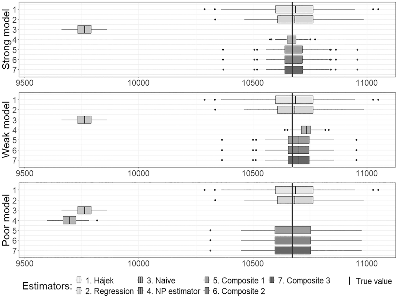
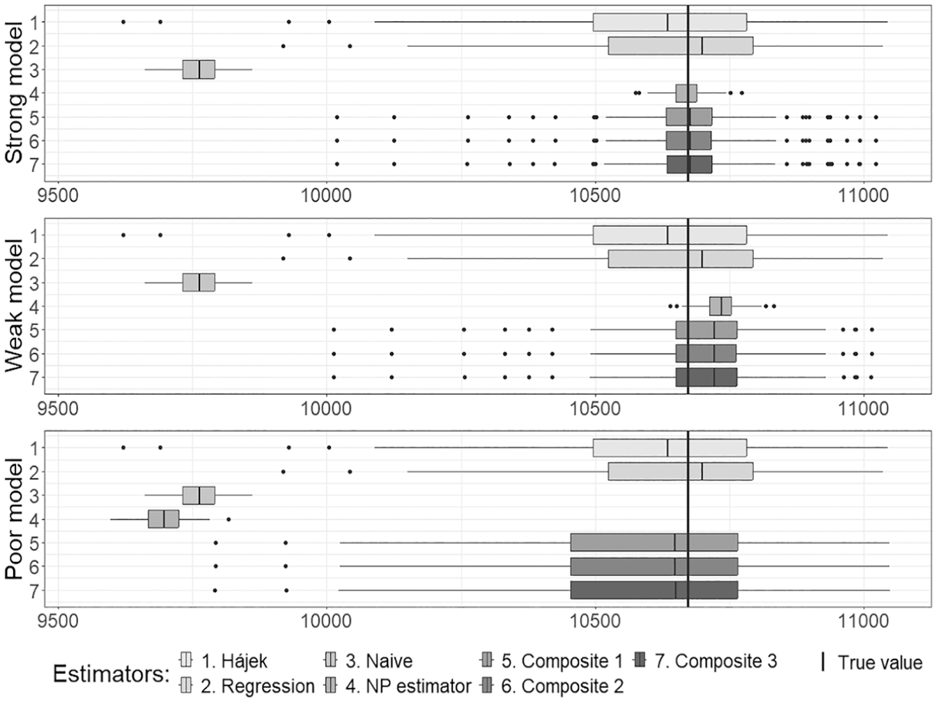
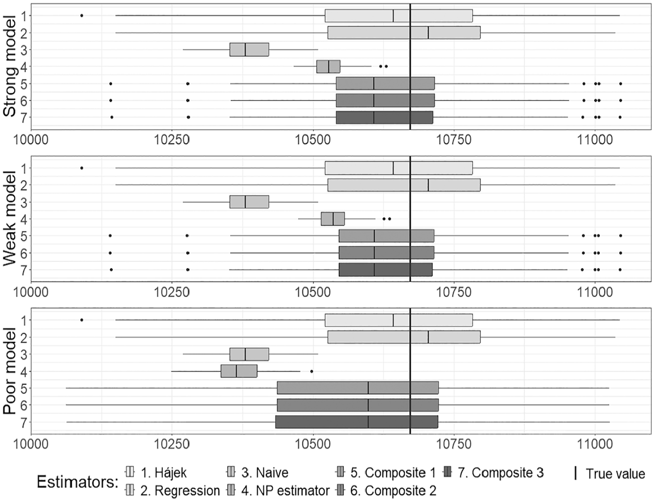
The results for all estimators of the population total are presented in Figures 3 to 5, which correspond to Cases 1 to 3. Here Composite 1 denotes the composite estimator (21), with the coefficient using the smooth estimator of variance, Composite 2 uses the variance estimator of Chen et al. (2020), and Composite 3 is based on the bootstrap variance estimator. The estimator is denoted by NP.
Estimates of the population total in Case 1.
Estimates of the population total in Case 2.
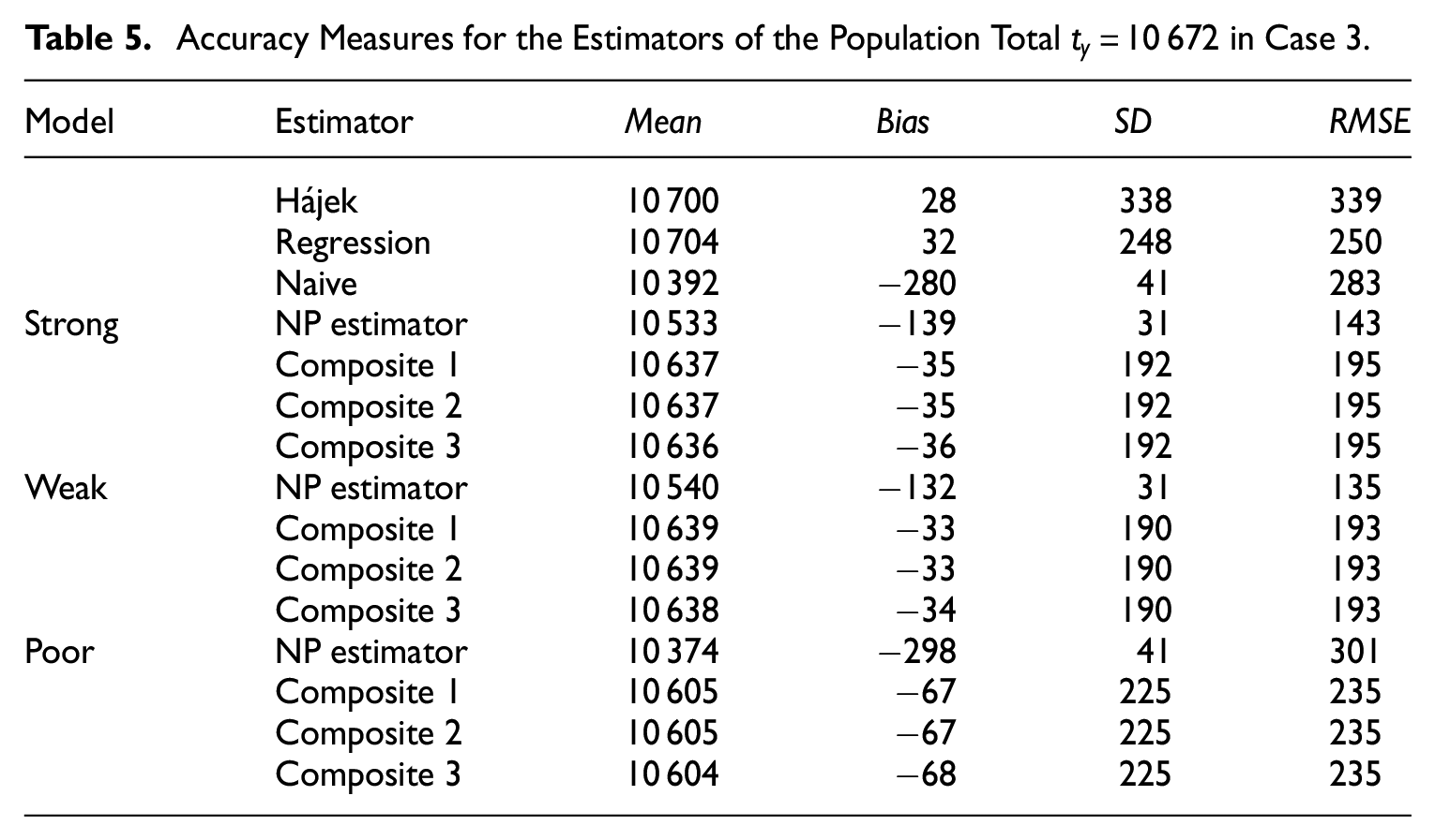
Estimates of the population total in Case 3.
Figures 3 to 5 depict the positions of the simulated estimates relative to the known true value of the population total, indicated by a straight line. The naive estimates of the total, using the non-probability sample as a simple random sample from the population, exhibit a significant bias across all cases. The estimates (NP estimates) demonstrate a narrow spread for all cases, regardless of which logistic regression model is utilized. In Cases 1 and 2, where the role of the non-probability sample is played by a sample selected using the Poisson sampling design with the pseudo-selection probabilities obtained in Step 1, the estimator is nearly unbiased for the strong model, exhibits some bias for the weak model, and demonstrates a significant bias for the poor model. When the role of the non-probability sample is played by a sample selected in a different manner in Case 3, the bias of the estimator decreases (compared to the naive estimator); nevertheless, it still remains considerable. The behavior of composite estimates remains consistent regardless of the method used to estimate the optimal weight . In all cases, their spread is narrower than that of the regression estimates applied to the probability sample for the strong and weak models; however, they do not outperform regression estimates when the quality of the logistic regression model for the propensity scores is poor.
In the case where is used as sample and is used as sample , the same tendencies as in Figure 5 are observed. Due to the larger probability sample size and the lower variance of the unbiased estimator, the spread of the estimates is slightly narrower. The figure for this case is not shown.
The smooth variance estimator is efficient when assumptions (A1) and (A3) for the pseudo-inclusion indicators hold, and the logistic regression model used to estimate pseudo-inclusion probabilities, , is sufficiently strong (well specified). As the quality of this model declines, the bias in the smooth variance estimator increases. However, in our application, a composite estimator alleviates this issue across any variance estimator, as the bias of the estimator is notably larger than its variance due to the relatively large non-probability sample.
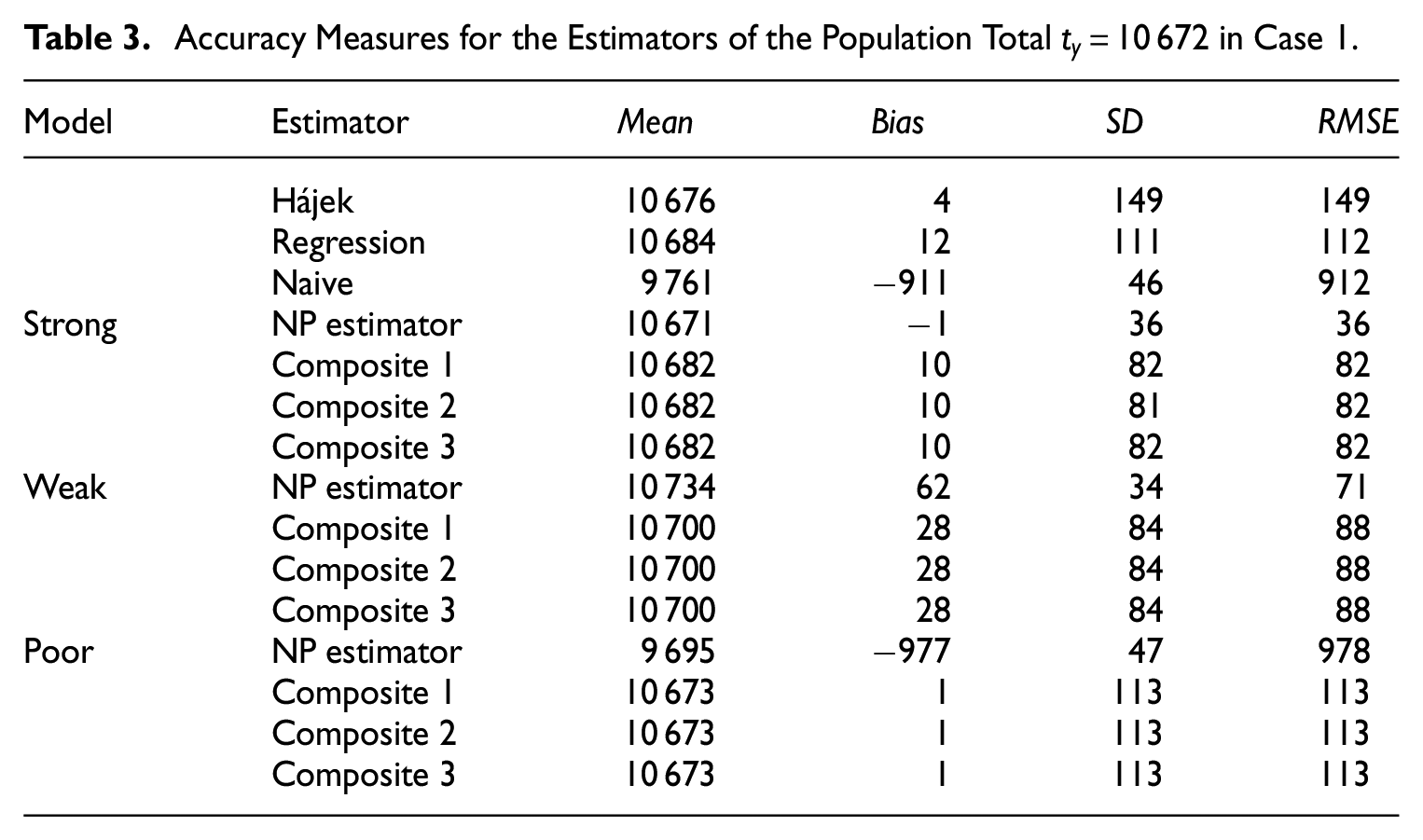
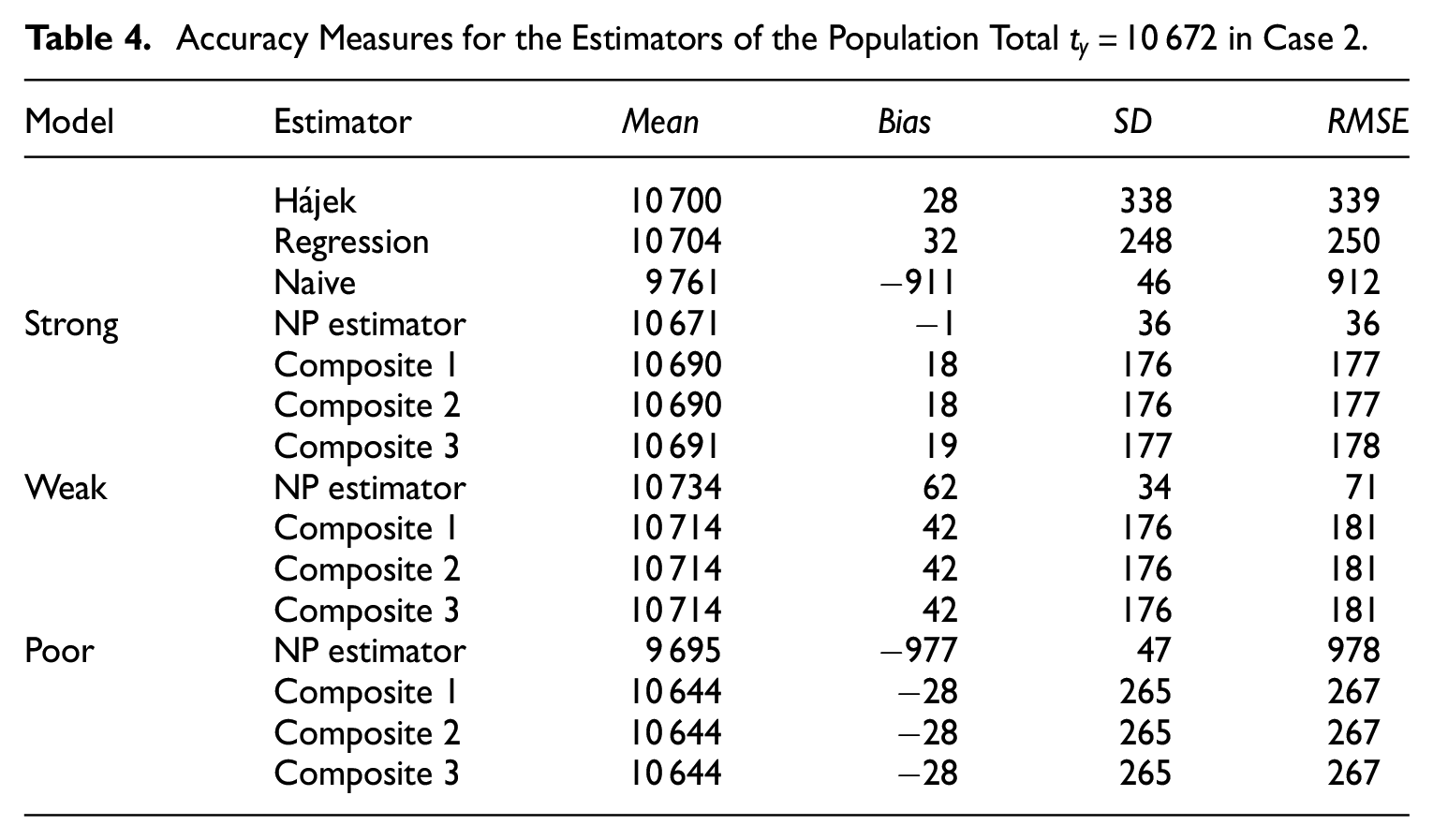
The numerical summary of Figures 3 to 5 is provided in Tables 3 to 5, respectively.
Accuracy Measures for the Estimators of the Population Total in Case 1.
Model
Estimator
Hájek
Regression
Naive
Strong
NP estimator
Composite 1
Composite 2
Composite 3
Weak
NP estimator
Composite 1
Composite 2
Composite 3
Poor
NP estimator
Composite 1
Composite 2
Composite 3
Accuracy Measures for the Estimators of the Population Total in Case 2.
Model
Estimator
Hájek
Regression
Naive
Strong
NP estimator
Composite 1
Composite 2
Composite 3
Weak
NP estimator
Composite 1
Composite 2
Composite 3
Poor
NP estimator
Composite 1
Composite 2
Composite 3
Accuracy Measures for the Estimators of the Population Total in Case 3.
Model
Estimator
Hájek
Regression
Naive
Strong
NP estimator
143
Composite 1
10 637
Composite 2
Composite 3
Weak
NP estimator
Composite 1
Composite 2
Composite 3
Poor
NP estimator
Composite 1
Composite 2
Composite 3
The accuracy measures in Tables 3 to 5 corroborate the observed behavior (refer to Figures 3–5, respectively) of all three composite estimators, indicating their insensitivity to the choice of the variance estimator based on the non-probability sample. For the high-quality (strong) logistic regression model, the NP estimator based solely on the non-probability sample achieves the lowest for all cases. However, this estimator exhibits a significant bias under the poor model. Simulation results demonstrate that composite estimators are much more stable due to the bias of the NP estimator incorporated into their expression. Even with a poor model for the propensity scores, it is possible to obtain an almost unbiased composite estimator, albeit with an comparable to that of the regression estimator applied to the probability sample. In the case of the weak model, composite estimators exhibit a smaller bias than the NP estimator, but their s are higher. It is noteworthy that the accuracy characteristics of composite estimators remain consistent regardless of the differences observed between the variance estimates for the NP estimator of the total (see Table 2).
5. Conclusions and Discussion
The estimates of the population total based on a non-probability sample usually are biased. The nature of the non-probability sample is typically unknown; however, there is no reason to presume that it is not random in some specific applications. One of the ways to decrease the bias of the estimator of the total using a non-probability sample is to assume the probabilistic nature of this sample and use it for estimation and inferences.
The assumption of an independent entry of elements into the non-probability sample with probabilities estimated by the propensity scores from the logistic regression model is well-suited for this purpose. The accuracy of the IPW estimator of the total depends on how well the propensity score model is specified. As the simulation results show, if the model adequately reflects the mechanism of formation of a non-probability sample, then the IPW estimator may have an insignificant bias. Otherwise, the IPW estimator is biased, and a probability sample with an approximately unbiased estimator of the total is needed. The proposed composite estimator with the bias component included in its coefficient gives nearly unbiased estimates in the case of any logistic regression model for the propensity scores.
However, it is not enough to assume a probabilistic sample pseudo-selection mechanism for a non-probability sample. One should also consider the possible randomness in this mechanism, as it is done for the proposed smooth estimator of variance. This estimator averages the known estimator of the variance of the ratio estimator over the distribution of propensity score estimates. According to the simulation results, if the model for the propensity scores is not poor, then this average value is close to the value of the bootstrap estimator of variance, and its spread is not wider than that for the bootstrap. The advantage of the smooth variance estimator over the bootstrap variance estimator becomes even more pronounced when the non-probability sample formation mechanism significantly differs from that described by the logistic regression model.
In our setup, the values of the study variable are available in both non-probability and probability samples. In practice, if the collection of probability sample data is expensive, then a small probability sample may be selected and utilized through composite estimation to decrease the bias of the IPW estimate. The simulation study demonstrates that the composite estimator is more efficient than the estimator based on a small probability sample and performs comparably to the estimator based on a large probability sample. Moreover, regardless of the probability sample size, composite estimators significantly improve the accuracy of other estimators of the population total if the underlying logistic regression model is well-specified.
Further research could focus on integrating probability and non-probability samples over time, addressing non-sampling errors, and estimating nonlinear population parameters while accounting for the randomness of the non-probability sample.
Footnotes
Acknowledgements
We sincerely thank three anonymous Referees and a Guest Editor for their valuable comments, which have brought attention to important details and significantly improved the quality of this article.
Funding
The authors received no financial support for the research, authorship, and/or publication of this article.
ORCID iDs
Andrius Čiginas
Danutė Krapavickaitė
Vilma Nekrašaitė-Liegė
Received: July 6, 2023
Accepted: March 11, 2025
References
1.
BeaumontJ.-F.2020. “Are Probability Surveys Bound to Disappear for the Production of Official Statistics?”Survey Methodology46 (1): 1–28.
2.
BurakauskaitėI.ČiginasA.2023. “An Approach to Integrating a Non-Probability Sample in the Population Census.” Mathematics11 (8): 1782–95. DOI: https://doi.org/10.3390/math11081782.
3.
ChauvetG.2007. “Méthodes de bootstrap en population finie.” PhD thesis, Université de Rennes2.
4.
ChenY.LiP.WuC.2020. “Doubly Robust Inference with Nonprobability Survey Samples.” Journal of the American Statistical Association115 (532): 2011–21. DOI: https://doi.org/10.1080/01621459.2019.1677241.
ElliottM. N.HavilandA.2007. “Use of a Web-Based Convenience Sample to Supplement a Probability Sample.” Survey Methodology33 (2): 211–5.
7.
ElliottM. R.2009. “Combining Data from Probability and Non-Probability Samples Using Pseudo-Weights.” Survey Practice2 (6): 1–7. DOI: https://doi.org/10.29115/SP-2009-0025.
FahrmeirL.KaufmannH.1985. “Consistency and Asymptotic Normality of the Maximum Likelihood Estimator in Generalized Linear Models.” The Annals of Statistics13 (1): 342–68. DOI: https://doi.org/10.1214/aos/1176346597.
HartleyH. O.SielkenR. L.Jr.1975. “A ‘Super-Population Viewpoint’ for Finite Population Sampling.” Biometrics31 (2): 411–22. DOI: https://doi.org/10.2307/2529429.
12.
IsakiC. T.FullerW. A.1982. “Survey Design Under the Regression Superpopulation Model.” Journal of the American Statistical Association37 (377): 89–96. DOI: https://doi.org/10.2307/2287773.
13.
JapecL.KreuterF.BergM.BiemerP.DeckerP.LampeC.LaneJ.O’NeilCUsherA.2015. “Big Data in Survey Research: AAPOR Task Force Report.” Public Opinion Quarterly79 (4): 839–80. DOI: https://doi.org/10.1093/poq/nfv039.
14.
KimJ. K.MorikawaK.2023. “An Empirical Likelihood Approach to Reduce Selection Bias in Voluntary Samples.” Calcutta Statistical Association Bulletin75 (1): 8–27. DOI: https://doi.org/10.1177/00080683231186488.
15.
KimJ. K.TamS.-M.2021. “Data Integration by Combining Big Data and Survey Sample Data for Finite Population Inference.” International Statistical Review89 (2): 382–401. DOI: https://doi.org/10.1111/insr.12434.
16.
KimJ. K.WangZ.2019. “Sampling Techniques for Big Data Analysis.” International Statistical Review87 (1): 177–91. DOI: https://doi.org/10.1111/insr.12290.
17.
LiuA.-C.ScholtusS.de WaalT.2023. “Correcting Selection Bias in Big Data by Pseudo-Weighting.” Journal of Survey Statistics and Methodology11 (5): 1181–203. DOI: https://doi.org/10.1093/jssam/smac029.
LiuZ.ValliantR.2023. “Investigating an Alternative for Estimation from a Nonprobability Sample: Matching Plus Calibration.” Journal of Official Statistics39 (1): 45–78. DOI: https://doi.org/10.2478/jos-2023-0003.
20.
LohrS. L.RaghunathanT. E.2017. “Combining Survey Data with Other Data Sources.” Statistical Science32 (2): 293–312. DOI: https://doi.org/10.1214/16-STS584.
21.
LothianJ.HolmbergA.SeybA.2019. “An Evolutionary Schema for Using ‘It-Is-What-It-Is’ Data in Official Statistics.” Journal of Official Statistics35 (1): 137–65. DOI: http://dx.doi.org/10.2478/JOS-2019-0007.
22.
MashreghiZ.HazizaD.LégerC.2016. “A Survey of Bootstrap Methods in Finite Population Sampling.” Statistical Survey10: 1–52. DOI: https://doi.org/10.1214/16-ss113.
23.
MengX.-L.2018. “Statistical Paradises and Paradoxes in Big Data (I): Law of Large Populations, Big Data Paradox, and the 2016 US Presidential Election.” The Annals of Applied Statistics12 (2): 685–726. DOI: https://doi.org/10.1214/18-aoas1161sf.
24.
RaoJ. N. K.2021. “On Making Valid Inferences by Integrating Data from Surveys and Other Sources.” Sankhya B83 (1): 242–72. DOI: https://doi.org/10.1007/s13571-020-00227-w.
25.
RaoJ. N. K.MolinaI.2015. Small Area Estimation. Hoboken, NJ: Wiley.
26.
RuedaM.Pasadas-del-AmoS.RodríguezB.Castro-MartínL.Ferri-GarcíaR.2023. “Enhancing Estimation Methods for Integrating Probability and Nonprobability Survey Samples with Machine-Learning Techniques. An Application to a Survey on the Impact of the COVID-19 Pandemic in Spain.” Biometrical Journal65 (2): 1–19. DOI: https://doi.org/10.1002/bimj.202200035.
27.
SalvatoreC.2023. “Inference with Non-Probability Samples and Survey Data Integration: A Science Mapping Study.” Metron81 (1): 83–107. DOI: http://dx.doi.org/10.1007/s40300-023-00243-6.
TamS.-M.KimJ. K.2018. “Big Data Ethics and Selection-Bias: An Official Statistician’s Perspective.” Statistical Journal of the IAOS34 (4): 577–88. DOI: https://doi.org/10.3233/sji-170395.
ValliantR.2009. “Model-Based Prediction of Finite Population Totals.” Handbook of Statistics: Sample Surveys: Inference and Analysis29B: 11–31. DOI: https://doi.org/10.1016/S0169-7161(09)00223-5.
YangS.KimJ. K.2020. “Statistical Data Integration in Survey Sampling: A Review.” Japanese Journal of Statistics and Data Science3: 625–50. DOI: https://doi.org/10.1007/s42081-020-00093-w.
36.
YangS.KimJ. K.SongR.2020. “Doubly Robust Inference When Combining Probability and Non-Probability Samples with High Dimensional Data.” Journal of the Royal Statistical Society: Series B (Statistical Methodology)82 (2): 445–65. DOI: https://doi.org/10.1111/rssb.12354.
37.
ZhangL.-C.2019. “On Valid Descriptive Inference from Non-Probability Sample.” Statistical Theory and Related Fields3 (2): 103–13. DOI: https://doi.org/10.1080/24754269.2019.1666241.