
Abstract
We used Monte Carlo simulations to compare the performance of marginal structural models (MSMs) based on weighted univariate generalized linear models (GLMs) to estimate risk differences and relative risks for binary outcomes in observational studies. We considered four different sets of weights based on the propensity score: inverse probability of treatment weights with the average treatment effect as the target estimand, weights for estimating the average treatment effect in the treated, matching weights and overlap weights. We considered sample sizes ranging from 500 to 10,000 and allowed the prevalence of treatment to range from 0.1 to 0.9. We examined both the robust variance estimator when using generalized estimating equations with an independent working correlation matrix and a bootstrap variance estimator for estimating the standard error of the risk difference and the log-relative risk. The performance of these methods was compared with that of direct weighting. Both the direct weighting approach and MSMs based on weighted univariate GLMs resulted in the identical estimates of risk differences and relative risks. When sample sizes were small to moderate, the use of an MSM with a bootstrap variance estimator tended to result in the most accurate estimates of standard errors. When sample sizes were large, the direct weighting approach and an MSM with a bootstrap variance estimator tended to produce estimates of standard error with similar accuracy. When using a MSM to estimate risk differences and relative risks, in general it is preferable to use a bootstrap variance estimator than the robust variance estimator. We illustrate the application of the different methods for estimating risks differences and relative risks using an observational study on the effect on mortality of discharge prescribing of a beta-blocker in patients hospitalized with acute myocardial infarction.
Keywords
Introduction
Propensity score weighting is frequently used to estimate the effects of treatments and interventions when using observational data. In a setting with a binary treatment or intervention (e.g. treatment vs control), the propensity score is the probability of a subject being treated (vs receiving the control) conditional on the subject's observed baseline covariates. 1 Propensity score weighting entails constructing weights that are derived from the propensity score. Several sets of propensity score-based weights have been proposed, each of which has a different target estimand. The original set of propensity score-based weights, referred to as inverse probability of treatment weights, are equal to the inverse of the probability of receiving the treatment that subject received. 2 These weights allow one to estimate the average treatment effect (ATE). Alternative sets of weights have as target estimand the average treatment effect in the treated (ATT) or the effect of treatment in those subjects for whom there is equipoise in treatment selection (i.e. those subjects whose propensity score is close to 0.5).3–6 Note that the different estimands should not be seen as interchangeable and the choice of target estimand should be based on the research question of interest. 7
Binary outcomes (e.g. death within 30 days or symptom resolution) are common in clinical and health services research.
8
When outcomes are binary, the effect of treatment can notably be quantified using four metrics: the risk difference, the relative risk, the number needed to treat (NNT), and the odds ratio. Let Y denote the binary outcome, with Y = 1 denote the occurrence of the outcome (e.g. death occurred within 30 days) and Y = 0 denoting the absence of the outcome (e.g. death did not occur within 30 days) and let Z denote treatment status (Z = 0 control vs Z = 1 treated). Let P1 and P0 denote the probability of the outcome in treated and control subjects, respectively: P1 = Pr(Y = 1|Z = 1) and P0 = Pr(Y = 1|Z = 0). The risk difference and the relative risk are defined as P1–P0 and P1/P0, respectively. The NNT is the reciprocal of the risk difference and is equal to the number of subjects who must be treated to avoid one outcome event. The odds ratio is equal to
Several clinical commentators have suggested that, at the very least, absolute measures of treatment effect be reported to complement relative measures of effect. Laupacis and colleagues suggested that the risk difference is superior to the relative risk because it incorporates both baseline risk and the reduction in risk due to treatment. 9 However, they suggest that the NNT is more clinically interpretable. This is echoed by Cook and Sackett who suggested that the NNT is more meaningful for clinical decision making. 10 Sinclair and Bracken suggest that risk differences, relative risks, and the NNT be reported when addressing clinically important questions. 11 Sackett, Deeks, and Altman suggested that the odds ratio not be used as a measure of effect in randomized controlled trials (RCTs). 12 The CONSORT statement for the reporting of RCTs recommends that both relative and absolute measures of treatment effects be reported in RCTs with dichotomous outcomes (Statement 17b). 13 For RCTs, the BMJ (formerly the British Medical Journal) requires that authors report the absolute event rate in each arm, the relative risk reduction, and the NNT. 14 The measures of effect reported in observational studies should reflect those reported in comparable RCTs. 15 Thus, it is important to assess the performance of statistical methods for estimating risk differences and relative risks in observational studies.
When using propensity score-based weighting there are two primary approaches that can be used to estimate the effect of treatment when outcomes are binary. First, one can compute the weighted proportion of success or failures in treated and control subjects separately. The risk difference and the relative risk can be computed as the difference and ratio of these two weighted proportions, respectively. Different authors have described asymptotic variance estimators for risk differences and relative risks.16,17 A recent study examined the use of the bootstrap when using propensity score-based weights with continuous and binary outcomes. 18 When sample sizes were ≤ 1000 and the ATE was the target estimand, then the use of the bootstrap resulted in estimates of standard error that were more accurate than the asymptotic variance estimates. Second, one can fit a marginal structural model (MSM), in which the binary outcome is regressed on an indicator variable denoting treatment status using a weighted regression model.19,20 Robins and colleagues suggested that weighted generalized linear models (GLMs) with a binomial distribution and identity link can be used to estimate risk differences, weighted GLMs with a binomial distribution and log link can be used to estimate relative risks, while a weighted GLM with a binomial distribution and a logistic link function (i.e. a weighted logistic regression model) can be used to estimate odds ratios. 20 Joffe and colleagues used a weighted logistic regression model to estimate a marginal odds ratio for a binary outcome. 19 Both sets of authors suggested that the variance of the estimated treatment effect can be estimated using estimating equation methods with a robust variance estimator, with Robins and colleagues noting that the resultant estimated confidence intervals will be conservative (i.e. the true coverage rate will be at least as large as the advertised rate).19,20 Neither set of authors evaluated the performance of these methods, either in terms of bias or the accuracy of variance estimation. Despite Robins and colleagues suggesting that marginal risk differences and marginal relative risks can be estimated using an appropriate MSM, it appears that this is rarely done in applied research. In the context of conventional multivariable regression adjustment, Zou proposed that an unweighted multivariable Poisson regression with a robust variance estimator be used to estimate adjusted relative risks for binary outcomes. 21 Talbot and colleagues justified the use of Poisson regression to estimate relative risks through a semi-parametric framework that does not require specification of the nature of the distribution of the outcome. 22
There is a paucity of research on the performance of MSMs to estimate risk differences and relative risks with fixed binary exposures for binary outcomes. The objective of the current study was to assess the performance of MSMs for estimating risk differences and relative risks. We consider MSMs based on both weighted binomial-identity and Poisson-identity GLMs for estimating risk differences and both weighted binomial-log and Poisson-log GLMs for estimating relative risks. We examine the performance of both a robust variance estimator and the bootstrap for estimating the variance of the estimated risk difference or the logarithm of the relative risk. We used Monte Carlo simulations and considered scenarios with small, moderate and large sample sizes, as well as low, medium and high prevalences of treatment. The paper is structured as follows: In Section 2, we describe the design of a series of Monte Carlo simulations to examine the performance of MSM for estimating risk differences and relative risks. In Section 3, we report the results of these Monte Carlo simulations. In Section 4, we provide a case study illustrating the application of different methods for estimating risk differences and relative risks in an observational study on the effect on mortality of discharge prescribing of a beta-blocker in patients hospitalized with acute myocardial infarction (AMI or heart attack). Finally, in Section 5 we summarize our findings and place them in the context of the existing literature.
Monte Carlo simulations – methods
We conducted a series of Monte Carlo simulations to assess the performance of MSMs based on weighted GLMs to estimate risk differences and relative risks when using propensity score-based weights. We examined four different sets of weights. The data-generating process that we used was identical to that used in a recent study that compared asymptotic variance estimates with bootstrap estimates when using direct weighting to estimate differences in means, risk differences and relative risks. 18
Factors in the Monte Carlo simulations
We allowed two factors to vary in the Monte Carlo simulations: the size of the random sample drawn from the super-population and the prevalence of treatment in the super-population. The former took on four values: 500, 1000, 5000 and 10,000. The latter took on nine values: from 0.1 to 0.9 in increments of 0.1. We used a full factorial design and thus examined 36 different scenarios.
Data-generating process
We used a data-generating process identical to that used in a recent study.
18
The reader is referred to that study for greater details on the data-generating process. Briefly, for each scenario, we simulated subjects from a super-population of size 1,000,000. For each subject we generated five continuous and five binary baseline covariates. We then generated a binary treatment variable, Zi, using a logistic regression model, using a bisection approach to identify the model intercept that resulted in the desired prevalence of treatment.
23
The following model was used for simulating the binary treatment variable:

Intercept for treatment selection model and value of different target estimands.
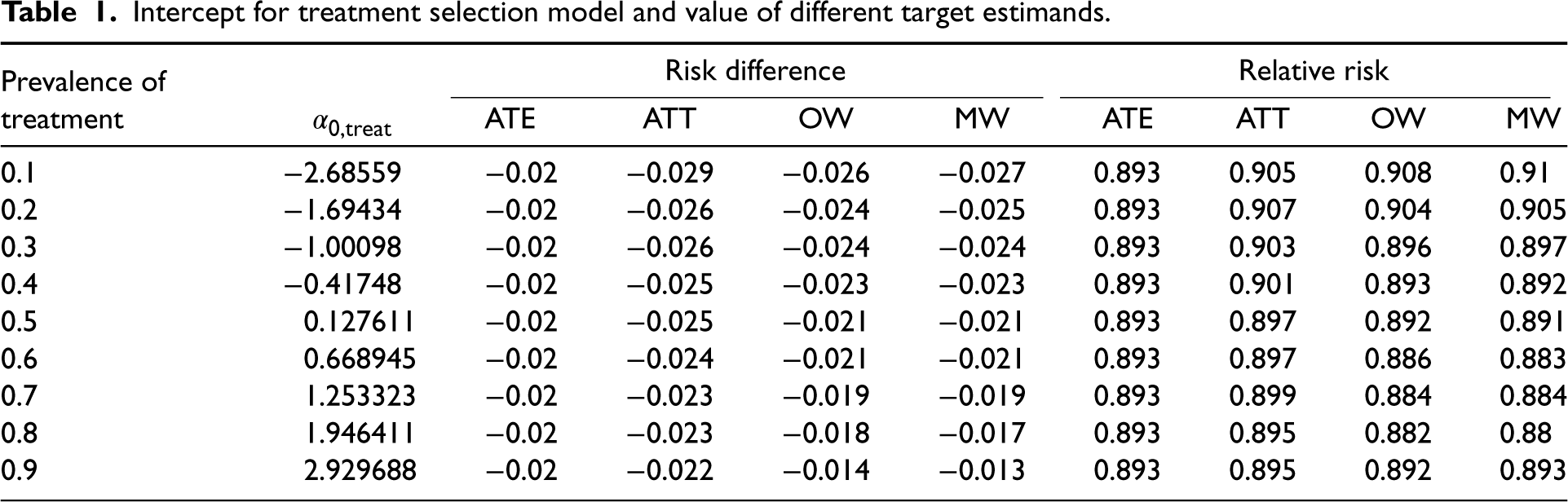
Intercept for treatment selection model and value of different target estimands.
We generated a binary outcome using a logistic model so that the prevalence of the outcome in the super-population was 0.2 if all subjects were untreated and so that the risk difference for treatment was −0.02 with the ATE as the target estimand. The following model was used for simulating binary outcomes:

We drew a random sample of size N from the super-population. In the random sample we estimated the propensity score using a logistic regression model in which treatment status was regressed on the 10 baseline covariates. We estimated four different sets of weights: ATE weights, ATT weights, MW, and OW.2–6 Let 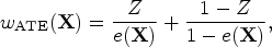
In the random sample of size N we used five methods to estimate the risk difference and its standard error: first, the risk difference was estimated as
We used five methods to estimate the relative risk and the standard error of the log-relative risk. First, the relative risk was estimated as
We constructed 95% confidence using standard normal-theory methods based on the estimated standard error of the estimated treatment effect. We then determined whether the estimated 95% confidence interval contained the true value of the target estimand.
The above methods were repeated using each of the four sets of weights. The above set of analyses was repeated 1000 times. We thus drew 1000 samples, and in each sample we obtained an estimate of the risk difference and the logarithm of the relative risk using each set of weights and each of the methods. We also obtained estimates of the standard error of each estimate and constructed 95% confidence intervals.
Performance measures
We used three performance measures to assess the performance of the different methods for estimating the risk difference and the relative risk: (i) relative bias in the risk difference or log-relative risk; (ii) relative per cent error in the estimated standard error of the risk difference and the log-relative risk; (iii) empirical coverage rates of estimated 95% confidence intervals.
Relative bias was computed as
Relative per cent error in the estimated standard error of the estimated treatment effect was computed as
Empirical coverage rates of estimated 95% confidence intervals were computed as the proportion of estimated confidence intervals that contained the true value of the treatment effect.
Software
The simulations were conducted using the R statistical programming language (version 3.6.3). The weighted analyses were conducted using the PSweight function from the PSweight package (version 1.1.6). In PSweight, the variance of the estimated treatment effect is obtained using the empirical sandwich variance estimator for propensity score weighting estimators based on M-estimation theory. 17 This variance estimator accounts for the uncertainty in estimating the propensity score. The reader is referred elsewhere for further details. 17 Estimation of weighted GLMs using GEE methods was done using the geeglm function in the geepack package (version 1.3-2).
Monte Carlo simulations – results
The binomial-identity GLM and the Poisson-identity GLM resulted in identical estimates of both the risk difference and its standard error across all 1000 iterations of each of the 36 scenarios. For this reason, we only report results for the binomial-identity MSM and not the Poisson-identity MSM when estimating risk differences. Similarly, the binomial-log MSM and the Poisson-log MSM resulted in identical estimates of both the logarithm of the relative risk and its standard error across all 1000 iterations of each of the 36 scenarios. Consequently, we only report results for the binomial-log MSM and not the Poisson-log GLM when estimating relative risks.
Relative bias in estimating risk differences and log-relative risks
For each of the four sets of weights (ATE/ATT/MW/OW), the estimated risk difference or log-relative risk was equal across the different estimation methods within each simulation replicate. Thus, for a given set of weights and measure of effect, the different estimation methods resulted in the same estimated effect. Consequently, the relative bias was equal for the different estimation methods. Results for relative bias are reported in Figure 1. Results for risk differences are reported in the left panel while results for log-relative risks are reported in the right panel. Each panel contains a nested loop plot, with two loops. 25 The outer loop depicts sample size (500, 1000, 5000, and 10,000), while the inner loop depicts prevalence of treatment (0.1 to 0.9 in increments of 0.1). There is one set of lines for each of the four target estimands.
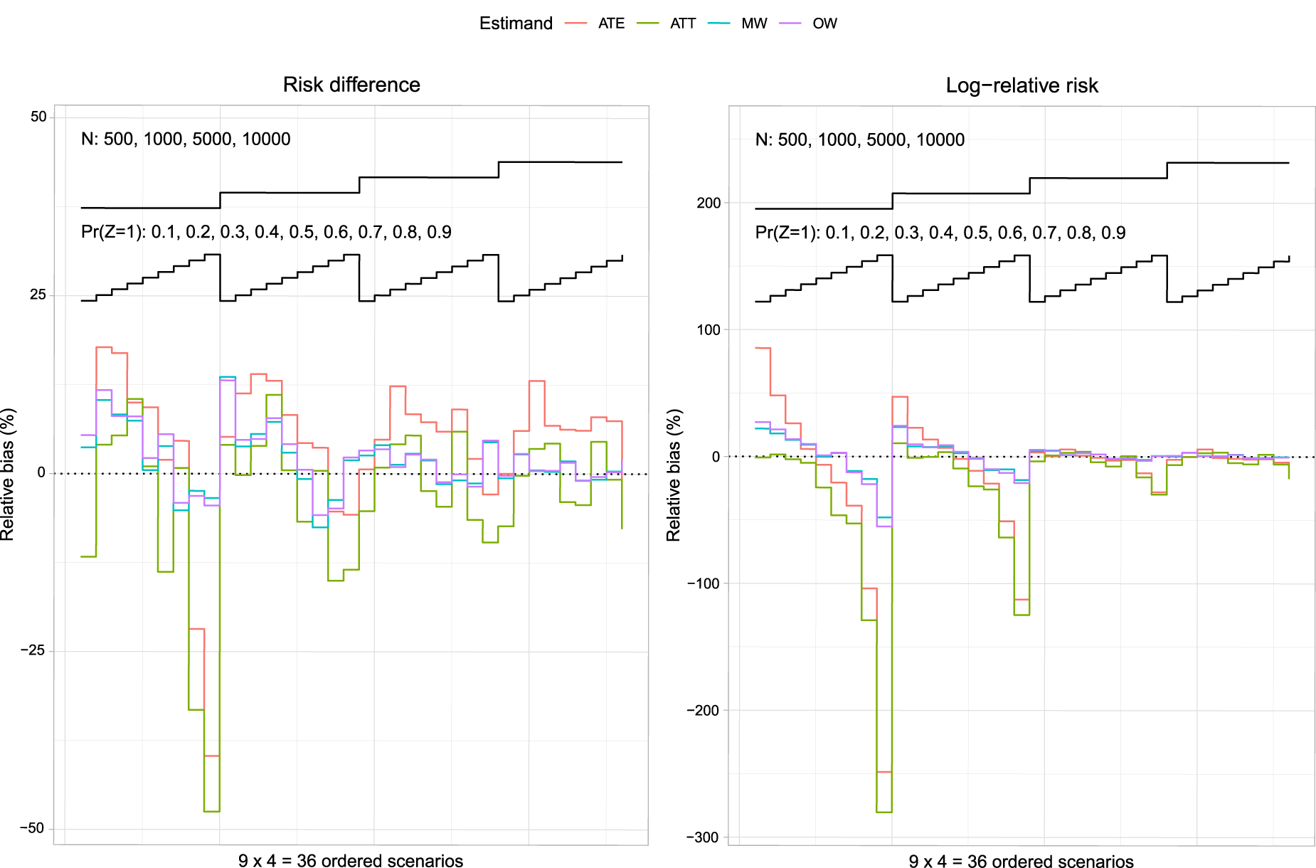
Relative bias (%): risk difference and log-relative risk.
For each target estimand, the magnitude of the relative bias tended to decrease with increasing sample size. Relative bias tended to be the greatest when using ATT weights with a sample size of 500 and a high prevalence of treatment. Note that the relative biases are not intended to be compared between target estimands. For instance, the relative bias when using ATE weights is not comparable to the relative bias when using OW, as the true target estimand for the ATE weights may differ from the true target estimand for the OW (see Table 1 for the values of the different target estimands under different weights).
Relative per cent error in the estimated standard error of the estimated treatment effect is reported in Figure 2 (risk difference) and Figure 3 (log-relative risk). Each figure consists of four panels, one for each of the four target estimands (ATE/ATT/MW/OW). Each panel depicts three nested loop plots, one for each estimation method, with each nested loop plot having two loops. The outer loop depicts sample size (500, 1000, 5000, and 10,000), while the inner loop depicts prevalence of treatment (0.1 to 0.9 in increments of 0.1).
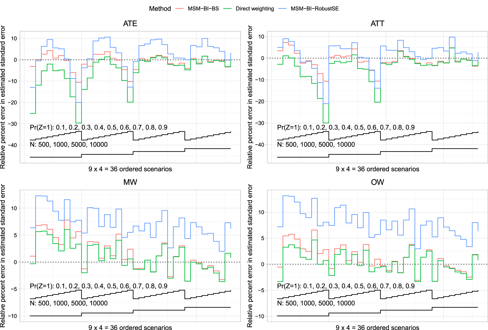
Relative per cent error in the estimated standard error (risk difference).
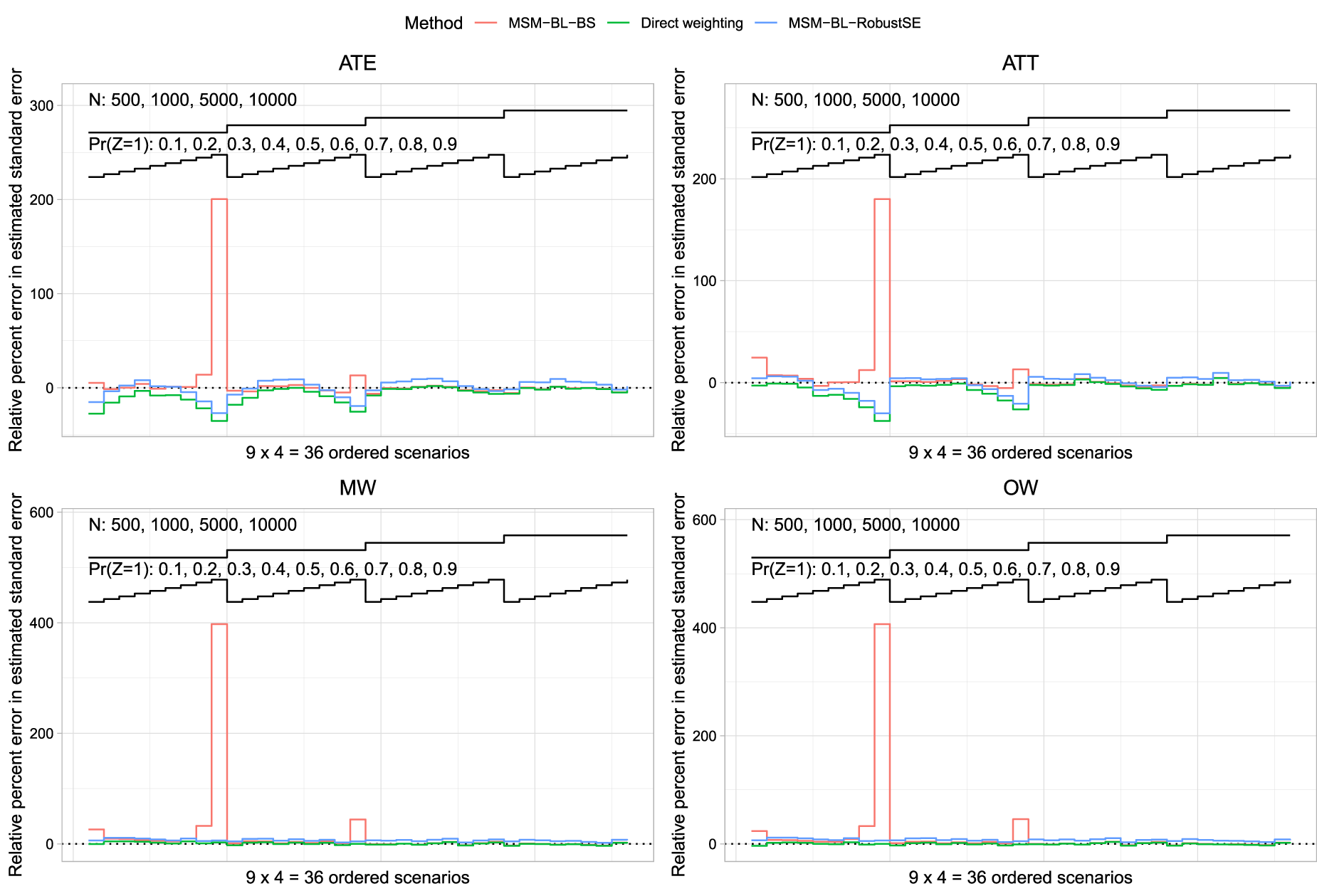
Relative per cent error in the estimated standard error (log-relative risk).
We first discuss results when the risk difference was the measure of effect. When the ATE was the target estimand and the sample size was ≤1000, then MSM-BI-BS tended to produce the most accurate estimates of standard error. When the sample size was 5000 or 10,000, both direct weighting and MSM-BI-BS tended to result in the most accurate estimates of standard error, with minimal differences between the two methods. When the ATT was the target estimand, MSM-BI-BS tended to result in the most accurate estimates of standard error across the different scenarios. When the sample size was ≤1000, all methods tended to underestimate the sampling variability when the prevalence of treatment was high. As with the ATE, when the sample size was 5000 or 10,000, then both direct weighting and MSM-BI-BS tended to result in the most accurate estimates of standard error, with minimal differences between the two methods. When using MW or OW, the use of direct weighting with asymptotic estimates of the standard error tended to result in the most accurate estimates of standard error. However, differences between direct weighting and MSM-BI-BS tended to be minimal. MSM-BI-RobustSE tended to result in the least accurate estimates of standard errors when using MW or OW. In particular, MSM-BI-RobustSE tended to over-estimate the sampling variability of the risk difference when using MW and OW.
We now discuss results when the relative risk was the measure of effect. Across all four sets of weights, when the prevalence of treatment was 0.9 and the sample size was 500, MSM-BL-BS resulted in a large over-estimation of the variance of the sampling distribution of the log-relative risk. Apart from when the prevalence of treatment was 0.9,the use of MSM-BL-BS tended to result in the most accurate estimates of the standard error of the log-relative risk. The large relative error in the estimated standard error when using MSM-BL-BS when the sample size was 500 and the prevalence of treatment was 0.9 makes it difficult to discern differences between the methods in the other scenarios. Figure S1 in the Supplemental Online Material replicates the results from Figure 3, after the exclusion of scenarios in which the prevalence of treatment was 0.9. In scenarios in which the prevalence of treatment was less than 0.9 and the ATE or ATT was the target estimand, none of the three methods had consistently superior performance compared to the other methods. However, the MSM-BL-BS method tended to have good performance. When overlap or MW were used, the direct weighting approach tended to have the best performance of the three methods.
We hypothesize that the large relative error in the estimated standard error for the log-relative risk when using the MSM-BL-BS method with a prevalence of treatment of 0.9 and a sample size of 500 was due to the occurrence of very few outcome events in control subjects in a few of the bootstrap samples. With 500 subjects and a prevalence of treatment of 0.9, there would, on average, be 50 control subjects in each simulated dataset. We simulated outcomes such that the prevalence of the outcome in the super-population was 0.2 if all subjects were untreated. Thus, using a rough approximation, on average, one would anticipate approximately 10 outcome events amongst the 50 controls. The probability of observing three or fewer outcome events would be approximately 0.0057. One would anticipate that, on average, across the 200 bootstrap samples, at least one bootstrap would have three or fewer outcome events in the control subjects, potentially resulting in a very large estimated relative risk with a correspondingly large standard error. In a post-hoc analysis of the simulation results, across the 1000 simulation replicates when using ATE weights, the median standard error of the estimated log-relative risk was 1.00, while the 95th and 99th percentiles were 6.42 and 9.34, respectively. Thus, in a small number of simulation replicates the estimated standard error was very large. Qualitatively similar results were observed for the three other sets of weights.
As noted in Section 3.1, for a given target estimand and measure of effect, each of the methods resulted in the same point estimate across all 1000 iterations of each of the 36 scenarios. Consequently, the empirical standard error (the standard deviation of the estimated measure of effect across the 1000 simulation replicates) was the same for each of the estimation methods. For this reason, we do not compare the empirical standard error across the estimation methods.
Empirical coverage rates are reported in Figure 4 (risk differences) and Figure 5 (log-relative risk). The figures have a structure similar to Figures 2 and 3. Given our use of 1000 simulation replicates, empirical coverage rates that were less than 0.9365 or greater than 0.9635 were statistically significantly different from the advertised rate of 0.95 using a standard normal-theory test. We added horizontal lines denoting empirical coverage rates of 0.9365 and 0.9635 to each of the panels.
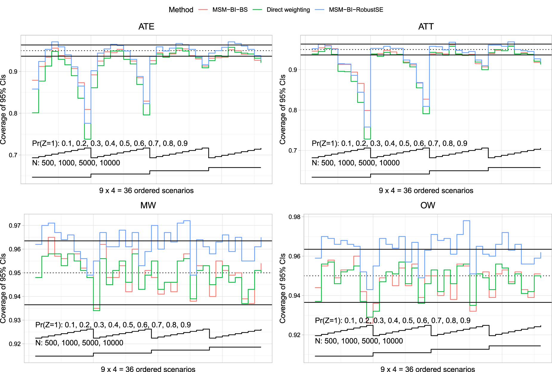
Coverage of 95% confidence intervals (risk difference).
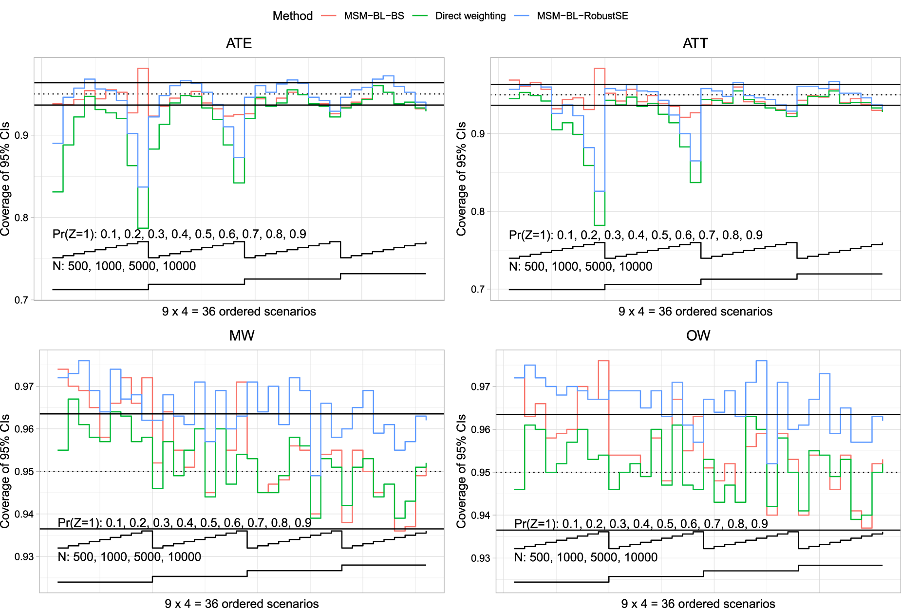
Coverage of 95% confidence intervals (relative risk).
We first discuss results when the risk difference was the measure of effect. When the ATE was the target estimand, all methods tended to result in confidence intervals with lower than advertised coverage rates when the prevalence of treatment was either low or high. The magnitude of the divergence from the advertised coverage rates decreased with increasing sample size. When the prevalence of treatment was close to 0.5, MSM-BI-BS tended to result in confidence intervals whose empirical coverage rates were closest to the advertised rate. When the ATT was the target estimand, all methods tended to result in confidence intervals whose coverage rate was lower than advertised when the prevalence of treatment was high. As with the ATE, the magnitude of divergence from the advertised rate decreased with increasing sample size. When using MW or OW, both direct weighting and MSM-BI-BS tended to produce confidence intervals whose empirical coverage rates did not differ from the advertised rate. In contrast to this, MSM-BI-RobustSE often produced confidence intervals whose empirical coverage rates were conservative.
We now discuss results when the relative risk was the measure of effect. When the ATE was the target estimand, both direct weighting and MSM-BL-RobustSE produced confidence intervals whose empirical coverage rates were lower than advertised when the sample size was ≤1000 and the prevalence of treatment was low or high. In contrast to this, in most scenarios MLM-BL-BS produced confidence intervals whose empirical coverage rates were not different from the advertised rate. When the ATT was the target estimand, both direct weighting and MSM-BL-RobustSE tended to produce confidence intervals whose empirical coverage rates were lower than the advertised rate when the prevalence of treatment was high. The magnitude of divergence from the advertised rate decreased with increasing sample size. When using MW and OW, all methods tended to produce confidence intervals whose empirical coverage rates were at least 0.9365. In many scenarios, MLM-BL-RobustSE tended to produce confidence intervals whose empirical coverage rates were conservative.
As noted above, the use of the Poisson-identity GLM produced estimates identical to the binomial-identity GLM in each of the simulation replicates, while the use of the Poisson-log GLM produced estimates identical to the binomial-log GLM. However, for the sake of completeness, results for the Poisson-based MSMs are reported in Figures S2 to S5 in the Supplemental Online Material.
We provide a case study to compare the use of different methods for estimating the risk difference and the relative risk. The case study consisted of patients discharged from hospital with a diagnosis of AMI. The exposure was receipt of a prescription for a beta-blocker at hospital discharge. The binary outcome was death within one year of hospital discharge.
Methods
We used a subset of data from a previously-published study, consisting of 6984 patients who were discharged alive from hospital with a diagnosis of AMI in Ontario, Canada, between 1 April 1999 and 31 March 200126,27 and who were eligible for beta-blocker therapy at hospital discharge. Baseline information was available on patient demographics, presenting signs and symptoms, classic cardiac risk factors, comorbid conditions and vascular history, vital signs on admission, and results of laboratory tests. The exposure of interest was whether the patient was prescribed a beta-blocker at hospital discharge. Seventy-two per cent of subjects were prescribed a beta-blocker at hospital discharge. The outcome was a binary outcome denoting whether the patient died within one year of hospital discharge. Twelve per cent of subjects died within one year of hospital discharge. The propensity score was estimated using a logistic regression model in which receipt of a beta-blocker at hospital discharge was regressed on 34 baseline covariates.
The statistical methods described above for estimating the risk differences and relative risks along with their associated 95% confidence were used. We did not use the MSM based on a Poisson-identity GLM for estimating risk differences, as it produced identical results to the binomial-identity GLM. Similarly, we did not use the MSM based on a Poisson-log GLM for estimating relative risks, as it produced identical results to the binomial-log GLM.
Results
The estimated risk differences and their associated 95% confidence intervals are reported in the left panel of Figure 6, while the estimated logarithms of the relative risk and their associated 95% confidence intervals are reported in the right panel of Figure 6. Each panel is a forest plot with one horizontal bar for each combination of estimands and method. For a given combination of estimand (ATE/ATT/MW/OW) and measure of effect (risk difference or log-relative risk), the point estimate was identical across estimation methods. When estimating confidence intervals for the risk difference, the ratio of length of the widest confidence interval to the narrowest confidence interval ranged from 1.20 to 1.23 across the four sets of weights. When estimating confidence intervals for the log-relative risk, these ratios ranged from 1.19 to 1.23 across the four sets of weights. For a given set of weights, the use of the MSM with a bootstrap variance estimator resulted in the narrowest 95% confidence intervals, while the use of the MSM with the robust variance estimator resulted in the widest 95% confidence intervals. Despite these differences, in examining Figure 6, for a given target estimand and measure of treatment effect, one would draw qualitatively similar conclusions regardless of which estimation method was used.
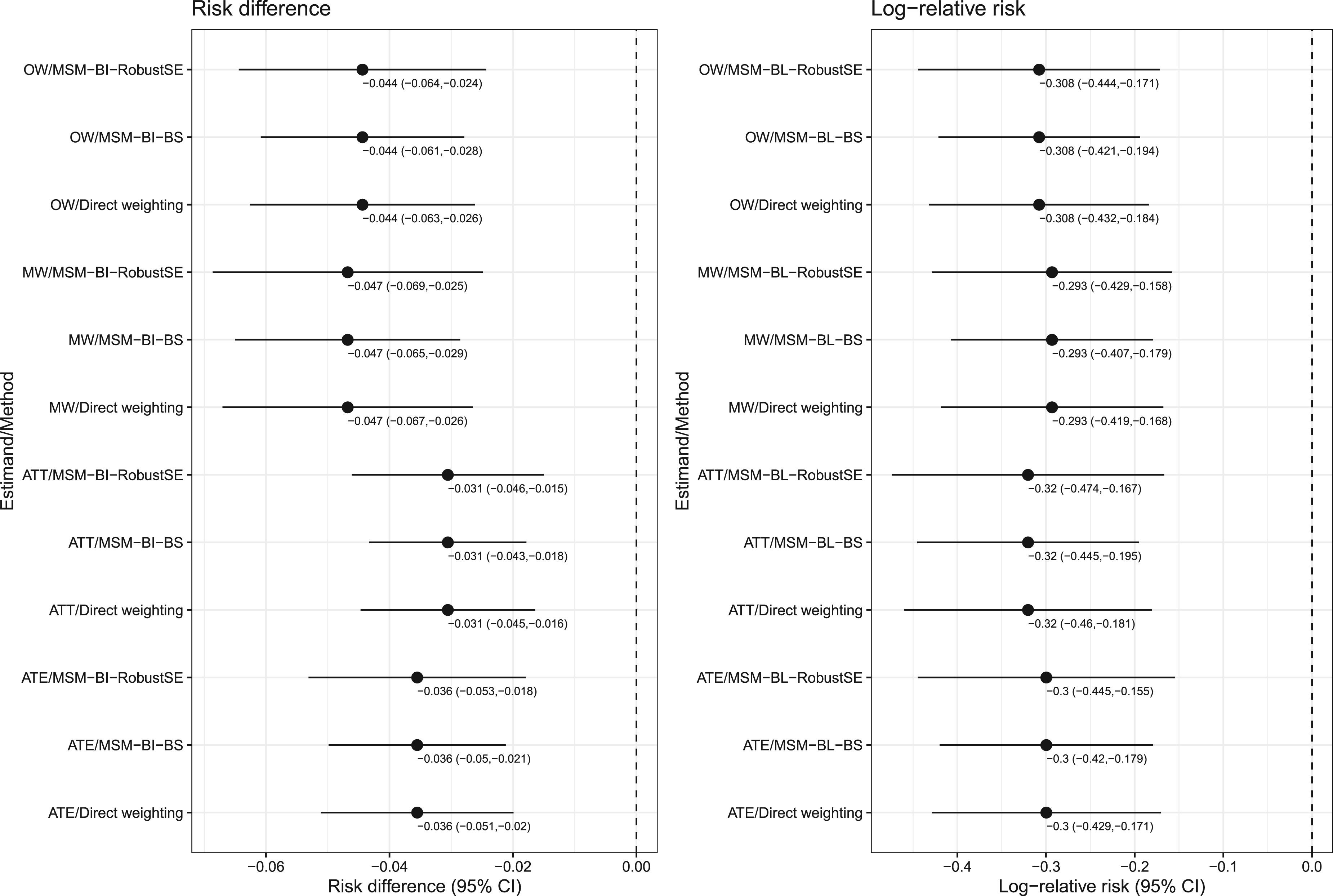
Case study: estimates of risk difference and log-relative risk.
We assessed the performance of MSMs based on weighted univariate GLMs for estimating risk differences and relative risks. We compared the conventional robust variance estimator for a GLM estimated using GEE methods with an independence working correlation matrix with the use of the bootstrap for estimating the standard error of risk differences and the log-relative risk. These methods were compared with the use of direct weighted estimators with asymptotic variance estimators. We summarize our findings as follows. First, both direct weighting and MSMs resulted in identical point estimates of the risk difference or relative risk. Consequently, all methods had the same empirical standard deviation. Thus, the difference between the methods was the degree to which the estimated standard errors approximated the standard deviation of sampling distribution of the risk difference or the log-relative risk. Second, when using ATE or ATT weights and the sample size was ≤1000, then an MSM with the bootstrap variance estimator tended to result in the most accurate estimates of the standard error. When the sample size was >1000, then the direct weighting approach with asymptotic estimates of the standard error and the MSM with a bootstrap variance estimator tended to have comparable performance. Third, when using OW or MW, the direct weighting approach and the MSM with the bootstrap variance estimator tended to have comparable performance. Based on differences between these two methods when estimating the relative risk and both the sample size was small and the prevalence of treatment was very high, we would recommend the use of the direct weighting estimator. Fourth, in general, the MSM with a robust variance estimator had worse performance than did the MSM with the bootstrap variance estimator. Consequently, when using an MSM, we would recommend that the bootstrap variance be used, particularly if the prevalence of treatment is not close to one. Fifth, when using a univariate MSM, identical estimates of both the risk difference or the log-relative risk and its associated standard error obtained when using either the binomial distribution or the Poisson distribution. Thus, in applied studies, either of these distributions can be used.
The robust variance estimator with conventional ATE weights or OW is known to be conservative. Despite this, the robust variance estimator, rather than the direct weighting method, is often used by many applied investigators. We hypothesize that this is because the robust variance estimator can be implemented easily using standard statistical software (e.g. using standard procedures or functions in R, SAS or Stata). In contrast to this, the use of the appropriate asymptotic variance estimator for the direct weighted estimator often requires that a specialized package be used (e.g. the PSweight package in R). Similarly, the use of the bootstrap variance estimator with weighted GLMs may require more complex programming by the analyst.
Only a few studies have examined the performance of a robust variance estimator when using weighted regression models to estimate causal effects. An earlier study examined methods based on the propensity score to estimate marginal hazard ratios. 28 Weighted Cox models resulted in estimates of the marginal hazard with minimal bias when either the ATE or the ATT was the target estimand. The use of a robust variance estimator with ATE weights tended to under-estimate the standard deviation of the log-hazard ratio by between approximately 0% and 10% depending on the true marginal hazard ratio. However, the use of a robust variance estimator with ATT weights tended to over-estimate the standard deviation of the log-hazard ratio by between approximately 30% and 45% depending on the true marginal hazard ratio. In a subsequent article, the author showed that the use of the bootstrap with weighted Cox models resulted in accurate estimation of the standard error of log-hazard ratios when either the ATE or the ATT was the target estimand. 29 Arona Diop and colleagues stated that the robust variance estimator used with OW is conservative. 30 Reifeis and Hudgens examined the performance of the robust variance estimator when used with ATT weights and found that the estimator may be either conservative or anticonservative, concluding that the resultant confidence intervals will not be valid. 31 We are unaware of the previous similar results for MW.
Only a few studies have examined the performance of propensity score methods for estimating risk differences and relative risks. The current study restricted its focus on the use of propensity score weighting to estimate risk differences and relative risks. A study from 2008 compared the performance of matching on the propensity score, stratification on the quintiles of the propensity score, and covariate adjustment using the propensity score (but not propensity score weighting) to estimate relative risks. 32 Propensity score matching and stratification on the quintiles of the propensity score resulted in estimates of relative risk with similar mean squared error (MSE), with matching producing estimates with less bias and stratification producing estimates with greater precision. A study from 2010 compared the performance of different propensity score methods for estimating risk differences. 33 Estimators based on inverse probability of treatment weighting (IPTW) had lower MSE compared to other propensity score methods, while a doubly robust version of IPTW had superior performance compared to the other methods. A 2010 study examined the performance of weighted binomial-identity MSMs for estimating risk differences. 34 Using simulations, the authors showed that the absolute bias tended to be minimal. However, empirical coverage rates had lower than advertised coverage rates when confounding was strong. There were four primary differences between their simulations and those in the current study. First, their simulation design only included two confounding variables, whereas the design in the current study had 10 confounding variables, which is more representative of settings in which propensity score methods are used. Second, while they restricted their focus on the robust variance estimator, the current study also considered the use of the bootstrap. We found that in several settings, the use of the bootstrap resulted in improved inferences compared to the use of the robust variance estimator. Third, the earlier study restricted attention to the risk difference, while we focused on estimation of both the risk difference and the relative risk. Fourth, the earlier study focused only on estimation using the MSM approach, whereas we compared the use of MSMs with direct weighting. A 2011 study compared the use of paired versus unpaired analyses when making inferences about risk differences when using propensity score matching. 35 It was shown that the use of paired analyses (e.g. the use of McNemar's test) was superior to that of unpaired analyses (e.g. the use of the standard Chi-squared test). A 2017 study compared the performance of full matching on the propensity score with that of nearest neighbour matching (NNM) and IPTW for estimating risk differences and relative risks. 36 All methods worked well when the strength of confounding was relatively weak. With stronger confounding, NNM with a caliper had good performance across a range of scenarios. A study from 2017 described how NNM on the propensity score can be combined with covariate adjustment using the propensity score (so called double propensity score adjustment) to make inferences about risk differences. 37
There are certain limitations to the current study. The primary limitation relates to our use of Monte Carlo simulations. Due to the computational intensity of using Monte Carlo simulations to examine the performance of bootstrap methods, we were only able to examine a limited number of scenarios. However, we examined 36 different scenarios characterized by different combinations of sample size and prevalence of treatment. These scenarios reflect many of the settings in which propensity score methods are applied in clinical and epidemiological research. When using direct weighting we only examined the use of an asymptotic variance estimator and did not consider bootstrapping. The rationale for that limitation was that we had examined the performance of the bootstrap with direct weighting in a recent study. 18 In that prior study we found that when the ATE was the target estimand and sample sizes were ≤1000, that the bootstrap resulted in more accurate estimates of standard errors than the asymptotic variance estimator. Similarly, when the ATT was the target estimand and both sample sizes were ≤1000 and the prevalence of treatment was moderate to high, then the bootstrap produced estimates of standard errors that were more accurate than the asymptotic variance estimators. When using MW and OW, both the asymptotic variance estimator and the bootstrap resulted in accurate estimates of standard errors. Another limitation relates to our restriction to the use of univariate GLMs and we did not consider adjustment for additional covariates. While we observed that the use of binomial distribution and a Poisson distribution resulted in identical results, we do not anticipate that this would necessarily be true if using multivariable GLMs. The results of the current study should not be extrapolated to analyses in which GLMs are adjusted for a set of baseline covariates in addition to the binary treatment variable. Another limitation is that we only used parametric regression models to estimate the propensity score from which the weights were derived. Further research is required to examine whether our conclusions persist when machine learning algorithms are used to estimate the propensity score.
We compared the performance of variance estimators for two target estimands (risk differences and relative risks) and four sets of weights (ATE weights, ATT weights, OW, and MW). Our intent was not that results be compared between different sets of weights. In general, in applied research, analysts should select the set of weights that best addresses the study question. The different sets of weights should not be seen as interchangeable. 7 The results of the current study should be used to guide the analyst in the choice of variance estimation method once a specific set of weights has been selected.
In the current paper we restricted our attention to weighting-based methods for estimating risk differences and relative risks. Regression-based methods, also known as G-computation, can be used to estimate risk differences and relative risks.38–40 Cheung described a modified least-squares regression approach to estimating the risk difference. 41 The current study restricted its focus on the use of propensity score weighting to estimate risk differences and relative risks.
In summary, both a direct weighting approach and MSMs based on weighted univariate GLMs resulted in the identical estimates of risk differences and relative risks. When sample sizes were small to moderate, the use of an MSM with a bootstrap variance estimator tended to result in the most accurate estimates of standard errors. When sample sizes were large, the direct weighting approach and an MSM with a bootstrap variance estimator tended to produce estimates of standard error with similar accuracy. Finally, when using a MSM to estimate risk differences and relative risks, it is, in general, preferable to use a bootstrap variance estimator than the robust variance estimator.
Supplemental Material
sj-pdf-1-smm-10.1177_09622802241247742 - Supplemental material for The performance of marginal structural models for estimating risk differences and relative risks using weighted univariate generalized linear models
Supplemental material, sj-pdf-1-smm-10.1177_09622802241247742 for The performance of marginal structural models for estimating risk differences and relative risks using weighted univariate generalized linear models by Peter C Austin in Statistical Methods in Medical Research
Footnotes
Acknowledgements
This study was supported by ICES, which is funded by an annual grant from the Ontario Ministry of Health (MOH) and the Ministry of Long-Term Care (MLTC). This study also received funding from: the Canadian Institutes of Health Research (CIHR) (PJT 183902). This document used data adapted from the Statistics Canada Postal CodeOM Conversion File, which is based on data licensed from Canada Post Corporation, and/or data adapted from the Ontario Ministry of Health Postal Code Conversion File, which contains data copied under license from ©Canada Post Corporation and Statistics Canada. Parts of this material are based on data and/or information compiled and provided by: CIHI and the Ontario Ministry of Health. The analyses, conclusions, opinions and statements expressed herein are solely those of the authors and do not reflect those of the funding or data sources; no endorsement is intended or should be inferred. As a prescribed entity under Ontario's privacy legislation, ICES is authorized to collect and use health care data for the purposes of health system analysis, evaluation and decision support. Secure access to these data is governed by policies and procedures that are approved by the Information and Privacy Commissioner of Ontario. The dataset from this study is held securely in coded form at ICES. While legal data sharing agreements between ICES and data providers (e.g. healthcare organizations and government) prohibit ICES from making the dataset publicly available, access may be granted to those who meet pre-specified criteria for confidential access, available at ![]() (email: das@ices.on.ca). The use of data in this project was authorized under section 45 of Ontario's Personal Health Information Protection Act, which does not require review by a research ethics board. The opinions, results and conclusions reported in this paper are those of the authors and are independent from the funding sources.
(email: das@ices.on.ca). The use of data in this project was authorized under section 45 of Ontario's Personal Health Information Protection Act, which does not require review by a research ethics board. The opinions, results and conclusions reported in this paper are those of the authors and are independent from the funding sources.
Declaration of conflicting interests
The author declared no potential conflicts of interest with respect to the research, authorship, and/or publication of this article.
Funding
The author disclosed receipt of the following financial support for the research, authorship, and/or publication of this article: This work was supported by the Canadian Institutes of Health Research (CIHR) (grant number PJT 183902).
Supplemental material
Supplemental material for this article is available online.
References
Supplementary Material
Please find the following supplemental material available below.
For Open Access articles published under a Creative Commons License, all supplemental material carries the same license as the article it is associated with.
For non-Open Access articles published, all supplemental material carries a non-exclusive license, and permission requests for re-use of supplemental material or any part of supplemental material shall be sent directly to the copyright owner as specified in the copyright notice associated with the article.