Sage Journals: Discover world-class research

Abstract

We explore the impact of the COVID-19 shock on a very high frequency indicator: the Spanish daily sales data compiled by the Tax Agency. Firstly, we present a detailed list of the issues related to its modeling, its decomposition (trend, seasonality, and irregularity) and its final seasonal adjustment, which requires a set of deterministic factors linked mostly to calendar effects. Then, we assess the impact of the COVID-19 shock on these tasks. This assessment provides a timely perspective on the evolution of the shock and the challenges that it posed for modeling and seasonal adjustment, clearly related to its unusual and extreme features. The aim of the paper is eminently empirical and dominated by the need to square the unprecedented shock with the available methods and software in a computing environment centered on the R programming language. The methodology draws heavily on a structural approach and it is currently in use by the Tax Agency to compile and disseminate its daily sales data.

Keywords

tax data very high frequency time series deterministic effects calendar effects unobserved components model

1. Introduction

The year 2020 will be marked in the future books of History as one of the most outlying and tragic ones, due to the spread of the SARS-CoV-2 virus (CV19 for brevity) and the resulting health and economic crises linked to the policy interventions enforced by governments around the world aimed at containing and mitigating the disease. Both crises were global, sharp, and very intense, without historical precedents and posing serious and numerous challenges for many activities, ranging from health surveillance and prevention to economic policy and crisis management. Of course, one of the most affected activities has been economic measurement and monitoring, fostering a plethora of proposals and methods to compensate the informational gaps and the modeling difficulties created by the crisis (Leiva-León et al. 2020; Lenza and Primiceri 2020; Maroz et al. 2021; Ng 2021; Primiceri and Tambalotti 2020; Schorfheide and Song 2020).

The CV19 shock can be considered as an exogenous shock linked to adverse health conditions with sharp and huge economic consequences. Although its origin is clearly exogenous, many policy decisions oriented toward its control and containment (lockdowns, mobility constraints, capacity limits, etc.) were critical to shape its economic effects. In this way, we will consider two separate phases: lockdown and new-normal (also called “recovery” or “de-escalation”).

This paper contributes along two different lines. The first one is to present a statistical indicator that retains the “hard” nature of the core of the official short-term indicators but with a sampling frequency (daily) very well suited for the analysis of shocks like the CV19 one: the daily sales compiled by the Spanish Tax Agency as a by-product of its on-line Value Added Tax (VAT) system.

One important and valuable feature of sales data is its “hard” nature. Unlike most alternative sources whose use has increased due to the shock (Ten et al. 2022), sales data define a complete valuation at current prices of effective transactions, measured directly from administrative records. This fact allows its easy integration with the rest of official statistical sources, especially those related to the National Accounts and to standard economic indicators like the retail sales or the index of industrial production.

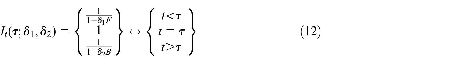
The second line is methodological: how to deal with the impact of the CV19 shock on the econometric models used to represent and seasonally adjust daily economic data. As we will explain later in detail, our proposal is based on an intervention analysis especially designed to cope with the bulk of the impact of the CV19 shock on the level of the daily sales data. This approach may be considered as an adaptation of the official recommendations related to the seasonal adjustment of monthly indicators affected by the CV19 shock to the daily case (Eurostat 2020). These recommendations hinge around expanding the models used for seasonal adjustment, in order to include an intervention analysis to take into account the effects of the CV19 shock.

At the time of writing this paper (August 2022) it is unavoidable to have a hindsight perspective about the CV19 shock that permeates the analysis, although we have tried to keep the real-time perspective in mind as much as possible.

The paper is organized as follows. The second section presents the data. The third section develops the econometric methodology, which is implemented in two stages: preprocessing and decomposition (signal extraction). The empirical results are presented in the fourth section, with the focus on the estimation of the CV19 shock across several specifications. The paper ends presenting the main conclusions and future developments.

2. Data

Daily sales series of monthly VAT taxpayers comes from the Immediate Supply of Information System (SII, Sistema Inmediato de Información), introduced in January 2017 and officially implemented by the Spanish Tax Agency since July 2017 (Cuevas et al. 2021; Tax Agency 2017).

This system allows the exchange of tax information between the Spanish Tax Agency and taxpayers required by the SII practically in real time, by supplying the detail of the invoicing records within four days, through the electronic platform of the Spanish Tax Agency.

In this way, both tax management and tax compliance are improved (e.g., by the taxpayers comparison of the information in their books with the information provided by their customers and suppliers).

The group compulsorily included in the SII is made up of all those taxpayers whose obligation to declare VAT is monthly:

Large Companies (turnover greater than 6,010,214.04 EURO in the previous year). This very specific cut-off is just a legal threshold, not a statistical one.

Those companies that pay taxes through the special regime for groups of companies. A group of companies is considered when it is formed by a parent company and its subsidiaries. They must be firmly bound to one another.

Registered, voluntarily, in the Monthly VAT Return Registry.

In addition, this system is applied to those taxpayers who voluntarily adopt it.

Thus, the SII comprises about 63,000 taxpayers representing around 70% of the country’s total business turnover, with a great diversity of coverage by activities.

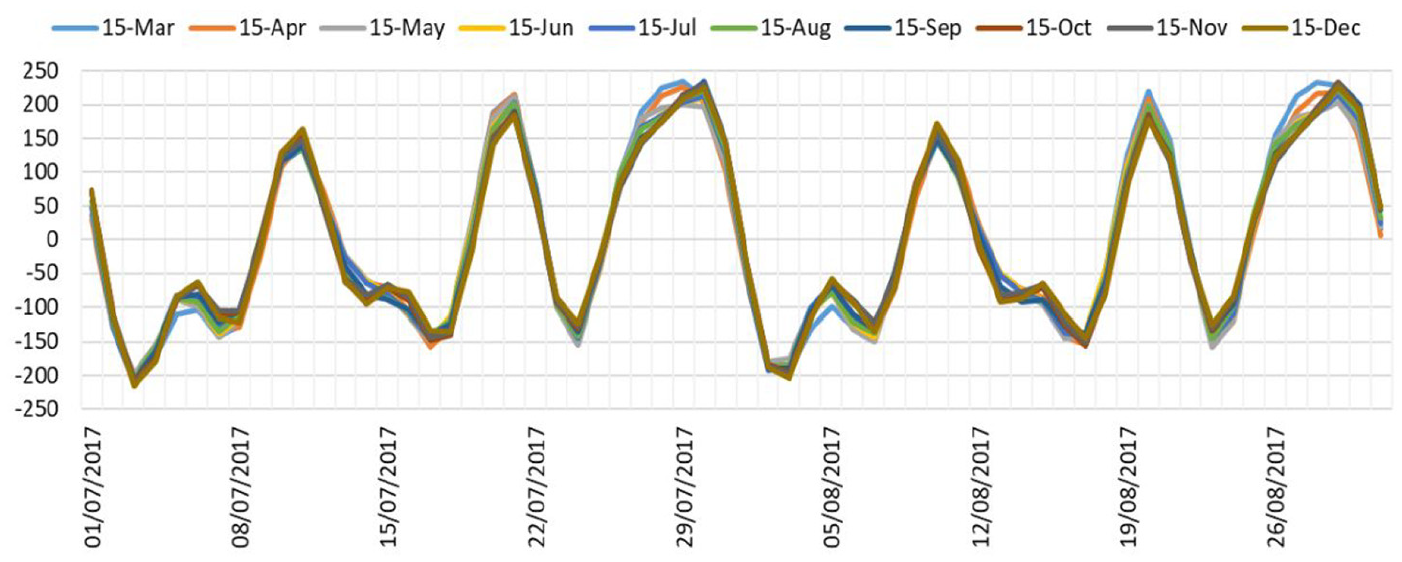
Figure 1a to c show the daily time series with different samples and Figure 1d shows the corresponding monthly average, in order to be able to appreciate the main characteristics of the series. The sample considered comprises from the full-fledged implementation of the SII (July 1st, 2017) until the end of 2020. At first glance, it is possible to see the large volatility of the series, due to the different invoicing patterns, that we will comment on later, such as the large effect of the end of the month, which makes very difficult to distinguish a relevant signal of the underlying evolution. Likewise, a clear weekly pattern can also be observed, as well as a significant annual seasonality.

Figure 1.

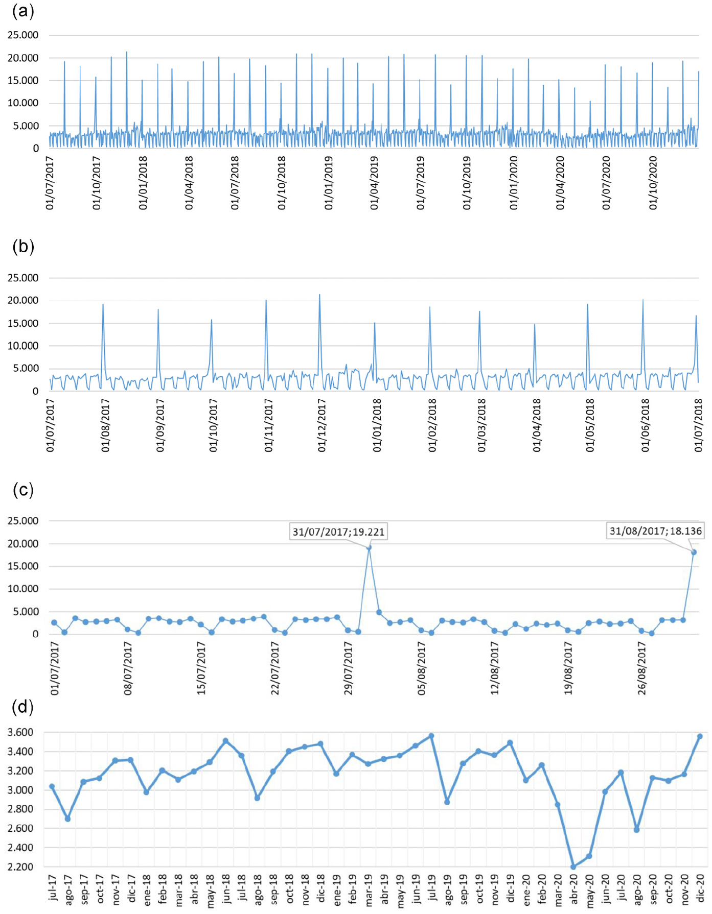
(a) Daily sales from SII (million EURO). Sample 01/07/2017 to 31/12/2020. (b) Daily sales from SII (million EURO). Sample 01/07/2017 to 01/07/2018. (c) Daily sales from SII (million EURO). Sample 01/07/2017 to 31/08/2017. (d) Daily sales from SII (million EURO). Monthly averages.

We have used temporal averaging in Figure 1d as a rough and simple way to discount the weekly and the monthly seasonality, making thus visible a trend and an annual seasonal pattern, both somehow distorted by the CV19 shock.

As a general rule, firms must send their invoices to the Tax Agency four days after they have been issued. However, the information received by the Tax Agency is not always the final one, as it can be completed and corrected in the following days. Experience indicates that it is necessary to wait around two weeks for the stabilization of the levels that allows us to consider the data as definitive.

3. Modeling Daily Data

In this section, we present the econometric methodology used in the paper. Modeling economic daily time series poses several and difficult challenges due to the coexistence of multiple seasonal components linked to various frequencies, the strength of its irregular component and its sensitivity to exogenous factors (e.g., outliers) that distort its usual behavior and, last but not least, the complex structure of the calendar: different length and composition of the months, moving festivities (e.g., Easter), leap years, and a time-varying calendar of working days that interacts with the composition of the months (Ladiray et al. 2018).

We use the structural model of unobserved components proposed by De Livera et al. (2011) to perform modeling and seasonal adjustment of the Spanish daily sales data. The model, called TBATS (acronym for Trigonometric seasonality, Box-Cox transformation, ARMA innovations, Trend, and Seasonality), complemented with a suitable dynamic-regression pre-processing, provides a flexible although parsimonious way to handle the complex nature of daily time series. The econometric methodology has two steps:

Pre-processing (linearization). In this step we apply an intervention analysis by means of exogenous deterministic variables designed to control for the presence of outliers and specific calendar effects that, due to their moving nature, do not fit well into the structural representation considered by TBATS (Bell and Hillmer 1983; Hillmer et al. 1983). This intervention analysis is a preprocessing step of the observed series that renders it suitable for TBATS.

Structural decomposition using TBATS. The pre-processed time series is decomposed into trend-cycle, seasonality, and irregularity. As we will expose below, the seasonal component has a complex nature due the coexistence of multiple seasonal patterns, some of them with fractional periodicities.

Let us now explain both steps with some detail.

3.1. Pre-Processing (Linearization)

Although TBATS can handle fractional seasonal periodicities (e.g., 30.4375 days for the monthly seasonality) the fact that this fractional feature is due to a (weighted) average of different periodicities (28, 29, 30, and 31 days) and not to a fixed periodical pattern hampers its modeling, especially when the time span is not large, as is our case. Easter and bank holidays share this complex periodicity but on an annual basis. This explains why De Livera et al. (2011) strongly recommend the use of a pre-preprocessing step before applying TBATS.

In addition, the monthly seasonal pattern is heavily concentrated on some specific days of the month (e.g., first day, last day, etc.), diverging from the smooth profile that characterizes the trigonometric functions used by TBATS. This is why Hyndman (2017) recommends a deterministic specification for the monthly seasonality.

All these effects are represented by deterministic variables and their impact on the observed time series is estimated using a regression model that includes a linear trend and a multiple seasonal component affine to the one used in the trigonometric seasonal representation used by TBATS. The regression model is:

y_{t} = η x_{t} + λ_{0} + λ_{1} t + \sum_{i = 1}^{3} \sum_{j = 1}^{k_{i}} [ρ_{j}^{(i)} \sin (\frac{2 j π t}{m_{i}}) + φ_{j}^{(i)} \cos (\frac{2 j π t}{m_{i}})] + ε_{t}

(1)

Being:

y _t: (log-transformed) observed variable (daily sales).

x_t: m deterministic (dummy) variables linked to the bank holidays and to a set of within-the-month effects that are described at length in section 4.1. The vector of parameters $η$ measures its impact on the level of the daily sales.

The term $λ_{0} + λ_{1} t$ represents a linear trend, being $t = 1 . . T$ the time index.

The index $i = 1 . . 3$ represents the seasonal components (weekly, monthly, and annual) and the index $j = 1 . . k_{i}$ represents the harmonics that define each seasonal component.

Each seasonal component is defined by its periodicity m_i (in days). Based on a previous analysis (Cuevas et al. 2021) we have considered three components (weekly, monthly, and yearly) whose periodicities, expressed in days, are: 7, 30.4375, and 365.25. The periodicity of the monthly seasonal component takes into account both the different length of the months and the leap years. The fractional periodicity of the annual seasonality is only due to the presence of leap years (Ladiray et al. 2018).

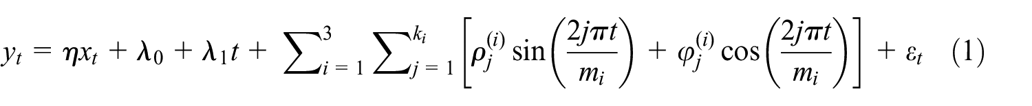
The parameters $ρ_{j}^{(i)}$ and $φ_{j}^{(i)}$ represent, for the i-th seasonal component, the impact of the j-th trigonometric term (sine or cosine, respectively) on the observed time series.

$ε_{t}$ : Gaussian error term.

The decision to take logarithms is based on a mean-range analysis performed on the pre-CV19 sample (up to March 15, 2020). This analysis splits this sample into a set on non-overlapping subsamples of 31 days, computing for each one the range (difference between its maximum and minimum) and its mean. The length of the subsamples (31 days) covers at the same time weekly and monthly fluctuations. We have trimmed each subsample by excluding its maximum and minimum values, in order to reduce the influence of the outliers on the means and ranges. The corresponding scatterplot of the trimmed subsamples can be seen in Figure 2.

Figure 2.

Mean-range analysis of the pre-CV19 sample.

There is a clear tendency of higher mean levels to be associated with higher volatility. This association may be stabilized by applying logarithms. The slope of the underlying regression line is statistically different from zero.

A preliminary TBATS estimate of the Box-Cox parameter using the pre-CV19 sample yields a value of 0.8387, suggesting the convenience to apply some stabilizing transformation to the data and moving us to apply the logarithmic transformation in all the cases.

It is interesting to note that the regression model Equation (1) can be considered as a one-equation approximation to the complete structural TBATS model that will be presented below, especially due to its similar treatment of the (multiple) seasonality. This similitude enhances the complementarity of steps 1 and 2.

The number of harmonics, k_i, associated with each seasonal component (weekly, monthly, and annual) can be determined by means of a preliminary estimate of the TBATS model applied to the original time series.

Equation (1) is estimated by Ordinary Least Squares (OLS) and allows us to linearize the observed time series by subtracting the estimated effect due to the m deterministic variables linked to the bank holidays and to a set of within-the-month effects, x_t:

z_{t} = y_{t} - η x_{t}

(2)

This correction does not consider the remaining deterministic variables (the linear trend and the trigonometric seasonals) that are thus just proxy variables introduced to reduce the danger of obtaining biased estimates for the dummy effects collected in $η$ .

3.2. Structural (TBATS) Decomposition

The TBATS approach is based on the representation of the unobserved components (trend, seasonality, irregularity) by means of explicit dynamic models (Harvey 1989). An alternative approach, based on reduced-form models, offers great flexibility to include exogenous variables but does not provide an estimate of the underlying components (Espasa et al. 1996; Liu 2005). Although less complete, we have also used this approach as a cross-check (Cuevas et al. 2019).

Following the structural approach, the model incorporates a parsimonious but rather general representation of the trend. It also includes an explicit model for the irregular component that acts as a sort of “safety valve,” accommodating elements that, for whatever reason, did not find a proper fit within the basic systematic components (trend and seasonality). In this way, the plain representation of these two components does not compromise neither the fit of the model to the sample nor its forecasting performance.

The general TBATS model assumes that the linearized time series (z_t) results from the aggregation of three unobserved components: trend (p_t), seasonality (s_t), and a stationary innovation (u_t):

z_{t} = p_{t} + s_{t} + u_{t}

(3)

The innovation u_t plays an additional role as the stochastic input for the other two components. In this way, both the trend and the seasonality depend on a single shock that, properly scaled and filtered, generates them. In general, we assume that u_t evolves according to a stationary and invertible autoregressive and moving average (ARMA) model:

(1 - ϕ_{1} B - \dots - ϕ_{p} B^{p}) u_{t} = (1 - θ_{1} B - \dots - θ_{q} B^{q}) e_{t}

(4)

The ultimate shock e_t is a Gaussian white noise with zero mean and fixed variance $σ^{2}$ :

e_{t} ~ iid N (0, σ^{2})

(5)

An interesting feature of TBATS is that it can handle complex seasonal patterns, comprising both multiple periodicities (weekly, monthly, and yearly) and fractional periodicities (e.g., 30.4375 days for monthly seasonality or 365.25 for annual seasonality).

This complex seasonal pattern is one of the most important differences between a daily time series and its monthly/quarterly counterpart. In the latter case, the seasonal component is unique and of integer periodicity (twelve months and four quarters, respectively). Of course, this additional complexity requires an additional layer of specific modeling.

Assuming that there are I seasonal components of different periodicity, total seasonality is the sum of all of them:

s_{t} = \sum_{i = 1}^{I} s_{t}^{(i)}

(6)

Each seasonal subcomponent is linked to a basic frequency and with k of its harmonics, according to the following equation:

w_{j}^{(i)} = \frac{2 π j}{m_{i}}

(7)

Being:

$w_{j}^{(i)}$ is the frequency of the j-th harmonic linked to the i-th seasonal subcomponent.

m _i is the periodicity, in time units, of the seasonal subcomponent (e.g., seven days for the weekly seasonality).

In this way, the seasonality associated with each basic frequency is obtained by adding the signals associated with that basic frequency and its k harmonics:

s_{t}^{(i)} = \sum_{j = 1}^{k_{i}} s_{j, t}^{(i)}

(8)

These individual terms are determined according to a bivariate vector autoregressive (VAR) process that includes s_t and an auxiliary factor Q_t, a shifted version of s_t that helps to complete the structural (trigonometric) model Equation (9), being both properly indexed to i and j:

[\begin{matrix} s_{j, t}^{(i)} \\ Q_{j, t}^{(i)} \end{matrix}] = [\begin{matrix} \cos (w_{j}^{(i)}) & \sin (w_{j}^{(i)}) \\ - \sin (w_{j}^{(i)}) & \cos (w_{j}^{(i)}) \end{matrix}] [\begin{matrix} s_{j, t - 1}^{(i)} \\ Q_{j, t - 1}^{(i)} \end{matrix}] + [\begin{matrix} γ_{1}^{(i)} \\ γ_{2}^{(i)} \end{matrix}] u_{t}

(9)

Equation (9) is a deterministic Fourier expansion centered on the frequency Equation (7), stochastically perturbed by the common innovation of the system, u_t. This innovation is scaled using the parameters $γ_{1}^{(i)}$ and $γ_{2}^{(i)}$ .

This representation stands out for its parsimony, since only four parameters are involved: two scale parameters and two initial conditions, regardless of the time scale of the seasonality, which can be very large: greater than 28 and 360 periods in the monthly and annual case, respectively. In this way, for each seasonal subcomponent (e.g., weekly), k first-order VAR representations are defined, as many as harmonics are needed to represent it.

The magnitude of the scale parameters determines the proximity to a deterministic behavior of the seasonal subcomponent. At the limit, if both are zero, the component is completely deterministic.

The monthly seasonal component deserves a special comment. Although most of it can be estimated deterministically, we have added a stochastic term to absorb the possible inadequacies of this representation. Note that in the two-step approach used here, the second step (TBATS) represents the features not corrected in the first step (linearization), thus reducing the risk of over-fitting.

Finally, the trend p_t is a random walk, I(1), with a first-order autoregressive, AR(1), drift:

p_{t} = p_{t - 1} + ψ g_{t - 1} + α u_{t}

(10)

Being:

$g_{t}$ : drift.

$ψ$ : damping parameter that controls for the impact of the drift on the level of the trend. In general, 0 ≤ $ψ$ ≤ 1.

$α$ : scale parameter that modules the impact of the innovation on the trend.

The next equation defines the drift:

g_{t} = (1 - ψ) b + ψ g_{t - 1} + β u_{t}

(11)

Being:

$b$ : location parameter that represents the steady state of the drift, provided that $ψ$ < 1.

$β$ : scale parameter that modules the impact of the common innovation on the drift.

Equations (10) and (11) provide a parsimonious yet flexible representation for the trend. In this way, depending on $ψ$ we can get an I(2) or an I(1) trend. If $ψ$ = 1 we obtain an IMA(2,1) trend. In addition, the scale parameters determine the closeness to a deterministic behavior. As a special case, if 0 < $ψ$ < 1 and $β$ = 0 we get a random walk with a constant drift. If, in addition, $α$ = 0, the trend becomes completely deterministic.

The TBATS procedure sets the model Equations (3) to (11) in state space form, computes its likelihood and maximizes it using the model parameters as instruments. It also determines the proper number of harmonics for the seasonal subcomponents, starting with j = 1. In all the cases, the different combinations are ranked according to the Akaike’s information criterion (AIC) and the one that minimizes AIC is chosen.

TBATS also performs a search for the most adequate ARMA(p,q) model for the innovation, starting with a white noise (p = q = 0). If the innovation fails to be considered as a white noise, a search along p and q is implemented, selecting the combination that minimizes the AIC.

Finally, note that the trend and seasonal subcomponents are part of the state vector, which is estimated by means of the Kalman filter using its concurrent, one-sided version (KF) as well as its smoothed, two-sided version (KFS). The one-sided version provides initial values for the smoothed version, which is the one that TBATS reports.

In addition, the KFS computes the likelihood function that can be numerically maximized in order to have estimates of the parameters of the model Equations (3) to (11). See Kim and Nelson (1999) for a general analysis of the Kalman filter and De Livera et al. (2011) for details of its implementation in TBATS.

4. Measuring the Impact of the CV19 Shock

In this section, we explore the impact of the CV19 shock on the daily sales data using different approaches, in order to gauge its impact from different angles.

Firstly, we explore the impact of the CV19 shock on the estimates of the unobserved components as new data become available. Next, several alternative interventions are used to control for these adverse effects on the estimates. Finally, we explain our choice among them.

We use the R package forecast to perform the calculations (Hyndman and Khandakar 2008). Nowadays, it is embedded in the fable package that includes additional functionalities (O’Hara-Wild et al. 2024).

4.1. Estimation Effects of the CV19 Shock

This section presents the impact of the CV19 shock on the estimation process of the unobservable components (trend, different seasonal components, and residual) of the daily sales series.

In order to better visualize the results, ten time periods have been selected. Specifically, the first period ends on March 15, 2020, the first day of entry into force of the state of emergency, and advances one month each month until reaching December 15, 2020. This is an attempt to summarize the different phases in the evolution of the CV19 shock, from its beginning to a period of greater stabilization (although, obviously, in December 2020 normality had not been achieved, the critical period of the pandemic had been overcome and the most drastic confinement measures had been relaxed).

The estimation process follows the steps described in the previous sections. A first pre-processing phase, where the main deterministic effects are corrected, followed by a second phase of decomposition of the corrected series of deterministic effects into their non-observable components using the TBATS methodology.

The public (bank) holidays are determined according to the corresponding official calendar. This official calendar includes the national non-working days (applicable for all of the Spanish territory) as well as the regional non-working days (applicable separately for each one of the seventeen Spanish regions and two autonomous cities). This complex calendar varies from year to year and it is represented by a single deterministic variable computed as a weighted average of the regional holidays, being the weights determined by the corresponding share of the regional Gross Value Added (GVA) on the national GVA data, using 2018 as the base year. The national holidays enter with a weight of 1. Only the Christmas day (December, 25) is treated separately as an additional dummy variable due to its idiosyncratic features.

The accumulated experience derived from the analysis of the daily sales data suggested the inclusion in the pre-processing step of some additional deterministic variables aimed at representing patterns linked to the monthly seasonality (especial days of the month: 1st, 15th, and last) and its interaction with the weekly seasonality (through their interaction with the weekend days).

The results of the iterative estimation (coefficients and their t-values) of the deterministic effects in the ten different periods are presented in the Table 1. Specifically the deterministic variables are:

Table 1.

Estimation of Deterministic Effects and Their t-Values.

Sample up to	Coef. associated with
	pub. hol.	em_wk	em	bm_wk	bm	d15_wk	d15	em_su	em_sa	dec_25
15/03/2020	−1.30	1.26	1.71	0.70	0.46	0.69	0.39	0.46	0.37	−1.26
15/04/2020	−1.31	1.30	1.70	0.73	0.46	0.73	0.37	0.50	0.40	−1.26
15/05/2020	−1.29	1.31	1.70	0.73	0.46	0.74	0.36	0.50	0.41	−1.27
15/06/2020	−1.29	1.32	1.70	0.75	0.44	0.75	0.37	0.47	0.39	−1.27
15/07/2020	−1.28	1.33	1.69	0.76	0.44	0.76	0.37	0.47	0.40	−1.27
15/08/2020	−1.25	1.33	1.69	0.75	0.43	0.83	0.37	0.47	0.39	−1.30
15/09/2020	−1.25	1.32	1.68	0.75	0.42	0.82	0.37	0.47	0.39	−1.30
15/10/2020	−1.27	1.32	1.68	0.74	0.43	0.82	0.37	0.47	0.39	−1.28
15/11/2020	−1.27	1.29	1.69	0.76	0.43	0.84	0.37	0.47	0.40	−1.28
15/12/2020	−1.29	1.29	1.68	0.76	0.44	0.83	0.38	0.46	0.40	−1.27

Sample up to	t-Value
	pub. hol.	em_wk	em	bm_wk	bm	d15_wk	d15	em_su	em_sa	dec_25
15/03/2020	−35.28	19.30	37.38	10.84	9.95	10.90	9.33	7.36	5.00	−11.97
15/04/2020	−34.71	18.93	35.50	10.79	9.44	10.98	8.59	7.54	5.10	−11.26
15/05/2020	−33.24	18.43	34.50	10.46	9.10	10.84	8.12	7.28	4.97	−10.96
15/06/2020	−32.77	18.94	34.00	10.69	8.77	10.90	8.24	7.36	4.75	−10.78
15/07/2020	−33.09	19.33	34.60	10.99	8.93	11.16	8.34	7.48	4.84	−10.89
15/08/2020	−33.03	19.48	35.03	11.17	8.73	12.51	8.41	7.46	4.76	−11.18
15/09/2020	−33.43	19.71	35.98	11.32	8.94	12.61	8.77	7.49	4.80	−11.27
15/10/2020	−34.75	19.83	36.53	11.33	9.23	12.69	8.91	7.55	4.89	−11.18
15/11/2020	−35.13	20.18	37.09	12.05	9.44	13.48	8.98	7.61	5.38	−11.26
15/12/2020	−36.67	20.40	37.63	12.12	9.72	13.45	9.32	7.61	5.43	−11.25

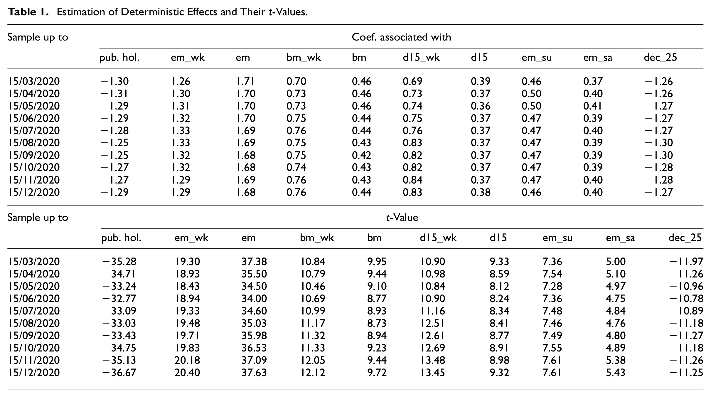
pub.hol.: public (bank) holidays,

em_wk: interaction of end of the month and weekend,

em: end of the month,

bm_wk: interaction of beginning of the month and weekend,

bm: beginning of the month,

d15_wk: interaction of day 15th of the month and weekend,

d15: day 15th of the month,

em_su: displacement of end of the month to previous Friday and Saturday when that day is Sunday,

em_sa: displacement of end of the month to previous Friday when that day is Saturday,

dec_25: December 25th, Christmas day.

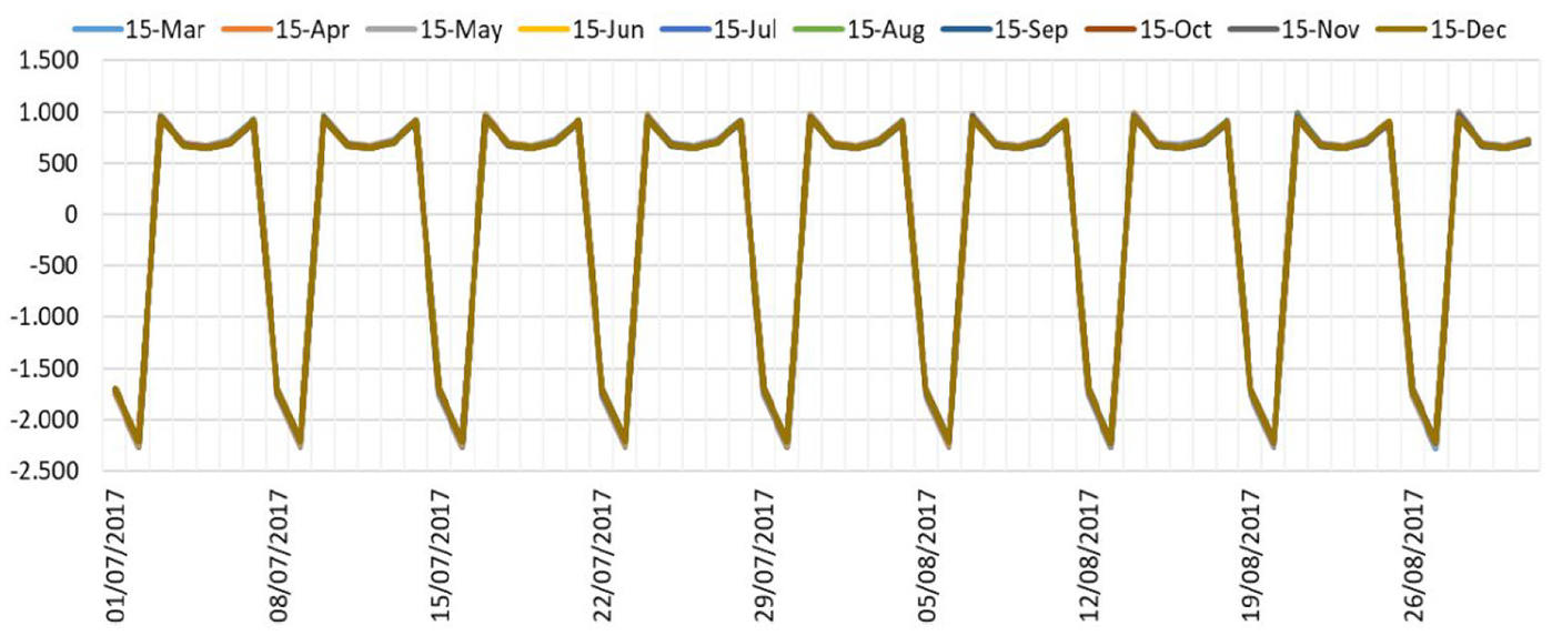
The displacement dummy variables em_su and em_sa require some explanation. When the last day of the month is a Saturday or a Sunday, part of the sales for the corresponding last day of the month is recorded the previous Friday (when Saturday) or the previous Friday and Saturday (when Sunday). Both variables are part of the interactions between the weekly and the monthly seasonal components. This effect is visible using the raw data when zooming the time frame, as can be seen in Figure 3.

Figure 3.

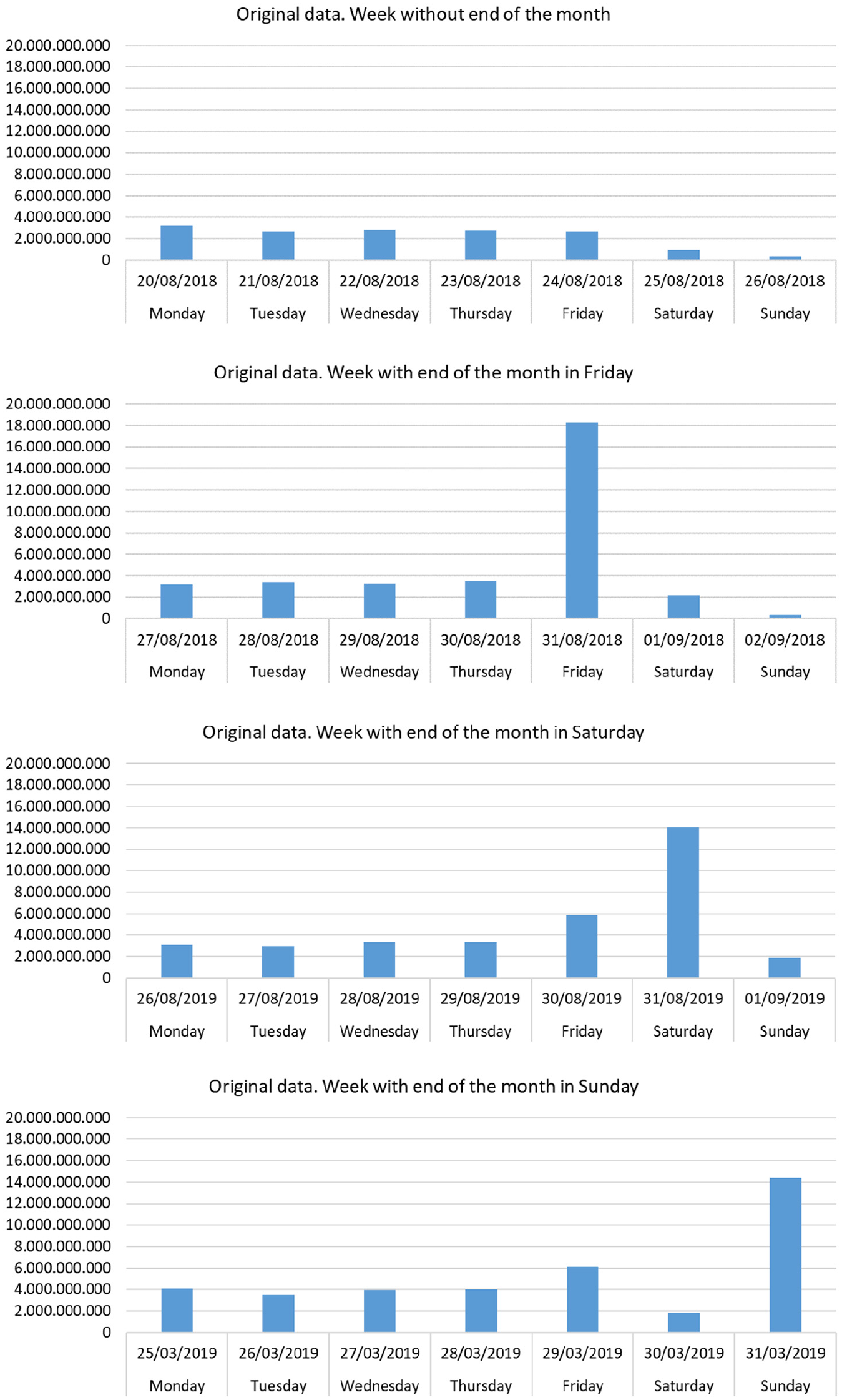
End of the month and weekends.

The first graph shows a “normal” week (i.e., without an end of the month day). In August 2019 it is visible a displacement of sales to Friday because the end of this month fell on a Saturday. This displacement did not happen in August 2018, when the end of the month was on a Friday. In the same way, when the end of the month is Sunday, a displacement to the previous Friday and Saturday is also visible.

As can be seen, the estimation of these effects is not particularly altered, nor is their significance. This supports the idea that the arrival of the CV19 strongly slowed down the turnover of the sectors especially exposed, the turnover of the sectors that remained in operation maintained their invoicing and recording patterns as in the previous period, especially at the beginning, middle, and end of the month. Note that the interaction effects are estimated with less precision than the corresponding basic effects, partly due to their comparative lower number of occurrences.

Once the series have been corrected from these deterministic effects, the representation of the non-observable components estimated with the samples up to the different periods can be seen in the following figures.

These graphs reveal that the estimation of the trend component is significantly affected from the first moment of the lockdown. In fact, it seems to show some induced annual seasonality, as well as an increase in its volatility. Obviously, this has its counterpart in the estimation of the annual seasonal component, which is also strongly modified. On the other hand, both weekly and monthly seasonality seem to resist well the presence of shock.

Table 2 presents the estimates of the TBATS parameters across vintages, completing the graphical results just commented.

Table 2.

TBATS Parameters Across 2020 Vintages.

Trend		Seasonality									Irregularity
Sample up to	α	Weekly			Monthly			Annual			ARMA(p,q)
		<k>	ϒ₁	ϒ₂	<k>	ϒ₁	ϒ₂	<k>	ϒ₁	ϒ₂	σ	p	q
15-Mar	0.014	3	0.001	0.002	6	0.000	0.001	11	−0.003	−0.001	0.129	0	0
15-Apr	0.050	3	0.002	0.002	6	−0.001	0.002	6	−0.002	−0.002	0.146	0	0
15-May	0.102	3	0.001	0.003	7	−0.001	0.002	4	−0.003	−0.005	0.151	0	0
15-Jun	0.051	3	0.002	−0.001	7	−0.001	0.002	8	−0.002	−0.002	0.142	0	0
15-Jul	0.068	3	0.001	0.003	7	−0.001	0.001	5	−0.002	−0.003	0.145	0	0
15-Aug	0.076	3	0.002	0.001	7	−0.001	0.001	5	−0.003	−0.003	0.145	0	0
15-Sep	0.057	3	0.001	0.001	7	−0.001	0.001	8	−0.003	−0.002	0.138	0	0
15-Oct	0.053	3	0.000	0.002	6	−0.001	0.001	8	−0.003	−0.001	0.138	0	0
15-Nov	0.054	3	0.001	0.001	6	−0.001	0.001	8	−0.002	−0.002	0.137	0	0
15-Dec	0.051	3	0.000	0.002	6	−0.001	0.001	8	−0.003	−0.001	0.140	0	0

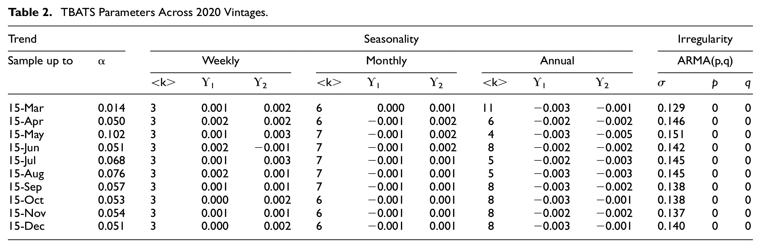
Some comments on this table:

The scale parameter of the trend, $α$ , is the most affected by the CV19 shock, increasing on average four times with respect to its pre-CV19 estimates. This explains the dramatic changes seen in Figure 4.

On the opposite side, the scale parameters of the weekly seasonal component reduce their (absolute) estimates, indicating a quasi-deterministic behavior. In addition, the number of harmonics remains constant. This explains the notable stability seen in Figure 5.

In an intermediate position, both the monthly seasonality and, especially, the annual seasonality show an increased sensitivity with respect to the innovation (higher scale parameters) as well as some instabilities regarding the number of harmonics. This explains the changes observed in Figures 6 and 7.

The sharp decrease in the number of harmonics of the annual seasonal component, from 11 (15-Mar vintage) to 6 (15-Apr vintage) and the progressive, albeit incomplete, recovery to 8 (from the 15-Sep vintage onwards), is in broad agreement with the qualitative profile of the CV19 shock.

Across vintages, TBATS always considered the shocks that define the irregular component as white noise (p = q = 0).

Finally, the overall size of the shocks has increased too, as reflected in the higher values of the σ parameter.

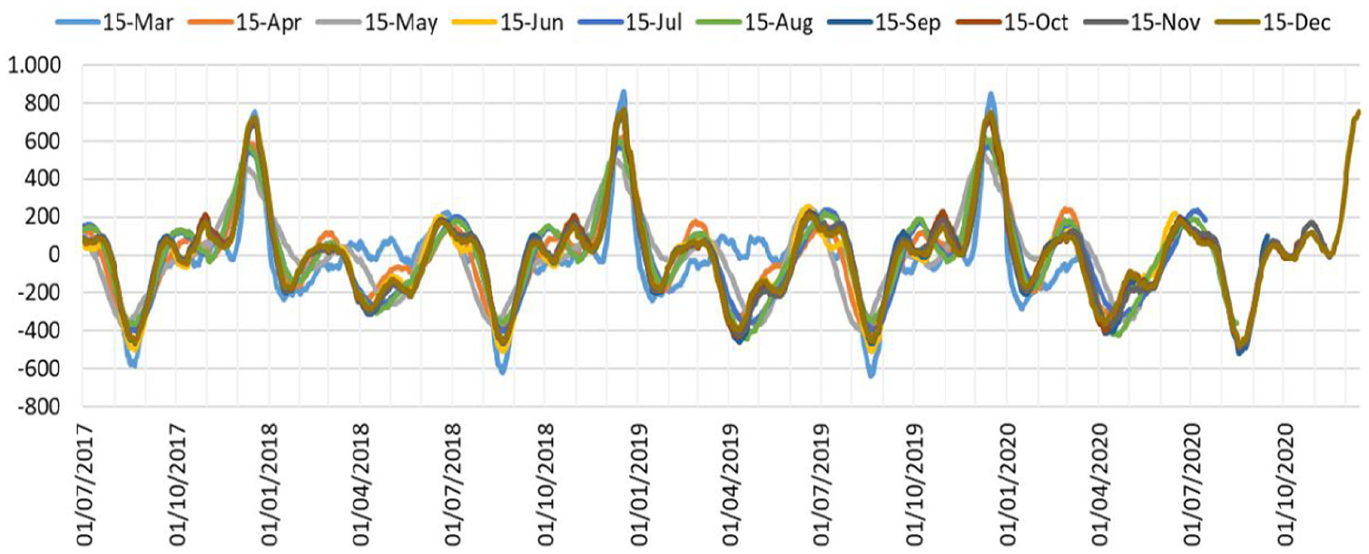
In any case, this alteration in the decomposition significantly affects the seasonal and calendar adjusted (SAC) series, which are the most popular and relevant for the monitoring of the short-term conjuncture. Although it is more difficult to visualize due to the strong irregular component of the sales data (see Figure 8 for the representation of the original and SAC series), Figure 9 shows the important changes in the seasonal and calendar adjusted series for the first two time periods considered.

Figure 4.

Trend estimates (million EURO).

Figure 5.

Weekly seasonality estimates (million EURO). Sample: 01/07/2017 to 31/08/2017.

Figure 6.

Monthly seasonality (stochastic) estimates (million EURO). Sample: 01/07/2017 to 31/08/2017.

Figure 7.

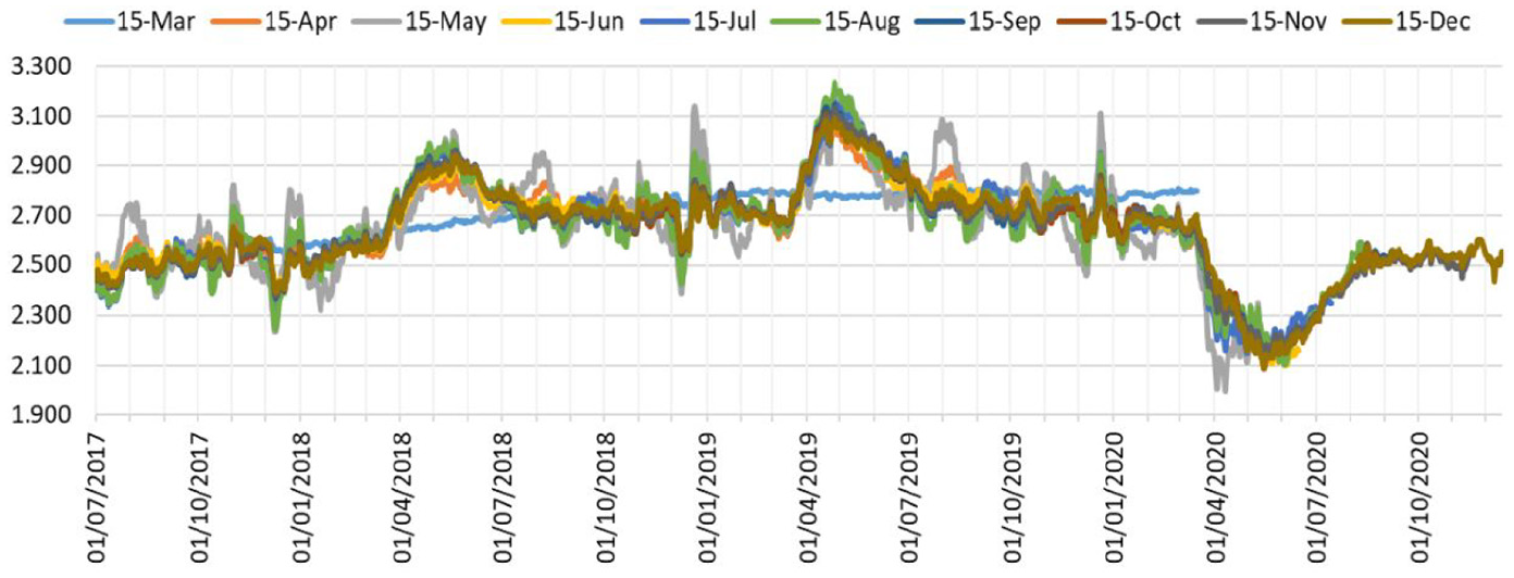
Annual seasonality estimates across vintages (million EURO).

Figure 8.

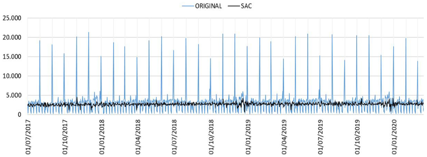
Original and seasonal and calendar adjusted series (million EURO).

Figure 9.

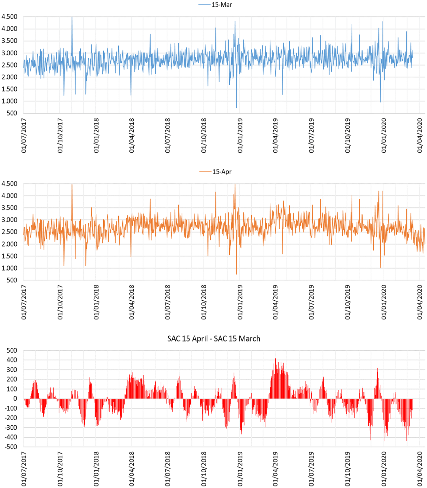
Seasonal and calendar adjusted series (million EURO) in 15/03/2020 and 15/04/2020.

Therefore, the previous graphs recommend setting the focus of the analysis on a component such as the trend, which is less sensitive with respect to irregular elements.

4.2. Real-Time Processing Using the Pre-CV19 Model

As we have seen, the impact of the CV19 shock was noticeable very early. A simple and affordable way to mitigate its impact on the model and the decomposition that induces on the observed data is to keep the model fixed, using the estimated parameters from the pre-CV19 sample to perform the correction from deterministic effects (linearization step) and the decomposition into trend, three seasonal factors and a remainder (TBATS step).

The next graph shows the trend estimates from the different vintages, using the parameters estimated from the pre-CV19 sample for the regression model (step 1) as well as for the TBATS model (step 2). From now on, we will set the focus on the trend component since it is the most sensitive with respect to the shocks (Cuevas et al. 2021) and to enhance the graphical analysis due to the strong irregular component of the sales data (Figure 10).

Figure 10.

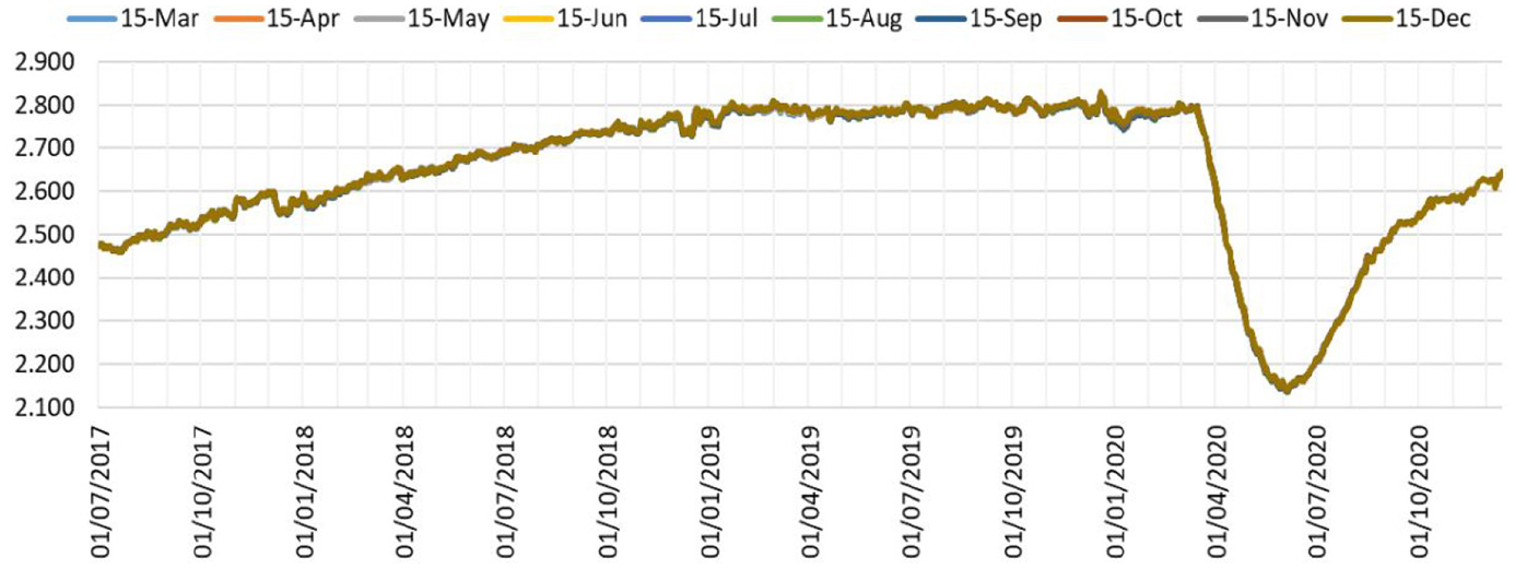
Trend estimates using the model from pre-CV19 sample (million EURO).

The estimates are remarkably stable, preserving the pre-CV19 estimates and thus providing a homogeneous measure of the strength of the CV19 shock. They are not completely stable due to the workings of the smoothing pass of the Kalman filter that is applied to the same time series but with differing lengths.

This procedure provides a simple and sensible way to avoid the disruptive effects of the CV19 shock on the model and the estimated components. However, is this solution permanent?

Once the lockdown ended, the Spanish economy entered uncharted waters. On the one hand, the strict lockdown finished but the new measures then introduced posed an environment clearly different from the pre-CV19 one, due to the restrictions imposed on mobility, limits on capacity and activity, general health measures, etc.

This “new normal” state of affairs was also inhomogeneous from a regional perspective (e.g., some small islands in the Canary and Balearic archipelagos reached less restrained conditions sooner than the large cities in the Peninsula) as well as from a sectoral perspective (e.g., the constraints were stricter for activities linked to social consumption than for the industry and construction activities). This lack of homogeneity poses new difficulties from a modeling perspective. On the one hand, we knew that “new normal” was far different from “normal” but, on the other hand, it was also clear that it was far less strict than the lockdown phase.

4.3. Setting a Flexible Intervention Variable

A more correct and sophisticated solution is to introduce a specific regression variable to represent the shock of CV19 in its deepest phase, which allows a correct decomposition of seasonal factors. Subsequently, this regression variable would be assigned to the trend component.

Obviously, the most correct specification of this variable can only be made when the duration of the shock is known a posteriori.

In this case, the form of the regression variable chosen was as the “tent” type, with the functional form expressed in Equation (12) and represented as an example in Figure 11.

I_{t} (τ; δ_{1}, δ_{2}) = {\begin{matrix} \frac{1}{1 - δ_{1} F} \\ 1 \\ \frac{1}{1 - δ_{2} B} \end{matrix}} \leftrightarrow {\begin{matrix} t < τ \\ t = τ \\ t > τ \end{matrix}}

(12)

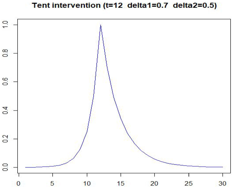
For its full determination, a search algorithm of the parameters is proposed. A succession of regressions of the series corrected from deterministic effects on the intervention variable is run, including a deterministic trend and the seasonal Fourier variables determined by the harmonics of the first stage. In these regressions $δ_{1}$ and $δ_{2}$ vary in the range 0.01 to 0.99 and $τ$ varies between March 1 and June 30. Finally, we keep the combination that minimizes the AIC, thus determining the optimum of these parameters. In our case, the minimum is reached at $τ$ = March 28 (see Figure 12), $δ_{1} = 0.88$ and $δ_{2} = 0.99$ .

Figure 11.

Type of “tent” intervention variable for CV19.

Figure 12.

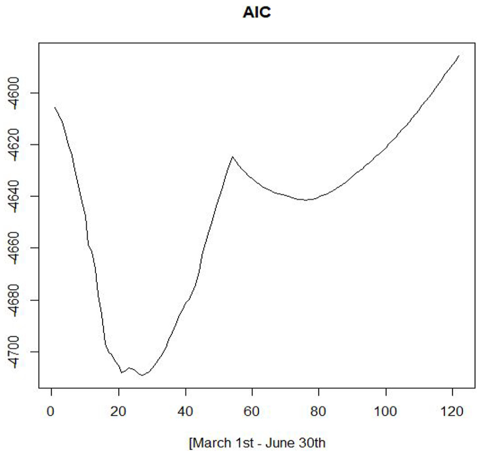
Minimum AIC.

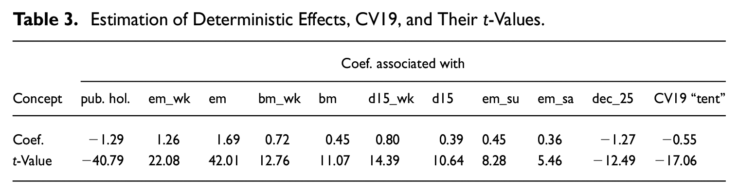
The estimation with the sample up to December 15, 2020, including the CV19 variable is summarized in Table 3.

Table 3.

Estimation of Deterministic Effects, CV19, and Their t-Values.

	Coef. associated with
Concept	pub. hol.	em_wk	em	bm_wk	bm	d15_wk	d15	em_su	em_sa	dec_25	CV19 “tent”
Coef.	−1.29	1.26	1.69	0.72	0.45	0.80	0.39	0.45	0.36	−1.27	−0.55
t-Value	−40.79	22.08	42.01	12.76	11.07	14.39	10.64	8.28	5.46	−12.49	−17.06

In addition, the search exercise has been carried out with a succession of regressions of the original series on the intervention variable, the deterministic effects, a deterministic trend, and the seasonal Fourier variables determined by the harmonics of the first stage. The results are quite similar, with the minimum reached at $τ$ = March 30, $δ_{1} = 0.88$ , and $δ_{2} = 0.99$ .

Obviously, the coefficient of the CV19 variable is highly significant. Compared to not introducing it, the changes are very clear in the following figures, showing a great improvement (Figure 13).

Figure 13.

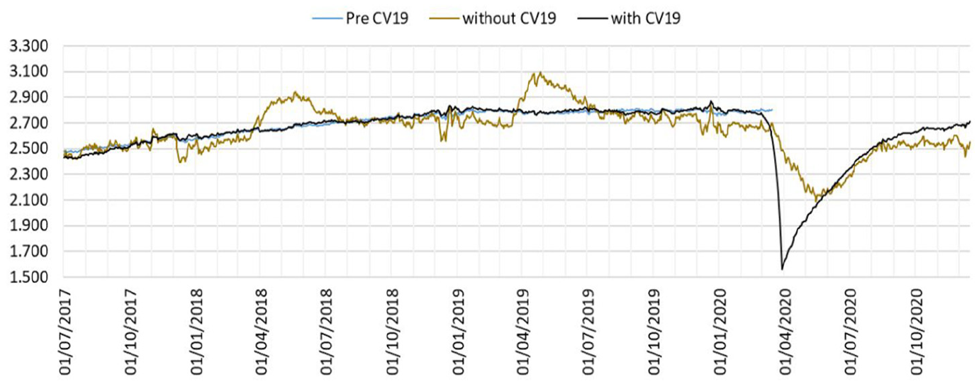
Trend estimates, pre-CV19 and full sample, with and without CV19 “tent” intervention variable.

As can be seen, the estimation of the trend recovers the stability that is assumed, while the annual seasonal component is more similar to that of the pre-CV19 period, without marking those falls in April-May that were transmitted to the trend component. However, this recovery is not complete as can be seen in the reduced amplitude of the mid-Summer and turn-of-the-year peaks, although the underlying time profile is kept.

Additionally, this difference is very evident when comparing the fixed-model estimates with the estimates derived from a free-model plus CV19 intervention. Figure 14 shows this difference.

Figure 14.

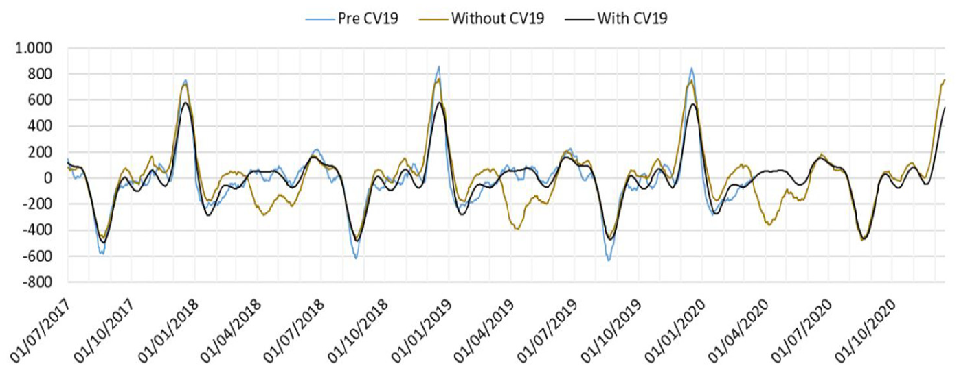
Annual seasonality estimates, pre-CV19 and full sample, with and without CV19 “tent” intervention variable.

The fixed-model estimates provide a very good directional image of the underlying economic conditions but with a certain delay and a remarkable underestimation. Both estimates are very close to the pre-CV19 estimates, suggesting that the underlying dynamics remain the same, once one-off shocks like the CV19 one are taken into account.

Of course, the free model plus CV19 intervention can only be implemented once we have a sufficient sample, that is, only with the benefit of hindsight. On a real-time basis, we have to rely on biased but stable estimates as those provided by the model estimated with the pre-CV19 sample (Figure 15).

Figure 15.

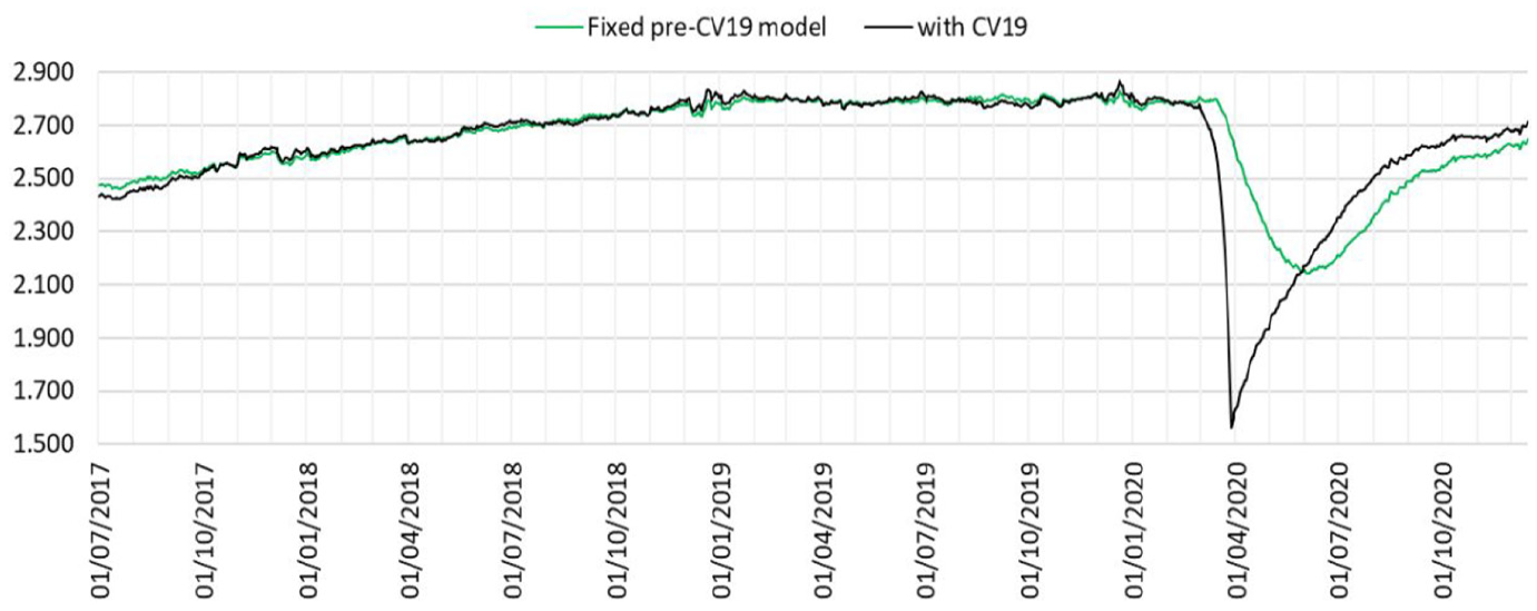
Trend estimates using the pre-CV19 model versus full sample model plus CV19 intervention.

4.4. Alternative Intervention: Piecewise Step Intervention

As we have seen, the nature of the CV19 shock allows us to define two intervention (dummy) variables since its onset. The first one (lockdown) is set to one during the most stringent phase (from March 15th to May 26th) and the second one (new normal) is set to one once the lockdown ended (from May 27th onwards). The beginning and the end of the lockdown phase were determined by the Spanish Government declaring an emergency state.

As can be seen in the next graph, the real-time coefficient estimates of the lockdown effect are sizeable and very stable since the very beginning, in close agreement with its exceptional, sharp, and strong impulse. On the contrary, the new-normal intervention is less stable, suggesting an upward movement consistent with the progressive recovery of the sales data. Note that this recovery is clearly incomplete due to the prevalence of its negative sign and its distance from zero at the end of 2020 (Figure 16).

Figure 16.

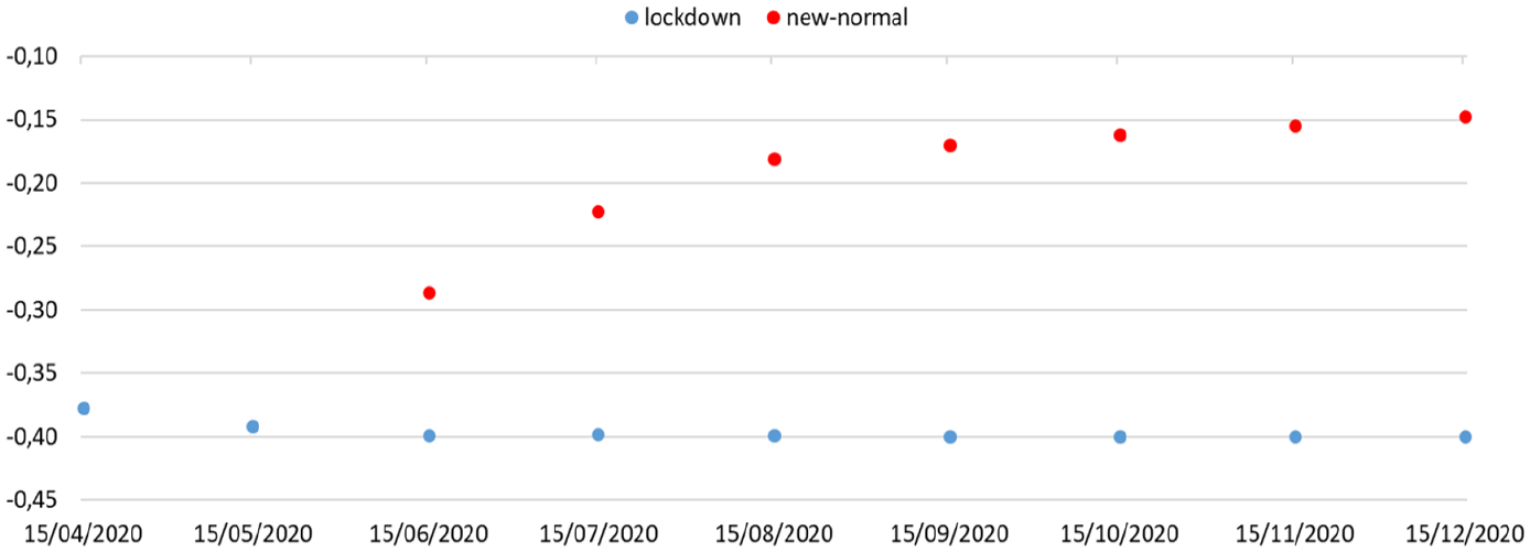
Real-time coefficient estimates of the lockdown and new-normal interventions.

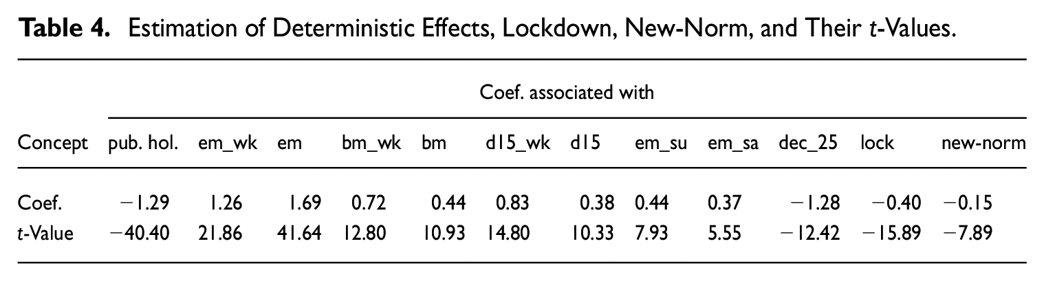
The estimates of the remaining deterministic effects are fairly robust with respect to the lockdown and new-normal interventions, as can be seen in the Table 4.

Table 4.

Estimation of Deterministic Effects, Lockdown, New-Norm, and Their t-Values.

	Coef. associated with
Concept	pub. hol.	em_wk	em	bm_wk	bm	d15_wk	d15	em_su	em_sa	dec_25	lock	new-norm
Coef.	−1.29	1.26	1.69	0.72	0.44	0.83	0.38	0.44	0.37	−1.28	−0.40	−0.15
t-Value	−40.40	21.86	41.64	12.80	10.93	14.80	10.33	7.93	5.55	−12.42	−15.89	−7.89

The combined effect of both interventions is a piecewise factor very strong during two months (lockdown) and milder during the new-normal phase but still negative. However, this combined effect provides and incomplete picture of the full sample estimation using the CV19 intervention, as can be seen in Figure 17.

Figure 17.

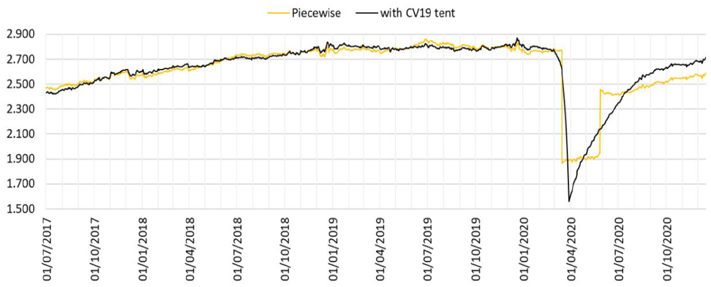
Trend estimates: piecewise versus CV19 “tent” intervention variables.

The estimates provide a more accurate gauge of the impact of the CV19 shock during its strongest phase (lockdown) but overstates its persistence, underestimating the strength of the recovery. In any case, it provides a benchmark to qualify the estimates provided by the model fixed at its pre-CV19 estimates.

4.5. Alternative Intervention: Lockdown Plus “Tent” Intervention

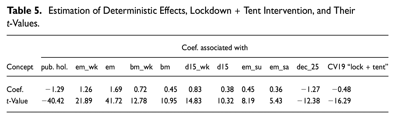
An alternative that could be feasible is to propose an intervention variable that is the combination of a lockdown period plus a progressive recovery “tent” type variable. The results of its estimation and the derived trend are shown in Table 5 and Figure 18.

Table 5.

Estimation of Deterministic Effects, Lockdown + Tent Intervention, and Their t-Values.

	Coef. associated with
Concept	pub. hol.	em_wk	em	bm_wk	bm	d15_wk	d15	em_su	em_sa	dec_25	CV19 “lock + tent”
Coef.	−1.29	1.26	1.69	0.72	0.45	0.83	0.38	0.45	0.36	−1.27	−0.48
t-Value	−40.42	21.89	41.72	12.78	10.95	14.83	10.32	8.19	5.43	−12.38	−16.29

Figure 18.

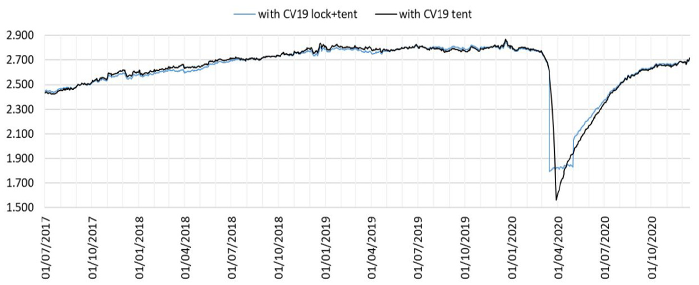
Trend estimates: CV19 “lockdown + tent” versus CV19 “tent” intervention variables.

The results of the estimate remain stable and the combined variable is fully significant. However, comparing it with the “tent” intervention variable, is slightly less significant, while it could seem that it results in a less continuous profile. For this reason, we finally prefer to stay with the “tent” variable type as the best option. However, as can be seen in the Appendix A, the residual diagnostics of the different specifications favor slightly the “Lockdown + tent” CV19 intervention.

5. Conclusions

From a practitioner’s view, the CV19 shock greatly affects the model and the corresponding decomposition of the observed daily sales data. We present here some conclusions derived from our experience when dealing with the CV19 shock during the last two years.

The pre-processing (or linearization) step is very important. The correction from deterministic effects linked to the interaction between seasonal components (weekly and monthly) as well as to the special nature of the monthly seasonality, plays a critical role in ensuring a homogeneous and properly structured input for the decomposition performed in the second step. Fortunately, the estimates of these deterministic effects, including bank holidays, are very stable, significant and robust with respect to outliers, including those related to the CV19 shock.

The CV19 shock has a major impact on the decomposition of the corrected daily time series, destabilizing the trend and the annual seasonality and generating a wrong attribution of the CV19 shock to the annual seasonality. Weekly and monthly seasonality remains practically unaffected by the CV19 shocks.

Shocks like CV19 pose an extraordinary challenge for short-term monitoring on a real-time basis. Their destabilizing effects are quickly detected and a simple, preemptive measure is to keep the estimated pre-shock model fixed while processing the incoming, shocked observations. While this procedure is somewhat biased, it preserves very well the overall direction of the changes and gives a clear picture of the relative cross-sectional effects of the CV19 shock (e.g., the comparison between industrial and services activities). Obviously, this solution is temporary because we cannot keep fixed the model forever.

The above procedure can be improved by means of an intervention analysis. In this way, the initial lockdown was modeled by means of a level shift. This approach produces an updated estimate of the effects but it is more prone to revisions.

The CV19 shock has been largely unusual due to its huge size and its sharp effects but it can be clearly linked to exogenous events with known and public dates of occurrence, like the starting and ending dates of lockdowns and other constraints on mobility and capacity. The exogenous and quasi-deterministic nature of the CV19 shock makes it amenable for a classical intervention analysis (Box and Tiao 1975). In this way, two years after its initial impact, we can represent most of it by means of a single, two-sided transitory change intervention (a “tent” type variable). We have presented here some additional tests aimed at qualifying this approach.

The accumulation of empirical experience, theoretical developments, and specific computational tools will surely improve modeling daily economic time series. For future work, we plan to compare TBATS with non-parametric filtering methods, as in Ollech (2021) and to explore procedures for the automatic detection and removal of outliers designed for the special features of daily economic time series.

Footnotes

Appendix A

Acknowledgements

We thank J. Abelaira, R. Frutos, D. García, and R. Ledo for their input at different stages of this project. We also thank the anonymous referees for their comments and suggestions that have contributed to improve notably the text. The opinions are those of the authors and do not necessarily reflect the views of the Spanish Tax Agency.

Funding

The author(s) received no financial support for the research, authorship, and/or publication of this article.

ORCID iD

Enrique M. Quilis

References

Bell

W. R.

Hillmer

S. C.

1983. “Modeling Time Series with Calendar Variation.” Journal of the American Statistical Association 78 (383): 526–34. DOI: https://doi.org/10.1080/01621459.1983.10478005.

Box

G. E. P.

Tiao

G. C.

1975. “Intervention Analysis with Applications to Economic and Environmental Problems.” Journal of the American Statistical Association 70 (349): 70–9. DOI: https://doi.org/10.1080/01621459.1975.10480264.

Cuevas

Á.

Ledo

Quilis

E. M.

2019. “Incorporando información fiscal de frecuencia diaria en la previsión macroeconómica a corto plazo.”Instituto de Estudios Fiscales, Papeles de Trabajo, #11/2019. https://www.ief.es/docs/destacados/publicaciones/papeles_trabajo/2019_11.pdf (accessed September 3, 2024).

Cuevas

Á.

Ledo

Quilis

E. M.

2021. “Seasonal Adjustment of the Spanish Sales Daily Data.” SERIEs 12: 687–708. DOI: https://doi.org/10.1007/s13209-021-00251-7.

De Livera

Hyndman

R. J.

Snyder

R. D.

2011. “Forecasting Time Series with Complex Seasonal Patterns Using Exponential Smoothing.” Journal of the American Statistical Association 106 (496): 1513–27. DOI: https://doi.org/10.1198/jasa.2011.tm09771.

Espasa

Revuelta

J. M.

Cancelo

J. R.

1996. “Automatic Modelling of Daily Series of Economic Activity.” In Proceedings in Computational Statistics, edited by Prat

, 51–63. Berlin: Physica-Verlag. DOI: https://doi.org/10.1007/978-3-642-46992-3_5.

Eurostat. 2020. “Guidance on Time Series Treatment in the Context of the Covid-19 Crisis.”Methodological Note. https://ec.europa.eu/eurostat/documents/10186/10693286/Time_series_treatment_guidance.pdf (accessed September 3, 2024).

Harvey

A. C.

1989. Forecasting, Structural Time Series Models and the Kalman Filter. Cambridge: Cambridge University Press. DOI: https://doi.org/10.1017/CBO9781107049994.

Hillmer

S. C.

Bell

W. R.

Tiao

G. C.

1983. “Modeling Considerations in the Seasonal Adjustment of Economic Time Series.” In Applied Time Series Analysis of Economic Data, edited by Zellner

, 74–100. Washington, DC: US Bureau of the Census. https://www.census.gov/content/dam/Census/library/working-papers/1983/adrm/hillmerbelltiao1983.pdf (accessed September 3, 2024).

10.

Hyndman

R. J.

2017. “Monthly Seasonality.” Blog Entry in “Hyndsight Blog.”https://robjhyndman.com/hyndsight/monthly-seasonality/index.html (accessed September 3, 2024).

11.

Hyndman

R. J.

Khandakar

2008. “Automatic Time Series Forecasting: The Forecast Package for R.” Journal of Statistical Software 27 (3): 1–22. DOI: https://doi.org/10.18637/jss.v027.i03.

12.

Kim

C. J.

Nelson

C. R.

1999. State-Space Models with Regime Switching. Cambridge, MA: MIT Press. DOI: https://doi.org/10.7551/mitpress/6444.001.0001.

13.

Ladiray

Palate

Mazzi

G. L.

Proietti

2018. “Seasonal Adjustment of Daily and Weekly Data.” In Handbook on Seasonal Adjustment, edited by Ladiray

Mazzi

G. L.

Luxembourg: Eurostat. https://ec.europa.eu/eurostat/documents/3859598/8939616/KS-GQ-18-001-EN-N.pdf/7c4d120a-4b8a-441b-aefd-6afe81a7cf59?t=1533194231000 (accessed September 3, 2024).

14.

Leiva-León

Pérez-Quirós

Rots

2020. “Real-Time Weakness of the Global Economy.” Working Paper n. 2381, European Central Bank. https://www.ecb.europa.eu/pub/pdf/scpwps/ecb.wp2381∼444d6f578f.en.pdf (accessed September 3, 2024).

15.

Lenza

Primiceri

2020. “How to Estimate a VAR AfterMarch 2020.” Working Papers n. 27771, NBER. DOI: https://doi.org/10.3386/w27771.

16.

Liu

L. M.

2005. Time Series Analysis and Forecasting. River Forest, IL: Scientific Computing Associates.

17.

Maroz

Stock

J. H.

Watson

M. W.

2021. “Comovement of Economic Activity During the Covid Recession.”Forecasting in a Changing Environment, International Institute of Forecasters, International Symposium, Madrid, December 9–10. https://www.princeton.edu/~mwatson/papers/Covid_Factor_20211215.pdf (accessed September 3, 2024).

18.

2021. “Modeling Macroeconomic Variations After Covid-19.” Working Papers n. 29060, NBER. DOI: https://doi.org/10.3386/w29060.

19.

O’Hara-Wild

Hyndman

Wang

2024. “Package fable: Forecasting Models for Tidy Time Series.”https://fable.tidyverts.org/ (accessed September 3, 2024).

20.

Ollech

2021. “Seasonal Adjustment of Daily Time Series.”Journal of Time Series Econometrics 13 (2): 235–64. DOI: https://doi.org/10.1515/jtse-2020-0028.

21.

Primiceri

G. E.

Tambalotti

2020. “Macroeconomic Forecasting in the Time of COVID-19.” Working Paper, Northwestern University. https://faculty.wcas.northwestern.edu/gep575/PredictionCovid1-5.pdf (accessed September 3, 2024).

22.

Schorfheide

Song

2020. “Real-Time Forecasting with a (Standard) Mixed-Frequency VAR During a Pandemic.” Working Paper n. 20-26, Federal Reserve Bank of Philadelphia. DOI: https://doi.org/10.21799/frbp.wp.2020.26.

23.

Tax Agency. 2017. “Daily Domestic Sales.”Spanish Tax Agency. https://sede.agenciatributaria.gob.es/Sede/en_gb/estadisticas/ventas-empleos-salarios-declaraciones-tributarias/ventas-diarias.html (accessed September 3, 2024).

24.

Ten

G. K.

Merfeld

Hirfrfot

K. T.

Newhouse

Pape

2022. “How Well Can Real-Time Indicators Track the Economic Impacts of a Crisis Like COVID-19?” Working Paper n. 10080, World Bank. DOI: https://doi.org/10.1596/1813-9450-10080.

The COVID-19 Shock Through the Lens of the Spanish Sales Daily Data: Modeling and Seasonal Adjustment Challenges

Abstract

Keywords

1. Introduction

2. Data

3. Modeling Daily Data

3.1. Pre-Processing (Linearization)

3.2. Structural (TBATS) Decomposition

4. Measuring the Impact of the CV19 Shock

4.1. Estimation Effects of the CV19 Shock

4.2. Real-Time Processing Using the Pre-CV19 Model

4.3. Setting a Flexible Intervention Variable

4.4. Alternative Intervention: Piecewise Step Intervention

4.5. Alternative Intervention: Lockdown Plus “Tent” Intervention

5. Conclusions

Footnotes

Appendix A

Acknowledgements

Funding

ORCID iD

References