
Abstract
We introduce a novel seasonal adjustment methodology developed by Quantcube Technology, termed Seasonal, Trend, and Holiday Decomposition with Loess (STAHL). This method builds upon the STL procedure outlined by Cleveland et al. and is tailored for application to time series across varying frequencies. Initially, we detail the innovations introduced by STAHL, which include the spectral identification of multiple seasonal frequencies and the systematized preprocessing different seasonal series. This preprocessing encompasses resampling, real-time handling of missing values, and other necessary adjustments. Additionally, we illustrate how the holiday decomposition component effectively manages the variability of moving holiday events. In addition to this, we introduce the Barnacle procedure, to deal with before and after effects of holiday. Subsequently, we provide empirical demonstrations using high frequency data. Specifically, we utilize US Weekly initial claims data to exemplify real-time adjustments during the unprecedented COVID-19 period, with comparisons to the series adjusted by the US Department of Labor. Furthermore, daily Google search data for the term “Easter bunny” illustrate our method’s capability in handling moving holiday effects. We also perform a simulation study to compare the performance of STAHL with existing high frequency seasonal adjustment methodologies.
Keywords
1. Introduction
Macroeconomic nowcasting has increasingly involved the use of various types of massive data over the past decade, which include non-traditional sources of high frequency information that can provide unique insights. They can be clustered into four major categories: text data, geospatial data, geolocation data, and structured data. Text data can be recovered via multiple channels, such as the internet, social media data, professional blogs, news articles, job ads, web searches, or hotel and restaurant reviews. Non traditional high frequency time series such as textual or web search data have for instance been the focus of extensive research in the nowcasting literature like in D’Amuri and Marcucci (2017) and Aprigliano et al. (2023).
The availability of high-resolution satellite imagery and the development of deep learning models have led to numerous applications allowing the recovery of various geospatial data from earth observation satellite images, atmospheric data, or radar data. Geolocation data can take the form of shipping traffic, flights, mobility, or vehicle transit numbers. Structured data can encompass prices of goods and services, real estate prices, internet queries, and web traffic.
Quantcube Technology aims to provide a competitive edge by uncovering hidden patterns, detecting emerging trends, and enhancing predictive models by leveraging all those non-traditional data sources. Most of these data are produced at a daily frequency, seven days a week, without exception. These time series exhibit a rather short history, oscillating between five and just over ten years. As such, their statistical analysis must address many specific issues. A primary problem to tackle is the complexity of the multiplicity and potential interactions of seasonal patterns (notably annual, monthly, weekly, and daily cycles) and calendar effects (such as holidays, and time-varying non-Gregorian calendars like the Chinese or Hijri calendars).
Furthermore, those non-traditional data may suffer from high sensitivity to outliers at high frequencies, such as mobility bans during the COVID periods, and may be prone to periodic or structural missing values, like clouds disturbing the quality of satellite images at regular intervals. In addition, most financial and macro practitioners expect those data sources used for nowcasting to be timely delivered and unrevised, which presents a specific practical challenge from a seasonality extraction perspective. This article aims to precisely tackle all these reported issues by introducing a new seasonal adjustment framework: Seasonal, Trend, and Holiday Decomposition based on LOESS (STAHL).
We begin with a literature review in Section 2 were we examine the current literature on seasonal adjustment and give an overview of the methods that are currently available. We discuss their pros and cons from a practitioner’s point of view, aiming at an automated and methodical daily production of seasonally adjusted non-traditional data. We particularly focus on the STL (Seasonal-Trend Decomposition based on LOESS) approach and discuss why we consider an extended version of this procedure as the best compromise for point-in-time seasonal adjustment of high frequency data. In Section 3 we present the STAHL framework. We explain how we modify the existing STL methodology to fit our specific requirement (e.g., point-in-time estimation). We also introduce the Holiday loop and the Barnacle procedure that let us deal with holidays, and their lead and lag effects. Next, in Section 4 we compare STAHL to TRAMO-SEATS, which is what we consider the current state of the art. Using a simulation study, we analyze how well the methods perform seasonal adjustment as well as holiday day adjustments. Several statistical tests are used to evaluate the performance of the two methodologies. Finally, Section 5 is devoted to empirical illustrations, where different types of high frequency data are studied with STAHL: weekly US initial unemployment claims and daily Google search volume. Both series provide interesting illustrations of the STAHL procedures, whether it is to produce point-in-time rolling seasonally adjusted series, manage outliers and extreme periods such as the COVID-19 episode, or address the impact of moving holidays such as Easter.
2. Seasonal Adjustment Methods for High Frequency Data:A Review
The digital transformation process of our modern economies and the outbreak of the COVID-19 pandemic have enhanced an interest for the statistical treatment of alternative and high frequency data. Infra-monthly economic data are in strong demand to provide more timely early warning economic nowcasting indicators which require to tackle specific statistical treatment. Webel (2022) has provided the most recent, to our knowledge, general and very exhaustive review of such methods.
Let’s note
While different parts of the literature focused on minute-by-minute, hourly, four-hourly data, we will focus on daily and weekly data in this exercise, as Quantcube Technology produces a large variety of those kind of HF series in an automated way seven days a week. At such frequencies, as described in Webel and Smyk (2024) there are already multiple difficulties arising due to interactions of calendar and seasonal effects which are almost absent at low frequencies. For example, the authors suggests that fixed-holiday and end-of-period effects may depend on the particular days of the week which the corresponding events fall onto. Christmas effects may be noticeably different for 24 to 26 December falling onto Tuesday through Thursday Friday through Sunday. The same applies to the short-lived end-of-Q3 elevation in level if the final day of that quarter had not been a Monday.
Adjusting for holidays becomes increasingly complex in countries where certain holidays, such as Islamic religious holidays, are determined by a calendar system distinct from the Gregorian calendar commonly used in everyday activities. Campante and Yanagizawa-Drott (2015) provide evidence that the Hijri (i.e., muslim) calendar, which is approximately 10 days shorter, impacts economic time series such as growth, mobility, and private consumption.
As illustrated in Webel (2022) or in Proietti and Pedregal (2023), the seasonal profile of HF time series is highly complex due to the coexistence of multiple and super-imposed seasonal patterns with integer and non-integer periodicities. (Seasonal periodicities of intra-weekly and shorter patterns will be integers but those of the monthly, quarterly, and yearly patterns will be non-integers when considered at daily frequency.)
The issue of data accessibility presents another quandary. Currently, higher frequency (HF) observations typically provide only a few years of history, which is often inadequate for reliably predicting all aspects of HF dynamics, including possible interaction effects. Conducting seasonal and calendar extraction on high frequency data through an automated and methodical approach, leveraging computational power to handle large volumes of information efficiently, is a challenge that must be addressed with as parsimonious a model as possible. Non-traditional HF data can also suffer from a significant amount of missing values, due either to measurement issues or holiday unavailability. This adds another constraint to the seasonal adjustment method, which must be able to deal with both regular and irregular patterns of missing values.
2.1. Extending Conventional Methods from the X11 Family to TRAMO-SEATS
Numerous statistical organizations worldwide use one of several recognized methods for seasonally-adjusting low frequency (LF) time series. These methods include the X11 approach, the AutoRegressive Integrated Moving Average (ARIMA) model-based strategy, and the Structural Time Series (STS) models.
Ladiray et al. (2018) detailed the challenges to adapt the “X11 family” seasonal adjustment procedure first introduced in Ladiray and Quenneville (2012) to HF data, but also the STL (Seasonal-Trend Decomposition using LOESS) introduced by R. B. Cleveland et al. (1990). They show that the main seasonal adjustment methods used for monthly and quarterly series, such as TRAMO-SEATS and X12-ARIMA, as well as STL, can be adapted to high frequency data which present multiple and non integer periodicities. For instance, TRAMO-SEATS can be modified using fractional ARIMA models and more efficient numerical algorithms. The non-parametric and iterative processes of X11 and STL can also be adapted after imputation of the missing values induced by the different lengths of months and year. But the authors argue that the tuning of the multiple parameters of the methods might be cumbersome.
More recently, Webel and Smyk (2024) discusses extensions to the TRAMO-SEATS seasonal adjustment methodology to handle infra-monthly (higher than monthly frequency) time series data in JDemetra+ 3.0. This software version can handle multiple seasonal patterns (e.g., daily, weekly, annual), dealing with fractional periodicities. It provides options for both sequential and simultaneous component estimation and implement robust outlier detection methods.
The main adaptations to TRAMO-SEATS for high-frequency data include
an Extended Airline Model (EAM) which allows for multiple seasonal patterns and fractional periodicities and uses first-order Taylor approximation to handle fractional powers of backshift operator,
a modified TRAMO-like pretreatment which handles calendar effects and outliers for high-frequency data and uses the EAM for modeling residuals,
an extended ARIMA Model-Based (AMB) approach, based on canonical decomposition of the EAM and which uses Kalman filter and smoother for signal extraction, and
an Extended X-11 approach which adapts classic 3 × 3 seasonal filters for fractional periodicities and incorporates new kernel-based trend-cycle filters.
Using three real high frequency datasets, Webel and Smyk (2024) show that EAM and the Structural Time Series (STS) approaches produced similar results for simpler series (daily births), that extended X-11 and STL gave comparable results for complex multi-seasonal patterns (hourly electricity), and that robust STL performed well in handling extreme COVID-19 effects without explicit modeling (weekly claims). As such this adaptation of TRAMO-SEATS is a great benchmark for an extended non-parametric approach based on STL to deal with moving holiday and outlier issues.
2.2. Structural Time Series Models and Its Variants
Proietti and Pedregal (2023) advocate for using Structural Time Series (STS) models on HF times series following the seminal modeling of Harvey and Koopman (1993) and Harvey et al. (1997). Unobserved Component Models (UCM) can, by design, handle any kind of high frequency data, but the models tend to be very “series specific” according to the authors. In particular, the selection of harmonics can be rather arbitrary and not that easy to conduct at scale. As a consequence, UCM models lack the desired flexibility we are looking for to implement an automated seasonal adjustment procedure that could be applied to a wide range of different type of data and frequencies. When testing UCM approaches, we notably experienced the same difficulties as indicated by Ollech (2021). We also faced severe identification and convergence issues in the maximum likelihood estimation of parameters. The optimization method may indeed exhibit convergence issues with high frequency data, leading to different local minima depending on the initialization, as pointed in Ladiray et al. (2018). This leads to issues with the identification of the signal-to-noise ratios of the idiosyncratic component, and the separation between the trend component and lower frequency seasonal components when considering STS and UCM models as a systematic solution for high frequency seasonal and calendar adjustment.
In the community of nowcasting and machine learning, Prophet, a Bayesian approach developed by Facebook’s Core Data Science team (Taylor and Letham 2018) is an often popular algorithm to conduct seasonal adjustment extraction. It has been particularly designed to provide a flexible and reliable forecasting tool that can be configured, interpreted, and evaluated by subject-matter experts and analysts without great expertise in time series modeling. The general idea is to specify relatively sparse Unobserved Component models and impose priors on the unknown parameters. There are many pros in favor of Prophet: it has been designed to detect yearly, weekly, and daily seasonality in data and to be robust to overfitting using regularization in the modeling process. It offers an intuitive way to include holidays, provided theirs effects are known and well identified. However, Prophet was more designed as a forecasting package rather than offering a general statistical decomposition framework. As such it often works as a black-box making it harder to understand the model intricacies. Furthermore, the Prophet framework does not currently allow the seasonal pattern to evolve with time, making it too restrictive for our macroeconomic daily series. Besides, trend extraction modeling is based on a non linear saturating growth and trend change detection approach which may also seem to be too restrictive, and not adapted to a point-in-time procedure.
2.3. Toward an Extended STL
According to Ollech (2021), the semi-parametric STL approach introduced in R. B. Cleveland et al. (1990) offers an alternative technique to extract HF series seasonality. Rooted in a locally weighted regression smoother (LOESS), it stands out from X11 due to its heightened flexibility concerning the frequency of the time series: STL can handle any type of frequency, not just monthly or quarterly.
A key strength of the STL algorithm, relative to STS, is its speedy computation, which enables the adjustment of varying seasonal frequencies within a unified iterative process, as well as being robust to outliers, making it suitable for data with anomalies. The primary purpose of STL is the decomposition of a time series into its trend, seasonal, and idiosyncratic components, making it straightforward to provide an interpretable decomposition. While it helps if the seasonal period is known, STL can be used without this knowledge, which can be a key strength when designing a systematic statistical decomposition framework. Given the simplicity of STL, it is somewhat easier to diagnose issues when they arise and to scale the approach. We will propose STAHL, an extended framework, to automatically assess holiday impacts in an integrated manner.
Ollech (2021) contributes to the existing literature by devising a seasonal adjustment routine for daily data, but also hints at STL’s limitations to single seasonal frequencies as it cannot deal with calendar effects such as the influences of moving holidays. Ollech (2021) also hints at convergence issues of the RegARIMA model for holiday adjustment of daily time series. Ollech (2021) also points at needed developments of STL to enhance its computational speed and reliability of the outlier detection and estimation. Webel (2022) takes also stock of needed automatic procedures to produce HF seasonal adjustments. The extended STL and X11 currently lack automatic selection rules for the seasonal filter given HF data. We found many studies about point-in-time versus in-sample seasonal estimates, and implied biases related to trend extraction, but to our knowledge there is no procedure fully dedicated to point-in-time seasonal adjustment, addressing notably asymmetric filtering problems. Our goal is notably to tackle those issues.
3. The STAHL Framework
Based on the well-known additive model STAHL decomposes a time series (

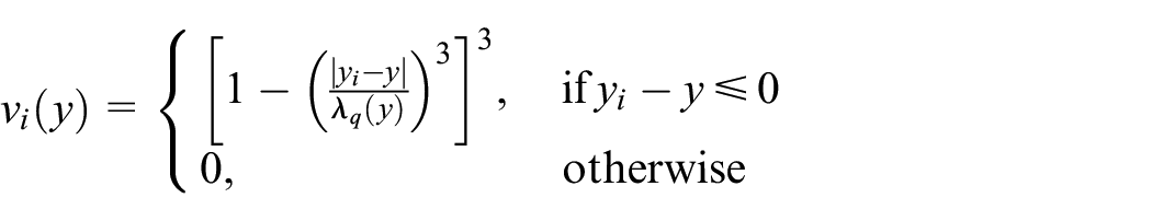
Each value is regressed in LOESS regressions on a local neighborhood of a linear fitted polynomials. For any point-in-time, the weight of the observation
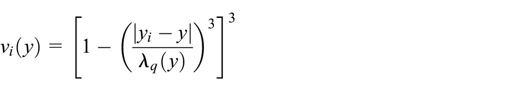
with
As illustrated in Figure 1, STAHL consists of a modified STL inner loop following the
Trend and Holiday adjustment.
Preliminary subseries smoothing by LOESS of bandwidth
Low-pass filter composed of moving average (Subsection 3.3) and LOESS asymmetric filters of bandwidth
First Seasonal Component :
First Seasonally adjusted Series :
First Trend Series
First idiosyncratic component:
At this stage, the idiosyncratic component may contain outliers and non-seasonal but regular holiday pattern effects. One of the key innovation with the STAHL framework is to add a second inner loop that will disentangle outliers from holiday estimations, and leads to a systemic construction of seasonally and holiday adjusted series.
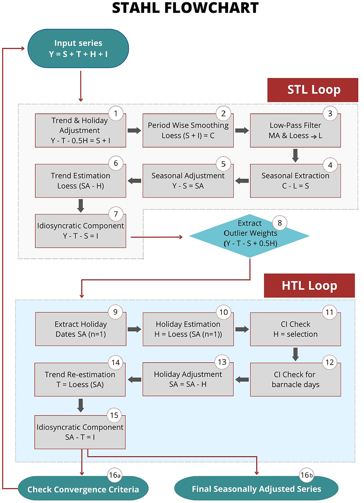
STAHL framework decomposition.
As introduced in the STAHL Flowchart in Figure 1, the HTL (Holiday Trend Decomposition Loop) works as follows:
08. Extraction of potential Holiday dates from
09. Holiday estimation,
10. Holiday selection with adjusted Confidence Interval (Appendix A.4.1)
11. Barnacle day selection with Barnacle procedure (Section 3.4.1)
12. Holiday Adjustment
13. Trend Reestimation
14. Reconstruction of the idiosyncratic:
Similarly to the STL framework, an outer loop is performed in order to prevent outlier contamination in the seasonal adjustment. The loop consists in extracting robustness weights
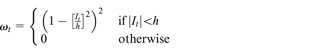
where
The robustness weights are then used as multipliers for the LOESS regression weights in the STL and HTL inner loops, significantly reducing the weights of outlier observations. This provides an automatic way to deal with additive outliers, temporary changes and temporary level shifts. However, there is currently no ad-hoc methodology to process ramps and level shifts in the STAHL framework. We could consider adding an intervention procedure similar to the one described in Chang et al. (1988) to solve this issue.
With this framework, the parameters of the procedure are the following:
3.1. STAHL Preprocessing Systematic Approach
3.1.1. Identification of Seasonality
Before setting any other parameter for the STAHL procedure, the first parameter to identify is
The methodology consists in creating
In practice, spectral density analysis may encounter challenges related to spectral leakage when attempting to accurately identify peaks. To address this issue and corroborate the presence of seasonality, we employ additional statistical tests in conjunction with the spectral density analysis. Specifically, we implement the QS-test Maravall (2012) and if needed, the Friedman test to provide robust confirmation of seasonal patterns. Furthermore, to ascertain whether the observed seasonality exhibits an additive or multiplicative nature, we conduct a visual inspection following the methodology described in W. S. Cleveland and Terpenning (1982). This approach involves examining the correlation between the amplitude of the seasonal component and the underlying trend.
3.1.2. Resampling of Data
By nature, the STAHL procedure can only be used for integer periodicities. While this is not a problem for monthly and quarterly data, in practice, the periodicities for weekly and daily data are mostly non-integers. To apply the procedure to high frequency data, we need to resample our data.
For daily data, we use the methodology described in Ollech (2021). To adjust for seasonality, the length of each month is extended to thirty-one days, either by time-warping the months over 31 points or by adding extra points at the end of each month using cubic spline interpolation, depending on the nature of the data. For annual seasonality, February 29th is removed to ensure a consistent 365 points per year before adjusting. Once the STAHL procedure has been applied to the resampled data, the resampling procedure is reversed: the added dates are removed, and the removed dates are added back using interpolation.
In the case of weekly data, the issue is slightly different because of the phasing effect of weeks in the year: the year does not always start on a specific day of the week. As the underlying annual seasonality is observed with a progressive shift, with fifty-two or fifty-three weeks per year. (Furthermore for economic data, the seasonal pattern usually takes place exactly between January 1st and December 31st and can simply be very slightly distorted for leap years, justifying the removal of February 29th. It is not the case for weekly data, where the span of days covered over fifty-two weeks shifts from year to year.).
Therefore, for weekly data, we use a time-warping procedure to ensure that we have 53 equally spaced point per year, by zero-padding the Fourier transform of the series (see Appendix A.1 for more details).
This method of upsampling the data comes with caveats:
With the time-warped axis, the holiday effects become less identifiable due to the upsampling creating a spillover effect. However, since the before and after effects of the holidays are also corrected by the STAHL procedure via the Barnacle day procedure (described below in Subsection 3.4), the spillover is, in practice, limited.
The upsampling procedure is not point-in-time, the value of a point is influenced by the future. Therefore to reproduce the pseudo real-time conditions, you need to upsample, seasonally adjust, and then downsample vintage by vintage in an iterative way.
3.2. STAHL Parameter Estimation
In order to estimate the parameters of the STAHL procedure, our approach provides a method to select them:
For
Regarding
The number of outer loops
3.3. STAHL Seasonal Adjustment with Missing Values
The treatment of periodic or structural missing values is one innovative advantage of our procedure: every instance of a season can have missing values, the normal STL cannot handle such structural or periodic missing values.
The STL methodology excels at dealing with a few, randomly occurring missing values. As the smoothed subseries is constructed, the LOESS regression can easily fill in singular missing values. When the subseries are then combined in the low-pass filter, there are no more missing values. However, this process breaks down when the missing values are structural. By this, we mean that a specific subseries consists entirely of missing values. If this occurs, the moving average in the low-pass filter will encounter issues.
We address this problem by creating a missing-value-robust moving averages procedure. Normally, if the moving average is of length 15, you would add the last fifteen values and divide by 15. However, if there is a missing value, it is replaced by zero. Then, the last fifteen values (including the zero) are added and divided by 14. If the point at which the value is being estimated is missing, the output value will also be missing. Finally, to ensure that there are no extreme edge effects, each point is assigned a weight. The weight is 1 if there is no missing value in the moving average, for the previous example the weight of that point would be
3.4. Holiday Adjustment Within STAHL
The Holiday and Barnacle procedure is one of the main contributions of the STAHL methodology. It allows for the removal of the effects of holidays that are non-seasonal by nature. For instance, Christmas always occurs at the same point-in-time in each seasonal cycle. The 25th of December is always the 360th day of the year. As such, when yearly seasonal adjustment is applied to a daily series, Christmas will have its own subseries (For weekly seasonal adjustment, Christmas is not a seasonal holiday since it can fall on any day of the week. However here we make the same assumption as Ollech (2021) that such holiday effect will be considered as an outlier and weighed down in outer loop, making its impact on the estimation of seasonal factors negligible.). However, some other holidays, such as Easter, Ramadan, or the Chinese New Year, do not occur on the same day each year in the Gregorian Calendar cycle. This means that they will not automatically be addressed during a regular STL procedure. STAHL offers an innovative procedure to apply the same logic used in STL for removing these specific time-varying holiday effects (Since STAHL has been designed with the adjustment of daily and weekly data in mind, it does not address directly the working day adjustment necessary with monthly and quarterly series. Such series would require an additional step of processing.).
Several steps are required to perform a successful holiday extraction. The first step is to remove any seasonal holidays from the list of holidays, as the STL procedure can handle these by itself, as mentioned earlier. The next step is to test the statistical significance of holiday dates. Some holidays might not have any effect, and adding them can introduce unnecessary complexity to the procedure. Including holidays that are statistically insignificant can adversely affect the seasonal extraction.
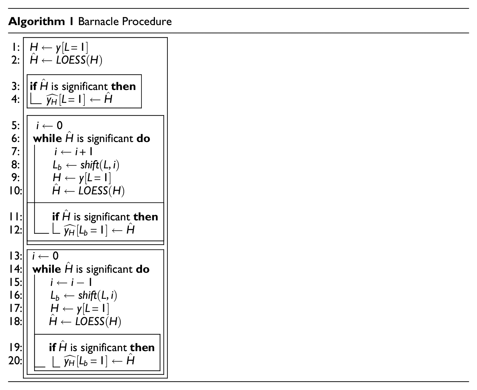
3.4.1. The Barnacle Procedure
While some holidays, such as Ramadan, last several days, others, like Easter, do not. However, this does not mean that their effect is limited only to the “official” holiday dates. To address this spillover issue, we developed the Barnacle procedure. The Barnacle procedure allows us to handle days that are significantly affected by their proximity to a major holiday. We conduct the Barnacle procedure by checking the days adjacent to the holiday for significance. If these days are significant, the subsequent day is checked, and so on, up to a hard limit of forty-six days before and after each holiday. As volatility of the series that observe holiday effects tends to increase around holiday dates, we use an adjusted confidence interval aCI to perform the significance test, Appendix A.4.1. This approach differs from the impact models (constant impact, linear ramp-up and down), used, for example, in Ladiray et al. (2018), as here the shape of the impact is more flexible.
Notation:
3.5. Point-in-Time Seasonal Trend Decomposition with STAHL
Seasonal adjustment methods such as X11 and STL typically employ symmetrical filters to produce high-quality estimates of trend-cycle and seasonal components. However, these approaches may suffer from revisions and forward-looking bias when applied to the most recent observations, which are crucial for timely decision-making. This bias occurs because symmetrical filters use both past and future data points, which are not available at each latest observations in real time. Point-in-time estimates offer an alternative by incorporating only the information available at the time of the publication, eliminating this forward-looking bias.
This methodology is particularly valuable in the context of real-time analysis, where timely and the most accurate, albeit imperfect, information is essential for decision-makers. For instance, it applies to real-time estimation of seasonally adjusted sales for corporations or nowcasting growth, inflation or employment by central bankers and investment managers. Any researchers aiming to simulate decisions as if they were taken in “real-time” may use such adjusted data based upon asymmetric filters. When backtesting trading strategies for example, a forward looking seasonal adjustment methodology will reveal data that is not available to the market participants at the time.
At Quantcube, all series are produced and delivered on a daily basis and cannot be revised. To ensure that the structure of each series remains consistent, the historical parts of each series must be calculated in pseudo-real-time. For a given time series, from the end of the burn-in period to
While symmetrical filters provide more stable and accurate estimates for historical data, point-in-time methods excel in capturing the most current economic conditions without introducing future information. STAHL can leverage the strengths of both approaches: using either symmetrical filters for historical analysis or point-in-time estimates for the most recent observations. Anyone unsure of why the asymmetric version is important or why it should be used can always use the symmetric version.
3.5.1. Asymmetric LOESS
In the classical STL procedure, there are three different stages where forward-looking bias can occur. The first and most obvious is during any step of the LOESS regressions. The second occurs during the low-pass filtering stage, when a moving average is applied in both directions. Finally, during the outlier detection, the median value that is normally calculated using the entire dataset can introduce a bias. To ensure reproducibility and facilitate automation in the generation of time series, these issues need to be addressed.
As a kernel regression, the LOESS applies a weight to the points on each side next to the estimation point. It also applies a non-zero weight to the points in the future. We get around this problem by applying an asymmetric kernel-regression.
The LOESS regression differs from a more classical kernel regression in the way the kernel width is set. In a classical kernel regression the bandwidth is set to a fixed width and the number of points used to make an estimate changes depending on how many data points are present around the estimation point. In the LOESS regression the number of points are fixed and the width of the kernel is set so that the same number of points are always present.
Starting with a kernel width of zero, in regular symmetric LOESS the kernel width is slowly expanded in either direction until the required number of data points is in the bandwidth. In the case of an asymmetric kernel, only the left hand side bandwidth is expanded while the right hand side of the estimation point has a bandwidth of zero.
Mathematically the kernel weighting function differs only slightly from the symmetric kernel. The difference is that is with the asymmetric kernel only the points on the left of the evaluation point are evaluated. With only left hand points adding to the count of
In the edge-case, at the beginning or end of the dataset, the bandwidth can only expand in one direction. Therefore both the symmetric and asymmetric LOESS have identical kernels at the start and at the end. At the start this means that there is a slight phase shift comparing the kernels at the end in Figure 2 makes it clear how the asymmetric kernel replicates the point-in-time estimation of a symmetric LOESS. From this it follows that if the kernel width is set to be the length of the data, the asymmetric kernel will behave exactly the same as the symmetric one.
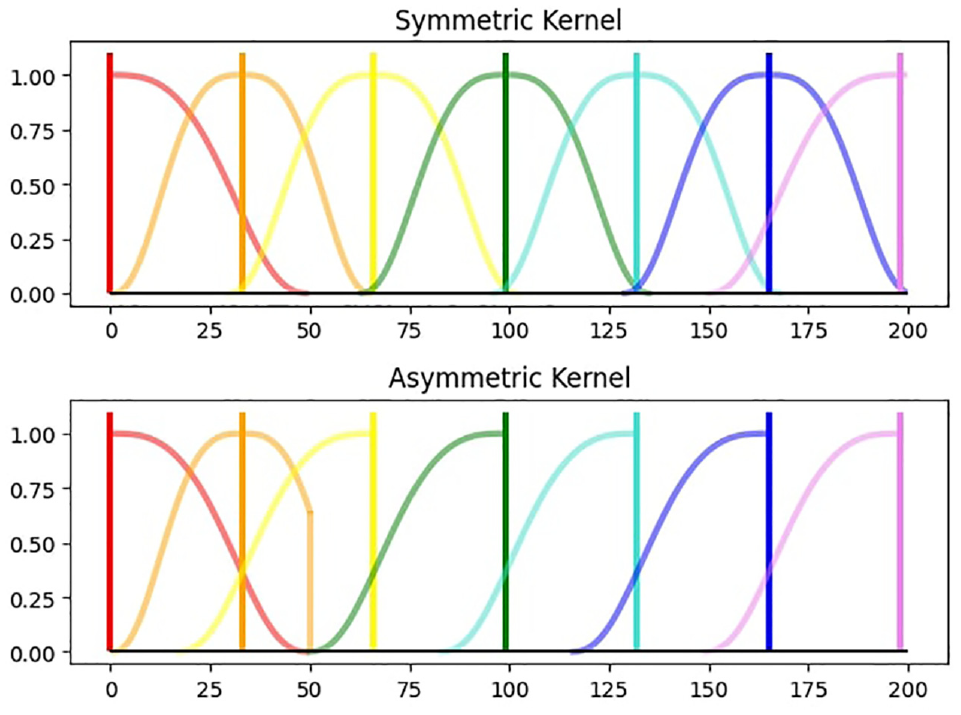
Kernel comparison.
The LOESS asymmetric filter may not be the most optimal filter in terms of gain and phase shift. Grun-Rehomme et al. (2018) provide a comprehensive survey of optimal asymmetric filters and propose an approach that balances the moving average properties in terms of accuracy, revisions and timeliness and allows constructing asymmetric moving averages that present almost no phase-shift. Their work also suggests exploring the non-parametric approach based on spectral theory, as promoted by Wildi (2007), Wildi and McElroy (2016, 2019) with the Dynamic Asymmetric Filters family. This procedure, designed in the frequency domain, would allow the splitting of the revision criterion into two distinct effects, one related to the gain and the other to the phase of the transfer functions. We leave the exploration of introducing alternative asymmetric filters into STAHL for further research.
3.5.2. Extrapolating Moving Averages Procedure
In the STL procedure, the smoothed subseries for the days is extended to be two values longer than the original subseries. The outermost values are determined using linear extrapolation. This ensures that when the bidirectional moving averages procedure is applied, the final series has a length equal to that of the original series. However, an issue arises in that the reverse moving average (MA) procedure uses values from the future. To circumvent this issue, instead of using the smoothed subseries values directly, at each point-in-time, the future values are linearly extrapolated. Then, the moving average procedure is applied to these extrapolated values.
3.5.3. Outlier Weighting
During the outlier weighting, all values are divided by six times the median value of the absolute series. If the entire series is taken into account, this can be considered forward-looking behavior. To prevent this, we set a validation date, so that only the median of the series up to the validation date is considered. This approach ensures that the values of the series do not change when more values are added in the future.
3.5.4. Critical Burn-In Period
The critical burn-in period corresponds to the time span at the beginning of the estimation, during which we are not yet able to produce data in pseudo-real time. Each of the three sources of forward-looking bias has a different burn-in period and affects the structure of the data-generating process in a unique way.
During the early stages of the asymmetric LOESS the kernel start of with a right-tail, then it becomes symmetric before finally reaching its desired left-tailed shape. The LOESS is used in the subseries, the low-pass and the trend. The final LOESS to reach the left tailed shape is the LOESS subseries. This occurs at the point
The extrapolating moving average needs at least two values before it can start extrapolating. As it extrapolated from the same point in each cycle it requires
Finally, the validation date can be set freely and does not significantly impact the seasonal extraction process. It therefore makes sense to set it to be at least
3.5.5. Multiple Seasonality
The STAHL procedure handles the seasonality in an iterative manner, similar to Ollech (2021), and MSTL in Bandara et al. (2021), starting by removing the seasonality of highest frequency first and then moving on to lower frequencies.
3.6. Software
The STAHL procedure takes the form of an internal Quantcube Technology Python library. The preprocessing and seasonality identification steps are handled by Python 3 scripts, using the Scipy (Virtanen et al. 2020) library for Fast Fourier Transform as well as statistical testing. The LOESS filters, as well as the cross-validation procedure, are coded in C for faster performance and then wrapped in a Cython function so that they can be used in the Python environment.
4. Simulation Study
4.1. Construction of Simulated Data
We use simulated series to compare the performance of our model against the current state-of-the-art seasonal adjustment methods. The simulated series are constructed from their subcomponents. Since we know the true values of the components, we are able to evaluate how accurately the methods fit these.
We have chosen TRAMO-SEATS as the benchmark competitor model. TRAMO-SEATS was selected as it is the most commonly used package we could find that closely fulfills the same basic requirements as our method, meaning daily seasonal adjustment as well as holiday adjustment. We test both methods on the series with holiday effects and without holiday effects.
When performing seasonal adjustment on real data, the true subcomponents cannot be directly observed. Holiday and seasonal components can have interacting effects, and the separation between the trend and idiosyncratic components depends on the size of the trend kernel (the
To ensure an exhaustive range of plausible scenarios, we construct 1,000 simulated series. All seasonal effects have a length of 365.24225 days, accounting for leap years. These series incorporate slightly different specifications to test and demonstrate the performance of the methods across a variety of conditions. The specifications we vary include: the length of the series, the variance and shape of the seasonal effect, and the magnitude of the holiday effect. In order to create the final series that is given to the models to be decomposed, we simply add the subcomponents together.
4.1.1. Length
All series are simulated against real dates, beginning on January 1st, 1969. The lengths of these series are uniformly distributed, ranging from 2,000 to 15,000 days. This means each series is between about 5.5 and 41 years years long. Generally seasonal adjustment is not recommended for series shorter than five years. Forty-one years is close to the upper end of currently available daily time series that can be found in practice. The number of days for series

4.1.2. Trend Component
The trend subcomponent is kept very simple. The value of the trend component for a day

4.1.3. Seasonal Component
The seasonal component varies both in variance and in shape. Seasonal effects can exhibit very different patterns. To cover a large spectrum of possible seasonal patterns we use four different equations. Each equation has an equal chance to be applied to the series. All seasonal components are first normalized to have a mean equal to zero. The standard deviation of the seasonal component is then randomly set from a uniform distribution between 1 and 5 (
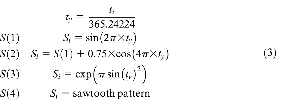
Plots of these can be found in Appendix A.5.
4.1.4. Holiday Component
For the holiday component we chose to focus on simulating one moving holiday. We selected to simulate Easter because it is a holiday that is known to have real world effects and that is a proper moving holiday. The holiday effect is zero for most of the year. We allow the Easter holiday effect to start to ramp up ten days before and to ramp down five days after Easter. For each series the baseline holiday effect for Easter is set between 1 and 7. On top of that, for each individual holiday occurrences an additional noise value is sampled from a Gaussian distribution with a standard deviation of 0.5. When we test the methods (STL or TRAMO-SEATS) without holiday effects, we don’t include the holiday component. When we test STAHL or TRAMO-SEATS-H we include the holiday component in the input series.
4.2. Evaluating the Optimal H Discounting Value
We use the simulations to gain a better understanding of how to set the H discount value. This value ensures that the methodology can handle both seasonal and holiday effects simultaneously. It achieves this by discounting the holiday effect before the start of the STL inner loop. This ensures that the seasonal component retains a significant proportion of the total variance relative to the holiday component.
We evaluate the optimal H discount value by examining the RMSE of the estimated holiday component. To determine the optimal H discount value, we try values between 0.1 and 0.9. Fitting a quadratic curve through the observed values, we find that the approximate optimal value is just under 0.5 and is set to be 0.5 in the model. The results in terms of RMSE for the holiday and barnacle days are shown in Figure 3 below. If we subtract the holiday component from the raw series without a discount value and the holiday effect is overestimated for one or more occurrences, the STL inner loop will try to compensate the overestimation. This can lead to a cascading effect where the two components work in opposite directions. The H discount value works as a regularization technique to counteract this phenomenon.
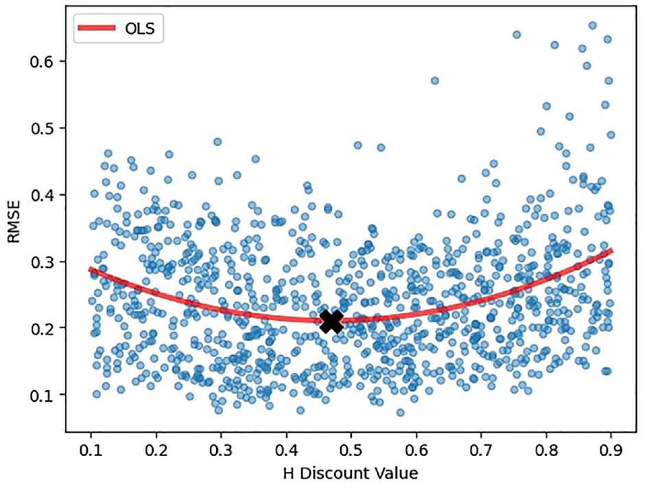
Optimal H discount value.
4.3. Comparison to TRAMO-SEATS
To evaluate the different strengths and qualities of the seasonal extraction methods we look at several different test. TRAMO-SEATS does not have a pseudo-real time feature, so we will compare it primarily to the symmetric version of STL and STAHL. In order to illustrate the secondary contribution of this paper we will also compare it to the pseudo real-time STL and STAHL models that use asymmetric kernels. We will refer to these as ASY-STL and ASY-STAHL for this section of the paper.
We use the fractional Airline Estimation of TRAMO-SEATS. We add Easter as the only holiday.
It is very important to note at this point that when examining the asymmetric versions of STL and STAHL, these asymmetric versions introduce distinct modifications to their respective base algorithms, rendering a direct, one-to-one comparison methodologically unsound. The regular STL and STAHL procedures use a kernel that is the entire length of the data set. If we did the same with the asymmetric version, then they would not be asymmetric (this is explained in Subsection 3.5). We therefore use a kernel that is only 75% the length of the dataset. We do this to prove that the methodology works to quickly provide pseudo-live estimates. We would always suggest to use the symmetric versions of STL and STAHL if pseudo-live estimations are not required. As many clients of QuantCube are active in financial markets and need to backtest trading strategies, this approach is necessary in this particular case.
We start off looking at how well TRAMO, STL and ASY-STL deal with their primary tasks: seasonal adjustment. We then move on to look at the primary contribution of this paper which is the holiday extraction. Each model is asked to remove holiday effects from a series, including barnacle days. When we ask TRAMO-SEATS to extract holiday effect estimates we refer to it as TRAMO-H or TRAMO-SEATS-H.
For the first approach, we use a spectral density analysis to examine if there is still seasonality in the seasonally adjusted series. We also use a QS-test16 to relativize how much of the seasonality has been removed.
When examining the subcomponents, we check for residual seasonality in the idiosyncratic component and the trend. We also check the RMSE and correlation between the simulated and estimated subcomponents.
We perform an F-test to examine if the holiday dates, and the holiday dates combined with the barnacle dates, have a significant effect.
4.3.1. Spectral Analysis of Seasonally Adjusted Series
The spectral density plot of the seasonally adjusted series is analyzed to examine whether there is a peak at the one-year mark.
A peak would indicate that the series still contains some seasonal variance, meaning that there is residual seasonality. The results can be seen in Table 1.
Seasonal Detection Out of 1,000 Series.
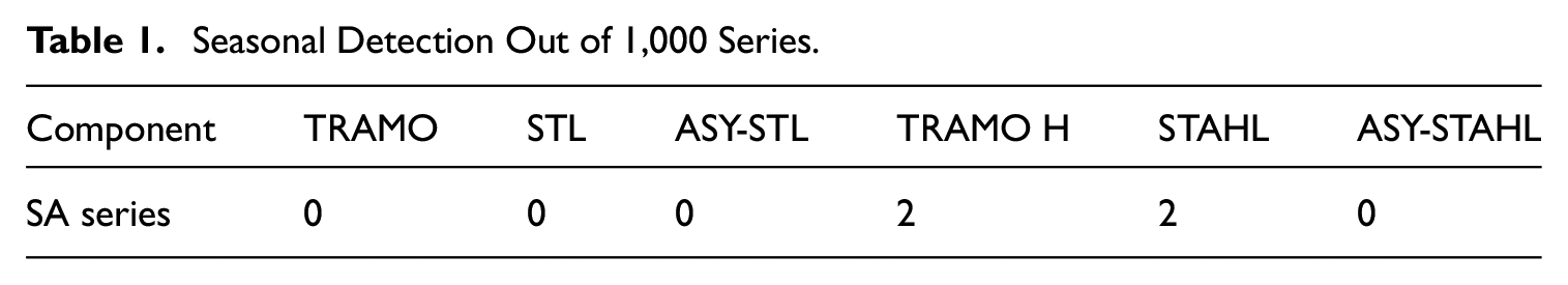
Out of 1,000 series, we detect seasonality two times for both TRAMO-H and STAHL and never for any of the other series. We examine more closely the seasonally adjusted pattern of one of the series where both methods failed (Figure 4) and plot also the ASY-STAHL estimate for this occurrence, even though the spectral density test has not detected any seasonality. The level of the series have been changed so they can be seen individually. We observe that the remaining seasonality comes from the imperfectly estimated Easter effects. There is a distinct bump in the TRAMO-H series, more clearly visible than in the other two series. The spectral density test does not identify any seasonality in the ASY-STAHL because the
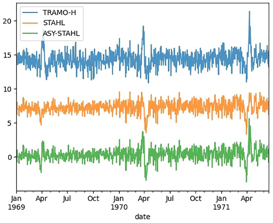
Seasonally adjusted series with residual seasonality (level changed to aid visibility).
Upon visual inspection, it becomes evident that both methodologies effectively remove the seasonal component from the series. The residual seasonality is, in fact, a result of improperly estimated holiday effects. In this instance, we contend that the STAHL methodology demonstrates a superior performance, particularly with less pronounced residual holiday effects.
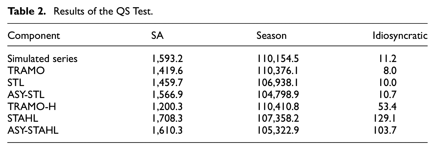
4.3.2. QS-Test
The QS-test is an adapted Ljung-Box test, computed on the seasonal lags. We compute the QS statistics on the seasonally adjusted series (SA), the seasonal and the idiosyncratic components produced by each methodology, as well as on the “true” components in the simulated series. The idea is to use the QS statistics as a metric to quantify the seasonality in each component, and compare it with the seasonality of the components in the simulated series. We compare the results (Table 2) of the methodologies to those from the simulated series. Our findings indicate that both the STL and TRAMO-SEATS approaches yield results very similar to the original series, suggesting both effective seasonal adjustment and accurate component separation. When addressing holiday effects, both methods exhibit slight imperfections in their decompositions. Regarding seasonal adjustment both methods perform relatively well: while TRAMO-SEATS records lower QS statistics for the seasonally adjusted series, STAHL produces results more closely resembling those of the original simulated series. Encouragingly, we can see that the results of the asymmetric STL and STAHL implementations do not vary very much from the symmetric versions.
Results of the QS Test.
4.3.3. RMSE
The RMSE is computed between each component (seasonally adjusted, seasonal, trend, idiosyncratic) produced by the different methodologies and their respective “true” component from the simulated series (Table 3). The RMSE analysis reveals that TRAMO-SEATS demonstrates superior accuracy in decomposing the series. Notably, we observe that this performance differential diminishes as the length of the series increases. The STL methodology clearly relies more on having a large enough dataset than TRAMO-SEATS does.
RMSE.
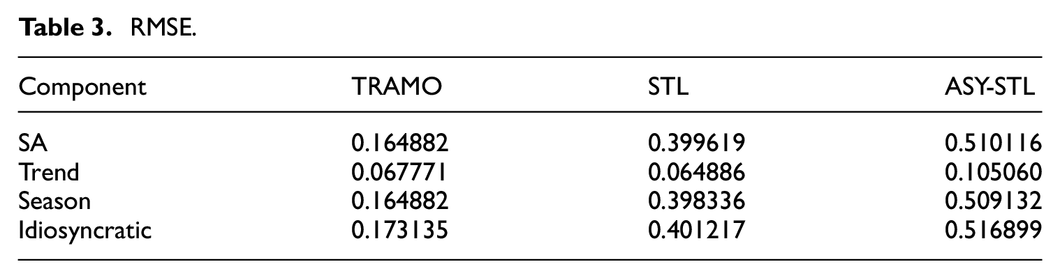
Upon examining the additional RMSE plots and the differences between the TRAMO-SEATS and STL seasonally adjusted series and seasonal components, we propose that the STL output might benefit from an additional level of smoothing. The plots in Appendix A.6 demonstrate that STL and TRAMO-SEATS perform similarly in this regard.
When analyzing the results of series with holiday effects, we observe that the differences between TRAMO-SEATS-H and STAHL are minimal (Table 4). It is evident that the TRAMO-SEATS methodology is relatively more affected by the presence of holidays.
RMSE with Holiday.
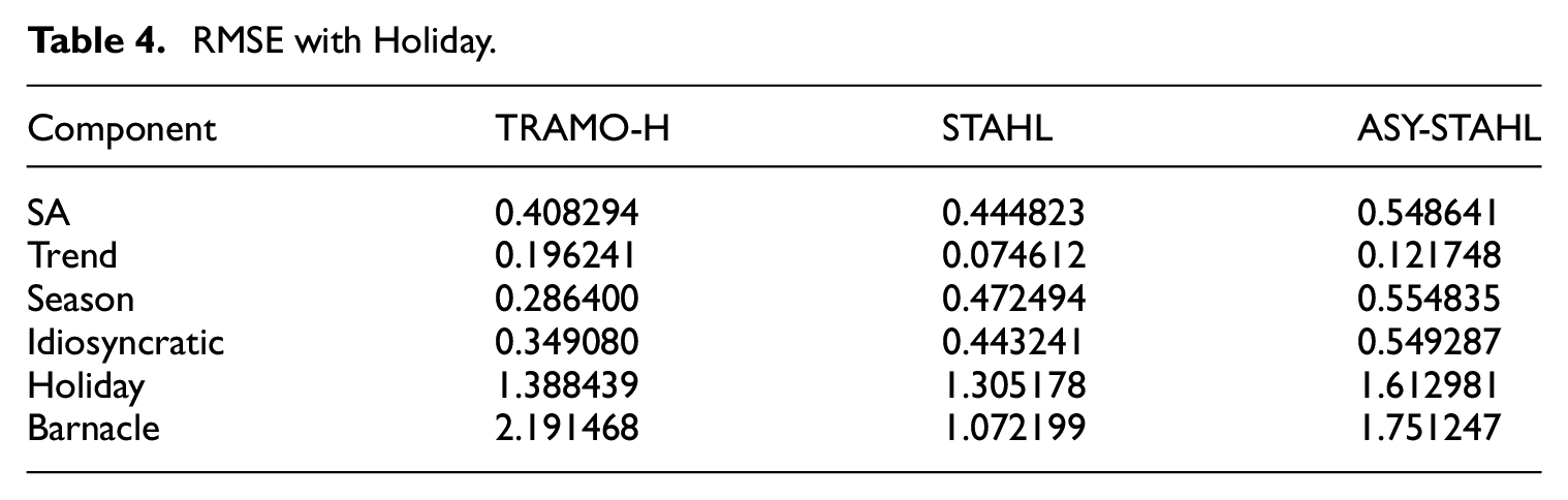
As illustrated in Figure 5, while TRAMO-SEATS-H outperforms STAHL in shorter series, this performance differential diminishes in longer series. Figure 6 demonstrates that even as series lengths increase, the quality of TRAMO-SEATS’ estimation of the holiday component does not improve commensurately. These observations suggest that TRAMO-SEATS encounters greater difficulties in handling the holiday effect, particularly with respect to the barnacle days accompanying the holidays.
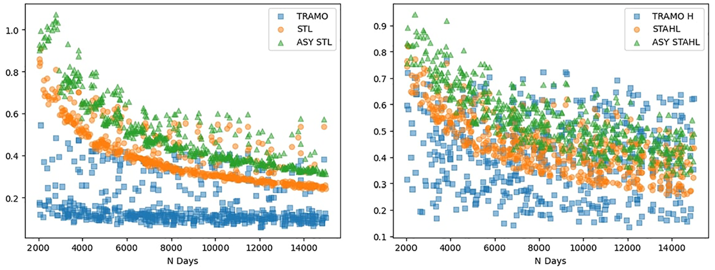
RMSE of seasonally adjusted series.
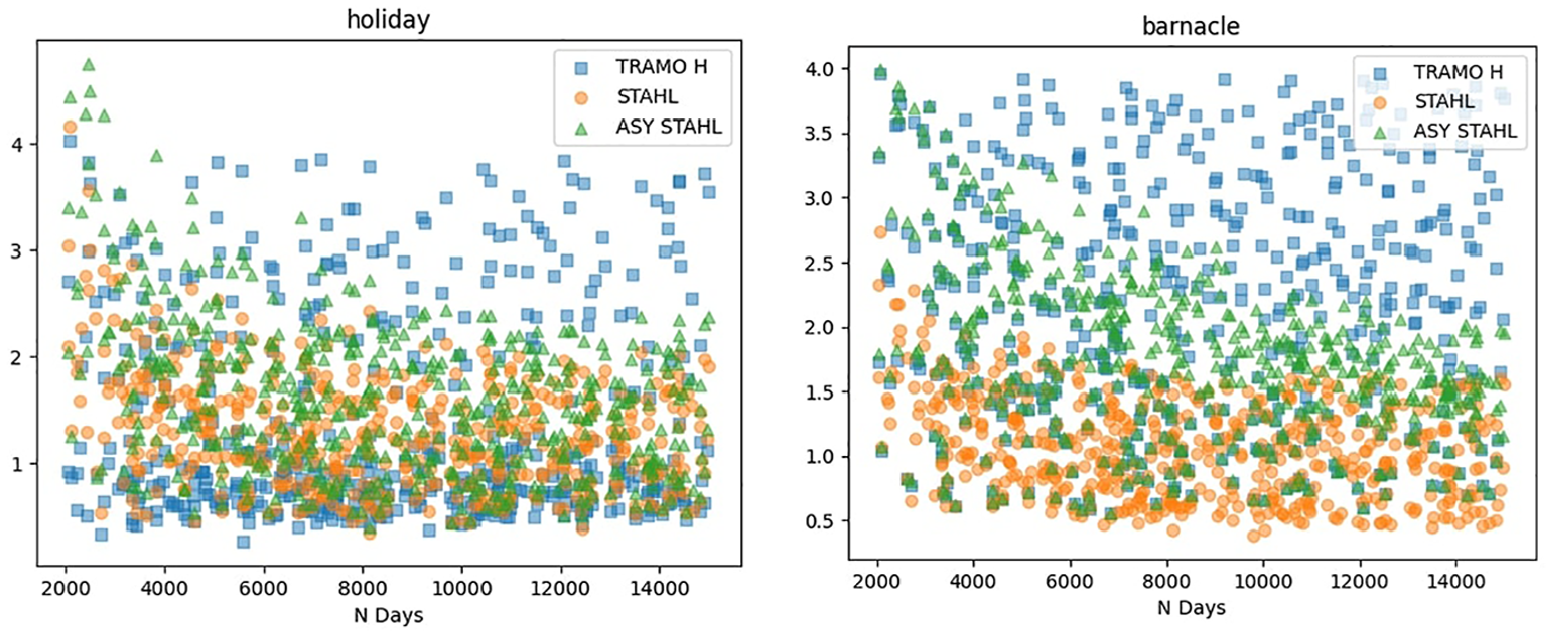
RMSE on holiday and barnacle dates, X = N Days.
The size of the holiday effect is on the x-axis of Figure 7. The simulated holiday size is between 1 and 7. We observe that the TRAMO-SEATS does a relatively good job with smaller holiday effects but really starts to struggle when the holiday effect goes above 5. In addition, STAHL demonstrates superior performance in handling barnacle days across all holiday effect magnitudes.
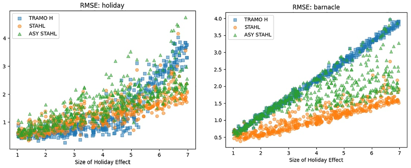
RMSE on holiday and barnacle dates, X = holiday effect size.
From Figures 6 and 7 we can deduce that the ASY-STAHL slightly struggles with the barnacle days when the series is not very long or when the size of the holiday effect is not very large. The reason for this is quite simple. As we reach the edge of the Loess the CI increases (Appendix A.4.1). This is because on average the data points are further away. Shorter series and series with fewer significant holiday effects are therefore more likely to reject the significance of the barnacle day.
4.3.4. F-test
The final test we perform is a F-test on the holiday date dummies and the barnacle day dummy (Figure 8). This test confirms our previous results. The STAHL method exhibits outstanding efficiency in managing both holiday effects and barnacle days in time series data. TRAMO-SEATS does well with small holiday effects, but cannot effectively deal with large ones and barnacle days. We notice only a minor loss of performance when going from the symmetric version of STAHL to the asymmetric version. Plots of the p-values are in Appendix A.7.
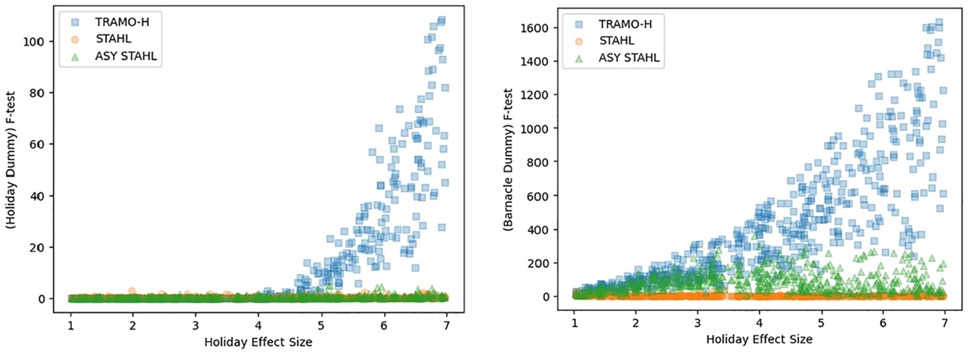
F-test of holiday and barnacle day dummies.
4.3.5. Visual Inspection of Holiday Estimation
While TRAMO-H uses a parametric ARIMA approach to estimating the holiday effect, STAHL uses a much more flexible nonparametric approach. The model is allowed to search for barnacle days on each side of the holiday period. When examining the estimated values for the holiday effects in Figure 9, we can see that TRAMO-H only produces an estimate for the holiday itself. Meanwhile, both STAHL and ASY-STAHL are able to produce estimates for the surrounding barnacle days as well. This leads to the barnacle days being statistically significant when examined with an F-test (Figure 9).
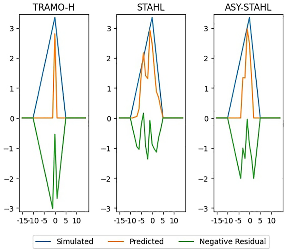
Average (median) holiday estimation.
We sort the holiday estimation by relative RMSE
4.4. Simulation Study Discussion
From the simulation study we can conclude that TRAMO-SEATS outperforms the STL and STAHL methodologies for short time series. This discrepancy decreases with increasing series length. When holiday effects are introduced STAHL seems to have an edge at integrating them into the subcomponent estimation.
Our observations clearly demonstrate the efficacy of the Barnacle procedure, introduced in this paper, in addressing leading and lagging holiday effects. Given its effectiveness, further research could explore the potential incorporation of this procedure into other methodologies, potentially expanding its applicability and impact in the field of time series analysis.
5. Empirical Illustrations
5.1. Traditional Weekly Data: US Initial Unemployment Insurance Claims
5.1.1. Data Description
As a first example, we applied the STAHL procedure to the US Initial Unemployment Claims series. This weekly series, published by the US Employment and Training Administration, covers the number of initial unemployment claims made by unemployed US individuals to be eligible for employment benefits. It is published both as a seasonally adjusted and a non-seasonally adjusted series every Wednesday. This series is relevant to illustrate our seasonal adjustment procedure for the following reasons:
Its weekly frequency allows us to illustrate the resampling procedure.
It exhibits outliers that can be due to catastrophic external events (hurricanes, the Covid pandemic outbreak) or labor-related events (strikes).
It is a relevant series for tracking the macroeconomic situation and the business cycle, used, for instance, in high-frequency composite indicators such as the Aruoba-Diebold-Scotti Business Conditions Index.
5.1.2. Official Seasonal Adjustment Methodology
The official initial claims seasonal adjustment is performed by the Bureau of Labor Statistics (BLS) and has relied on the methodology described in W. P. Cleveland et al. (2014) since 2002. The series exhibits yearly multiplicative and the seasonal factors are computed using a locally weighted regression on sine and cosine terms, with the weights extracted from a state-space modeling of the series. There is no trend extraction per se, as the series are detrended by differentiating before the seasonal adjustment. The holiday procedure is based on the X-13-ARIMA-SEATS program, with holiday weights constant over time. The outliers and intervention adjustment also use the X-13-ARIMA-SEATS program.
The official data both SA and NSA is subject to revisions with each publication. The main source of changes is the revisions of the seasonal factors, as showed in Figure 10. We focus in this illustration on the claims values for the first publication and the last available vintage (end of October 2023).
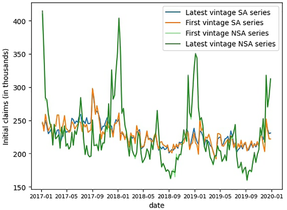
Revisions of the initial claims data, first to last vintage (October 2023).
The Covid-19 pandemic has also led to further changes in the methodology. Due to its extreme impact on unemployment claims, the BLS changed the seasonal factors from multiplicative to additive for the period from March 2020 to June 2021, then switched back to multiplicative after that date. The extreme nature of the event and its duration also necessitated an a posteriori update (in April 2023) of the outliers’ specification during the pandemic period, leading to major revisions of the seasonal factors from the end of 2021.
5.1.3. STAHL Set-Up
We will now apply the STAHL procedure to produce our own version of the seasonally adjusted claims data. In doing so, we are operating under real-time conditions, meaning that there are no revisions of the data, and we use real-time data vintages from May 2009 to November 2023.
First, following the official procedure, we assume a multiplicative seasonality scheme, meaning a log transformation is applied. Given the weekly frequency of the data, we apply the resampling procedures described in Subsection 3.1.2 to have 53 equally spaced datapoints per year. The resampled holidays given to the HTL procedure are the following: New Year’s Day, Washington’s Birthday, Memorial Day, Independence Day, Labor Day, Columbus Day, Veteran’s Day, Thanksgiving, Christmas, and Easter. The Barnacle procedure detects barnacle days effect before and after Thanksgiving and Independence day.
During the Covid period, we do not make the switch to additive, and keep the multiplicative scheme. However, even with the built-in robustness to outlier of the STAHL procedure, the unprecedented extreme behavior of the series during that period contaminates the seasonal adjustment for the years 2022 and 2023. Therefore on that front we follow the BLS choice, and remove the period from March 2020 to June 2021 from the data when performing STAHL starting January 2022.
5.1.4. Point-in-Time Seasonal Adjustment with STAHL
We observe in Figure 11 that the seasonal adjustment obtained via STAHL follows closely the official seasonally adjusted signal, both in terms of trend and idiosyncratic behavior. The procedure is robust to outliers. For instance, the amplitude of the peak in August 2017 due to hurricane Harvey matches the one measured in official data. However, the volatility around the Thanksgiving period is higher for our model than for the official data, a consequence of the upsampling.
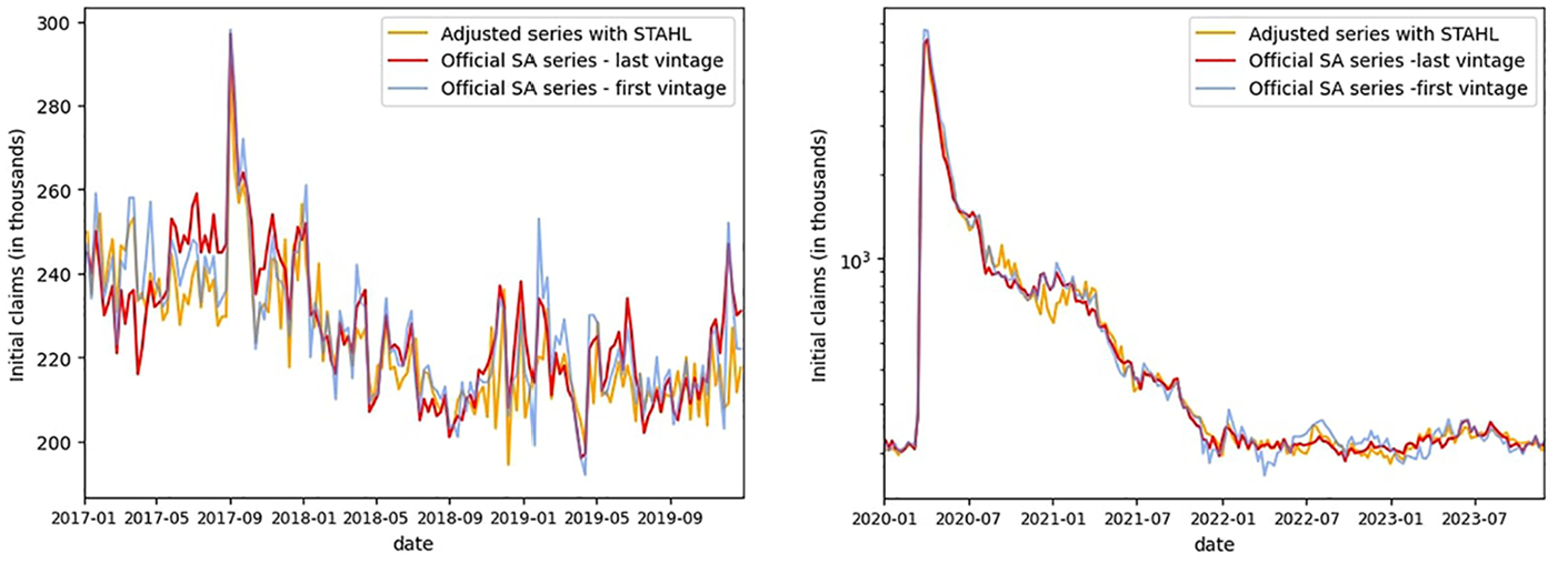
Comparison of STAHL versus first and last vintage SA (before [left] and after [right] the Covid period).
Regarding the Covid period, as observed in Figure 11, STAHL is sufficiently robust to outliers, such that maintaining a multiplicative scheme yields results similar to those of the BLS methodology for the period from April 2020 to December 2021. However, it is noteworthy that STAHL output diverges from the official data briefly in January 2021, before recovering. For the post-Covid period, the real-time output of STAHL is less volatile than the first estimates and closer to the latest vintage. This illustrates both the stability of our model over time and the benefit of hindsight gained from excluding the Covid period starting in 2022.
A visual analysis of the spectral density for the non-seasonally adjusted original series and the STAHL seasonally adjusted series (see Figure A6 in Appendix A.9) shows that the procedure removes all the seasonal peaks from the spectrum while preserving the lower frequency components. The metrics shown in Table 5 confirm that, in the post-Covid period, the STAHL model is closer to the latest estimates than to the first vintage in terms of Mean Absolute Log Difference (MALD). In the pre-Covid period, the Mean Log Difference (MLD) of STAHL compared to both the first and last vintages is close to
Median Log Difference and Median Absolute Log Difference of STAHL Compared to Official Data.
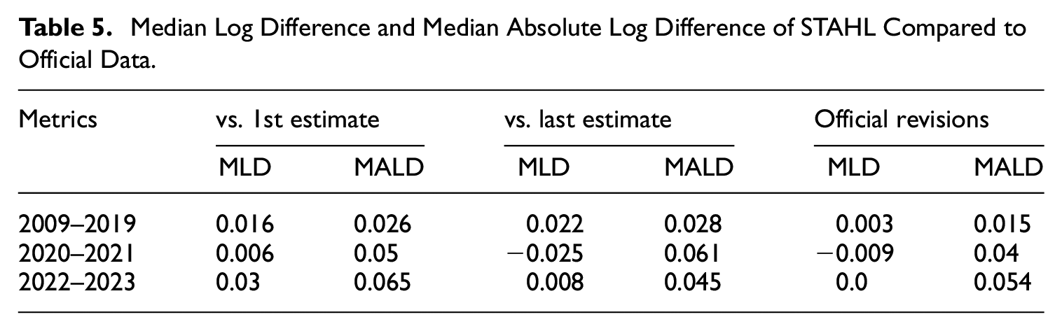
Through this illustration, we demonstrate the capacity of STAHL to reproduce the seasonal adjustment of the official methodology for high frequency data using a robust, more parsimonious, and purely point-in-time method.
5.2. Holiday Adjustment: Google Searches for “Easter Bunny”
5.2.1. Data Description
Easter is a tricky holiday to capture in a seasonal adjustment procedure, as it does not have a fixed place in the Gregorian calendar. To illustrate its effect, we chose the Google Search Volume series for the keywords “Easter Bunny.” While most series have both seasonal and holiday effects, this series has been specifically selected because all movements can clearly and easily be attributed solely to the holiday effect. It therefore serves as an excellent test bed to demonstrate the issues that can arise when trying to adjust for holidays using the standard STL procedure, which is conceptualized for regular seasonal effects. The Google Search Volume series starts in 2010 and goes all the way to August of 2023, comprising 4,981 daily values. They range between 0 and 100, with the values representing the relative search volume for the period.
5.2.2. Applying Classical STL
When we look at the first 500 days of the Easter Bunny Google searches in Figure 12, two of the Easter events can be easily isolated. The uptick in searches starts quite some time before Easter and then quickly drops once Easter is over. Here, we illustrate the consequences of applying STL-based seasonal adjustment to the Easter Bunny series. Since the temporal pattern of Easter Bunny searches is governed by the variable date of the Easter holiday rather than the fixed calendar date, this approach is methodologically inappropriate.
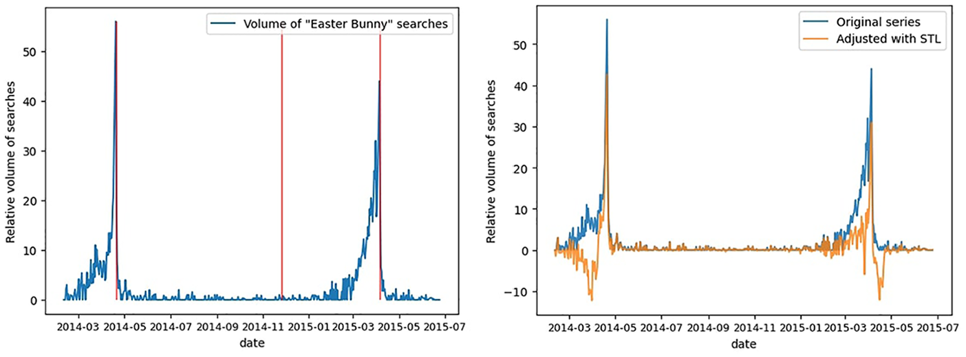
Easter Bunny searches: original series and seasonal adjustment with STL.
Examining the same time period after having seasonally adjusted the series using the classical STL approach (Figure 12), the results appear rather disappointing. For each of the two Easter events, STL assigns some negative values: for the first day before Easter, and for the second day after Easter. Clearly, the fact that Easter moves around confuses the STL procedure, which tries to find some kind of “average” Easter effect over a longer time period.
5.2.3. Applying HTL
As it is obvious that the classical STL procedure is not well-suited to handle moving holiday effects, we developed the HTL procedure. Conceptually, HTL works in a very similar way to the STL procedure. The main difference lies in the fact that the subseries consist only of the holiday events, rather than having a subseries for every period in a seasonal cycle.
Figure 13 shows the estimated holiday effect for Easter alongside the original series. While Easter is deemed significant (and thus an “Easter effect” is estimated), the results are not very impressive. The estimated Easter effect appears much smaller than the actual effect and is confined to only one day per Easter event. To correct for this, we developed the Barnacle procedure (see Appendix). In the Barnacle procedure, we begin by testing the statistical significance of the holiday effect. If the holiday is found to be significant, we repeat the process with the days on either side of the holiday, that is, the barnacle days. We continue this process until we reach a day that is not significant or we reach the 46-day limit.
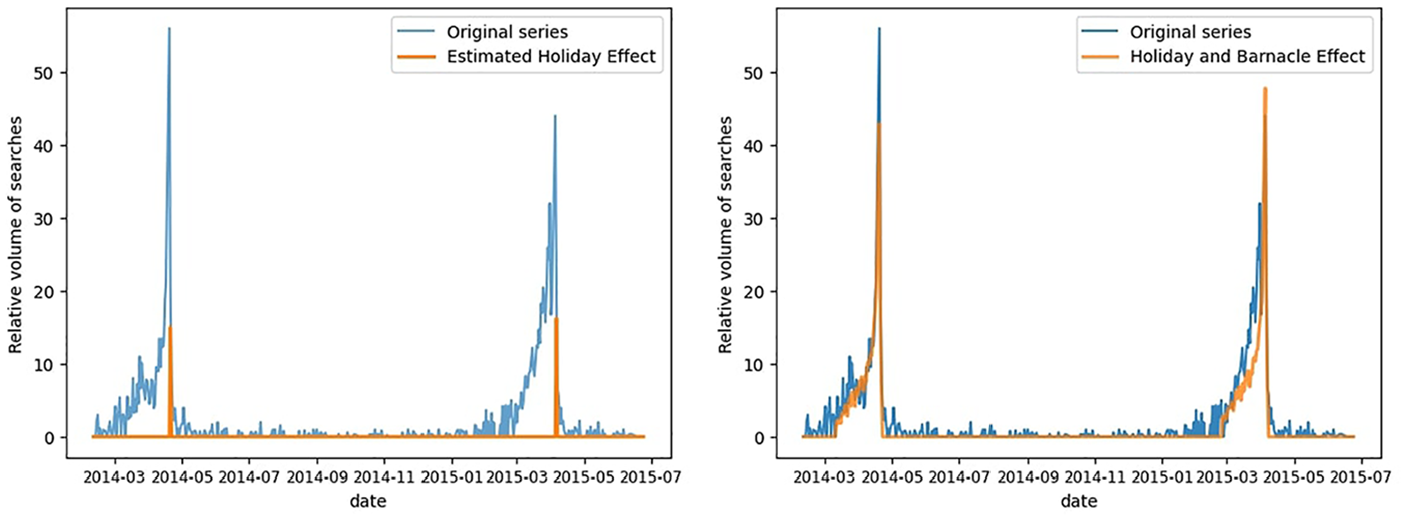
Easter Bunny searches and estimated holiday effect: without barnacle effect (left) and with (right).
In Figure 13, we can see that once we include the barnacle day effects our estimations are much closer to the original series than before. Figure 14 illustrates the dramatic improvement that comes from switching from STL to HTL with the Barnacle procedure. As such, we are able to reduce both the positive and the negative extremes of the series.
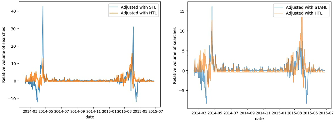
Adjusted series for “Easter Bunny” searches using HTL versus using STL (left), and using HTL versus STAHL (right).
We clearly demonstrate that for series where the effect depends mostly or entirely on holiday dates, and can have leading/lagging effects; classical seasonal adjustment techniques will not work. The HTL approach is particularly effective here because it is able to center the effect around the moving Easter date, as well as accounting for the leading effects that we observe in this series. The nonparametric Barnacle approach to finding the number of leading/lagging days differs fundamentally from the fixed approaches to holiday adjustment used by X-13.
5.2.4. STAHL Application of Easter Bunny Searches
This series of searches for the Easter Bunny is simpler than many other series that Quantcube uses daily. The main difference is that this series exhibits purely holiday effects, whereas most series have a mix of holiday and seasonal effects. We will examine this in more detail in the next section. Figure 14 demonstrates the seasonally adjusted series using HTL and STAHL. We can observe that the STAHL seasonal adjustment slightly struggles with the negative effects, similar to what we observed in the STL procedure. However, it is also evident that STAHL can handle the dates close to the Easter event quite effectively. The efficiency of the HTL adjustment is visually confirmed by the spectral density graph (see Appendix A.9, Figure A7), where we observe that the HTL procedure removes the quick succession of peaks present in the density of the non-seasonally adjusted (NSA) data. These peaks correspond to the Fourier transform of a Dirac comb-like holiday pattern.
5.2.5. Negative Output Values
The number of Google searches can obviously not reach negative values. The STAHL procedure is not explicitly developed to deal with strictly positive values so we leave the results as they are to demonstrate to the reader how the methodology functions, without additional steps muddying the waters. In practice we would set a minimum value of zero to ensure strict positivity. For some series it can be worthwhile to seasonally adjust the log-values and then use the exponential of the seasonally-adjusted log series to maintain strict positivity. When examining the results in Figure 14 we can see that one of large advantage of the HTL procedure is that it produces significantly less negative outputs than STL or even STAHL.
6. Conclusion
In this research note, we unveil STAHL (Seasonal, Trend, And Holiday decomposition based on LOESS), an innovative framework for seasonal adjustment developed by Quantcube Technology. Drawing on the STL method pioneered by R. B. Cleveland et al. (1990), STAHL has been specifically crafted to accommodate the intricate seasonal patterns observed in diverse daily datasets, such as satellite imagery, textual analytics, daily pricing records, or web searches. STAHL’s utility is manifold, but its three primary enhancements stand out.
A key feature is the “holiday-loop” algorithm, which efficiently handles time-varying calendar effects, including diverse holidays such as the Chinese New Year and those following the Hijri calendar. The Barnacle procedure extends this capability, addressing not only the direct impact of holidays but also their anticipatory and lingering effects.
Additionally, we introduce the asymmetric kernel to produce point-in-time estimation, which significantly enriches the “systematic production” of seasonally adjusted series. This advancement paves the way for subsequent exploratory research into various asymmetric filters to potentially improve the point-in-time trend extraction procedure. Lastly, STAHL’s enhanced capability for handling missing values represents a leap forward in robustness, facilitating the management of gaps in seasonal data.
The practical applications of STAHL have been thoroughly tested, showcasing its ability to proficiently produce data that is adjusted for both seasonal and holiday effects across a spectrum of frequencies and series types, including both traditional and non-traditional ones. This establishes a new benchmark for automated seasonal adjustment of large scale high frequency datasets and may broaden the horizon for future applications in this domain.