
Abstract
Both the ongoing digital transformation in many statistical agencies around the world and the COVID-19 pandemic outbreak in 2020 have increased the recognition of and demand for infra-monthly economic time series in official statistics during the past decade. Infra-monthly data often display complex forms of seasonality, such as superimposed seasonal patterns with potentially fractional periodicities, that prevent the application of traditional modeling and seasonal adjustment approaches. For that reason, JDemetra+, the official software for harmonized seasonal adjustments of monthly and quarterly data in Europe, has been augmented recently with several methods tailored to the specifics of infra-monthly data. This includes a modified TRAMO-like routine for data pretreatment and extended versions of the ARIMA model-based and X-11 seasonal adjustment approaches alongside the classic STL method. These methods can be accessed through either the graphical user interface or an R package suite, which also provides additional routines for structural time series modeling. We give a comprehensive description of all those methods and discuss the theoretical properties of their key modifications. Selected capabilities are then illustrated using daily births in France, hourly realized electricity consumption in Germany, and weekly initial claims for unemployment insurance in the United States.
Keywords
1. Motivation
Many macroeconomic time series compiled and published by statistical agencies at regular sub-annual intervals display seasonal fluctuations, that is, movements that recur each year in the same season with similar intensity. The presence of such repetitive movements often obscures underlying economic trends and other non-seasonal dynamics that are usually of more interest for the majority of data users. For that reason, seasonal adjustment, that is, the process that seeks to remove seasonal fluctuations from observed time series as best as possible, has been an integral part of data production in official statistics for many decades. Fostering harmonized production processes across statistical agencies, both Eurostat, which is the statistical office of the European Union, and the European Central Bank have recommended JDemetra+ (JD+) as the time series software for conducting seasonal adjustment of official statistics within the European Statistical System and the European System of Central Banks since February 2015 (see Eurostat and European Central Bank 2015). The JD+ program is mainly developed at the National Bank of Belgium in cooperation with the Deutsche Bundesbank and the French National Institute for Statistics (Insee). It implements the popular X-11 and autoregressive integrated moving average (ARIMA) model-based (AMB) seasonal adjustment approaches for monthly and quarterly data under version branch 2.x, including their respective regARIMA and TRAMO time series regression frameworks for data pretreatment (see Grudkowska 2017 and Smyk et al. 2024 for a documentation of JD+).
A new chapter has begun with the inaugural JD+ release from the version branch 3.x in May 2023, as version 3.0 contains generalized modeling and seasonal adjustment methods for time series of any seasonal periodicity. The addition of those methods was primarily motivated by an increasing popularity of and demand for infra-monthly time series in official statistics over the past decade. This evolution has been largely fostered by the emergence of new digital data sources and automated data collection methods that provide easy and sometimes almost real-time access to such data. As a consequence, many statistical agencies have started to explore ways to replace or complement traditional measurement models with new models that are capable of blending survey data with administrative and digital data sources (cf. Jarmin 2019; Radermacher 2019). In 2020, the demand for daily and weekly data soared immediately after the outbreak of the COVID-19 pandemic as many institutional data users asked for more timely indicators to monitor current economic developments, often with the aid of so-called experimental statistics such as dashboards as well as early warning and sentiment indicators (see, e.g., Eraslan and Götz 2021; Keane and Neal 2021; Lewis et al. 2022). Although being strongly seasonal in many cases, infra-monthly economic data do not lend themselves to being modeled with classic Box-Jenkins approaches and seasonally adjusted with traditional methods due to a variety of peculiarities not seen in monthly and quarterly data. Prime examples include the coexistence of multiple seasonal patterns with potentially fractional periodicities, direct measurability of granular calendar variation and a high susceptibility to various forms of irregular variation (see the discussion in Section 2).
In general, there are three possible strategies in official statistics to resolve those issues: first, proper data regularization so that traditional modeling and seasonal adjustment approaches become applicable to the regularized infra-monthly data; second, proper modifications to traditional approaches so that they become applicable to the unaltered infra-monthly data; third, application of proper approaches not considered in official statistics so far. Following the second strategy for the most part, JD+ 3.0 implements a modified TRAMO-like pretreatment routine as well as extended versions of the AMB and X-11 seasonal adjustment approaches. Those methods are accompanied by the classic STL approach that comes without any modification for dealing with fractional periodicities. The corresponding routines have been implemented in Java and can be accessed easily through both the graphical user interface and an R package suite, which also provides additional routines for estimating structural time series models.
The purpose of this paper is to elaborate on the main modifications to the traditional modeling and seasonal adjustment approaches, to give additional theoretical details, and to discuss and illustrate selected properties of the key underlying models and filtering methods. Our target audience consists of both experienced and potentially new JD+ users who wish to find an updated documentation of the software’s current developmental stage, and—more generally—of anyone interested in recent advances in seasonal adjustment methods for infra-monthly data. The latter type of reader is also referred to the broader overviews provided in Evans et al. (2021), Ladiray et al. (2018), and Webel (2022). We start with a brief review of the main characteristics of infra-monthly time series, including the introduction of our baseline unobserved components model (Section 2). We then discuss data pretreatment through a time series regression model in which the residuals follow an Airline-type ARIMA model that allows for multiple first-order seasonal differencing and moving average polynomials as well as fractional powers of the backshift operator (Section 3). The same model is then used to introduce proper modifications to the traditional AMB approach (Section 4). The extended X-11 and classic STL approaches are presented in Sections 5 and 6, respectively, followed by a brief description of structural time series models (Section 7). Selected capabilities of these methods are then illustrated using daily births in France, hourly realized electricity consumption in Germany, and weekly initial claims for unemployment insurance in the United States (Section 8). R code snippets that can be used to rerun these examples are contained in the Supplemental Material. We conclude with some final remarks and suggestions for future developments (Section 9).
2. Infra-Monthly Time Series
2.1. Data Peculiarities
Infra-monthly economic time series often display dynamics that cannot be seen in data recorded at traditional sub-annual intervals, such as months and quarters. Therefore, we briefly summarize their key distinctive features; detailed discussions can be found in de Livera et al. (2011), Ollech (2023), Proietti and Pedregal (2023), and Webel (2022), amongst others.
The seasonal dynamics of infra-monthly time series are typically more complex than those of monthly and quarterly data. The main reason is the potential coexistence of multiple seasonal patterns that can even have fractional periodicities (the origin of this phenomenon is explained in Remark 1 below). To exemplify this increased complexity, Figure 1 shows realized hourly electricity consumption in Germany over the course of April 2023. Both infra-daily and infra-weekly repetitive patterns are clearly visible in this series: electricity consumption is usually lower during nighttime, sharply increases in the morning, peaks around lunchtime, displays a minor dip in the mid-afternoon and eventually decreases until bedtime. This infra-daily pattern can be seen on any given day of the week; however, its average level and wingspan are noticeably smaller on Saturdays and especially on Sundays, creating a characteristic infra-weekly pattern. In addition, a

Realized hourly electricity consumption in Germany in units of gigawatt hours (GWh) from Saturday, April 1, 2023 (00:00 AM) through Sunday, April 30, 2023 (11:00 PM). Gray area marks the Easter period (April 7–10).
Compared with monthly and quarterly data, the calendar-related dynamics of infra-monthly time series are often more complex as well since data granularity enables more accurate measurements of effects related to both fixed and moving holidays, including potential interactions with the seasonal patterns. During Easter 2023, for example, it is seen that hourly electricity consumption exhibits quite peculiar swings on Good Friday and Easter Monday whereas the series displays relatively normal infra-daily and infra-weekly dynamics on Easter Saturday and Easter Sunday (Figure 1). Data granularity also facilitates measurements of anticipatory and catch-up effects as well as of effects of holiday-related events, such as bridging days, which are usually unquantifiable for monthly and quarterly economic time series and hence not recommended for consideration in official seasonal adjustments of those data. In some countries, secular and religious activities are governed by different calendars, so entangled dual-calendar effects may also show up in some national economic data, such as private consumption.
Besides the aforementioned complex forms of recurrent variation, infra-monthly time series are also susceptible to new, or additional, types of irregularities. Some of them are reminiscent of issues that often need to be dealt with in small-sample survey data, with prime examples being missing, zero, or otherwise meager observations. Irregular spacing is another likely facet of infra-monthly time series. It is typically observed in (infra-)daily monetary data recorded only on banking days. As regards outliers, additive point outliers and structural level shifts that are well-known from the modeling of monthly and quarterly economic data are likely to be present in infra-monthly data as well. However, data granularity also entails a higher probability for the occurrence of new types of transitional outliers with ramp-like, triangular, wavy, or otherwise smooth signatures.
The above discussion shows that complex time series models will be needed to adequately capture all the specifics of infra-monthly data. Model calibration will thus require detailed knowledge of the data generating process; in particular, selecting appropriate calendar regression variables can be very time-consuming, especially when modeling multiple series at once. Therefore, sacrificing some model accuracy in favor of model parsimony (and computing time) will sometimes be inevitable.
2.2. Basic Unobserved Components Framework
Let

The seasonal variation in Equation (1) is decomposed further according to
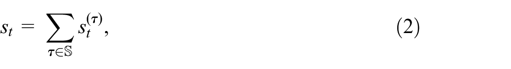
where
Remark 1. The seasonal periodicities in Equation (2) are given by the long-term average numbers of observations per reference period of interest, such as a week, month, year, etc. Accordingly, some of them are fractional due to the existence of leap years and the varying lengths of months in the Gregorian calendar, which will be considered throughout this paper. More precisely, the
Remark 2. The time-domain complexity of the seasonal component Equation (2) translates into a dense set of seasonal frequencies in the frequency domain. To see this, note that this set is given by
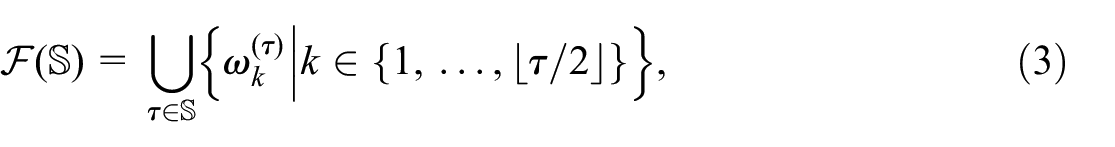
where
Remark 3. Regularization provides an alternative strategy for handling data with fractional seasonal periodicities. Instead of incorporating fractional periodicities directly into a model for the original data, regularization intends to construct modified data with a constant integer number of (partly artificial) observations per reference period. For example, when setting up a structural time series model for daily Dutch tax revenues, Koopman and Ooms (2003, 2006) transform the time axis and introduce artificial mid-month missing values so that each month consists of twenty-three banking days; those artificial missing values are then imputed straightforwardly during model estimation with the Kalman filter and smoother. In a similar way, Ollech (2021) uses cubic spline interpolation when modeling daily currency in circulation: each month is temporarily treated as if it had thirty-one days; leap years are temporarily shortened by skipping the records made on February, 29 (the resulting gaps are then filled with interpolations during the final calculation of the seasonally adjusted data).
Squared gain (8) for
3. Data Pretreatment
3.1. Linear Regression Model
Data pretreatment, or linearization, seeks to solve two problems prior to the application of any seasonal adjustment method: permanent removal of the calendar variation in Equation (1) and temporary outlier correction. Both problems are typically tackled jointly through running a time series regression of the form

where
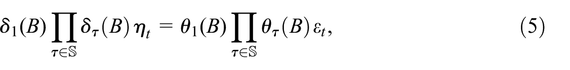
where

which is plugged into both the seasonal differencing and MA operators in Equation (5). For weekly data, for instance, we have

Note, however, that Equation (6) has no effect when
3.2. Model Properties
Approximation Equation (6) constitutes a fundamental principle of dealing with fractional periodicities. Therefore, it is interesting to study its effect on seasonal differencing from a theoretical standpoint. Moving to the frequency domain, the squared gain of

where

and

where
Remark 4. When
The principle in Equation (6) also facilitates the derivation of the pseudo-spectral density of the regression residuals
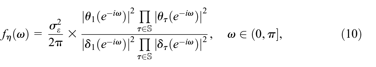
where the squared gains of the seasonal differencing operators are given by Equation (8) and those of the other involved operators read
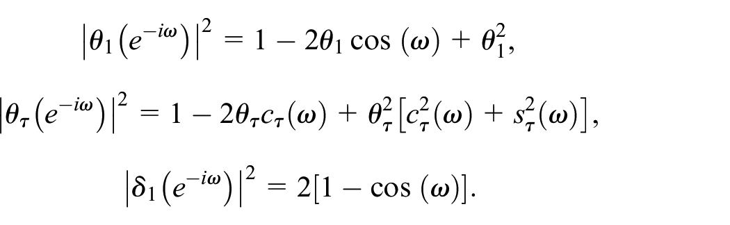
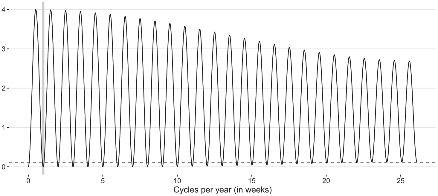
Figure 3 shows the pseudo-spectral density Equation (10) for the weekly EAM and four combinations of MA parameters. It is seen that, as for the classic Airline model, the non-seasonal MA parameter governs the shape of Equation (10) as
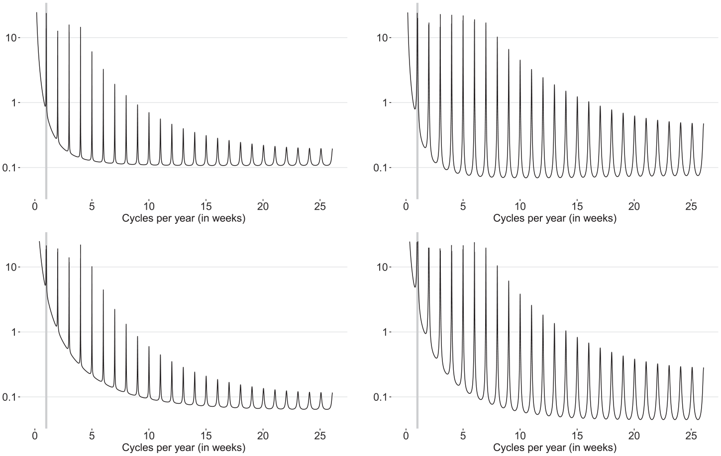
Pseudo-spectral density (10) with
3.3. Estimation and Forecasting
Estimation of pretreatment model Equations (4) and (5) is largely based upon the procedure described in Gómez and Maravall (1994). We briefly point out the basic principles; technical details can be found in Supplemental Appendix A.
When the observations are free of missing values, model Equations (4) and (5) is estimated by maximum likelihood (ML) with the differenced data. To this end, both the generalized least squares estimator of
Model estimation also includes an optional automatic search for additive outliers, level shifts and lag-
Given estimates
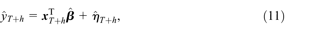
where

is the MSE-optimal

In practice,
3.4. Generalizations
A legitimate criticism of the EAM Equation (5) is the potential for excessive non-seasonal differencing introduced through the factorization Equation (9) even when the cardinality of
where
The principle in Equation (6) may provoke another EAM-related criticism as it sacrifices the seasonal unit root properties of
where
where
4. Extended ARIMA Model-Based Approach
Classic AMB seasonal adjustment for monthly and quarterly time series as implemented in the SEATS program is essentially organized in three steps; see, for example, Gómez and Maravall (2001b) and Maravall (1995) for extensive overviews and, in particular, the underlying modeling assumptions. In the first step, a seasonal ARIMA model is identified for the linearized observations. The default choice is the model found for the ARIMA errors by the TRAMO pretreatment routine but sometimes minor modifications, such as changes to the polynomial orders or variance inflation, need to be made. In a second step, the requested UC models are derived from the data model by means of the canonical decomposition (Hillmer and Tiao 1982), which basically postulates the uniqueness constraint that all (additive) WN extractable from the UC models is assigned to the WN irregular component, maximizing the latter’s variance amongst all admissible decompositions. To this end, the AR and differencing operators are first factorized through polynomial division and the radian frequencies of the roots obtained this way dictate their allocation to the UC models. Afterward, the pseudo autocovariance generating function (ACGF) of the data model is decomposed using a partial fraction expansion. In a third step, drawing on ideas of Burman (1980), Wiener-Kolmogorov (WK) filters are formed from the canonically decomposed model to finally calculate the minimum mean squared error (MMSE) estimates for the signals of interest; see Wiener (1949) for a general exposition of WK theory.
The extension of the classic AMB method follows the same key steps, using either the EAM Equation (5) or its generalization Equation (14) as a starting point. Thus, the unit roots at unity will be assigned to the trend-cycle while the non-stationary

and

where the orders of the MA polynomials
In some cases, the decomposition of the data model can be inadmissible in the sense that not all components have a non-negative spectrum for all frequencies. Hillmer and Tiao (1982) prove that an admissible decomposition exists if and only if the sum of the spectral minima of the components obtained through a unique partial fraction decomposition of the data model’s pseudo ACGF, where uniqueness is achieved by imposing specific constraints on the polynomial orders of the UC models, is non-negative. Inadmissibility can thus be seen to be equivalent to a negative variance of the WN irregular component in this unique decomposition. To solve this issue, the classic AMB approach implements several strategies including variance inflation, which is also used here. This strategy sets the variance of the WN irregular component in the aforementioned unique partial fraction decomposition to zero, essentially eliminating this component. As a result, the sum of the remaining trend-cyclical and seasonal components yields a new and decomposable data model from which the canonical decomposition and the requisite WK filters can be computed. Note that such a collapse of the WN irregular component may also happen in other strategies for overcoming inadmissibility; a prime example is the solution based upon the specification of top-heavy UC models (Fiorentini and Planas 2001).
Another modification to the classic AMB approach concerns MMSE estimation. WK filtering is predicated on the assumption of an invertible data model; however, the long MA polynomials that arise from large seasonal periodicities are typically prone to contain near-seasonal unit root factors that cause problems with respect to the convergence of the WK filters. Therefore, the extended AMB approach utilizes the state space representation of the canonically decomposed EAM and the Kalman filter and smoother (KFS), which avoids such non-invertibility issues and, in theory, yields the same results as the WK filter. The smoothing algorithm is implicitly selected by the user through the specification as to whether or not standard deviations of the components should be provided: if so, the diffuse square-root KFS is applied; otherwise, the fast disturbance smoother (Koopman 1993) with a diffuse initialization is used. Either way, the filtering recursions produce back- and forecasts for the UC estimates, which can then be aggregated to obtain alternative model-based back- and forecasts for the observed time series.
Signal extraction with the extended AMB approach can be performed either simultaneously or sequentially. A simultaneous extraction produces MMSE estimates for each UC in a single run; in this case, the application of the more robust square-root KFS is recommended, especially when
5. Extended X-11 Approach
The classic X-11 seasonal adjustment method derived in Shiskin et al. (1967) and reviewed in great detail in Ladiray and Quenneville (2001) is based upon an iterative application of predefined linear filters, which produces a sequence of preliminary, refined and final estimates for the trend-cyclical, seasonal and irregular components in Equation (1). During each of the X-11 iterations (labeled B through D), the following key four-step principle is applied twice. First, the trend-cycle is extracted from the input series through the application of a
The extended X-11 approach essentially adopts this iterative filtering process but incorporates some generalizations and modifications tailored to the peculiarities of infra-monthly data. The current implementation facilitates a sequential extraction of the seasonal patterns in Equation (2) without an automatic selection of trend-cycle and seasonal filters based on the
5.1. Trend-Cycle Filters
5.1.1. Preliminary Trend-Cycle Estimation
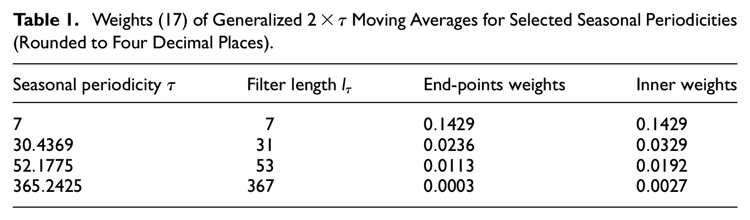
Preliminary trend-cycle extraction in the classic X-11 method is carried out with centered symmetric
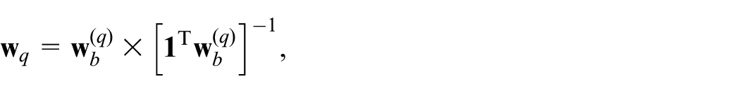
where
Weights (17) of Generalized
5.1.2. Refined and Final Trend-Cycle Estimation
The refined and final trend-cycle extraction filters of the classic X-11 method are essentially a set of prespecified weights for symmetric
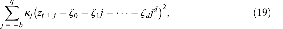
Trend-cycle estimation according to Proietti and Luati (2008) is founded on applying local polynomial regressions to the input series. Let

where
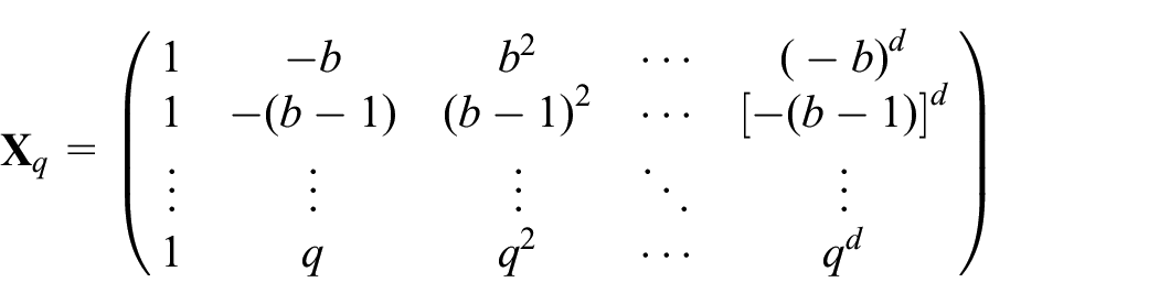
is the time-constant design matrix,
where
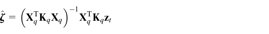
with
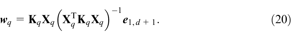
Assuming
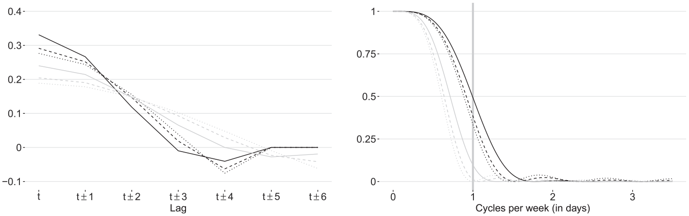
Coefficient curves (left panel) and squared gains (right panel) of symmetric kernel-based Henderson (solid lines), Epanechnikov (dashed lines), and unit-variance Gaussian (dotted lines) trend-cycle extraction filters (20) with
The weights of the corresponding asymmetric variants can be obtained for any choice of
where
5.2. Seasonal Filters
The classic X-11 method implements a set of predefined symmetric and asymmetric
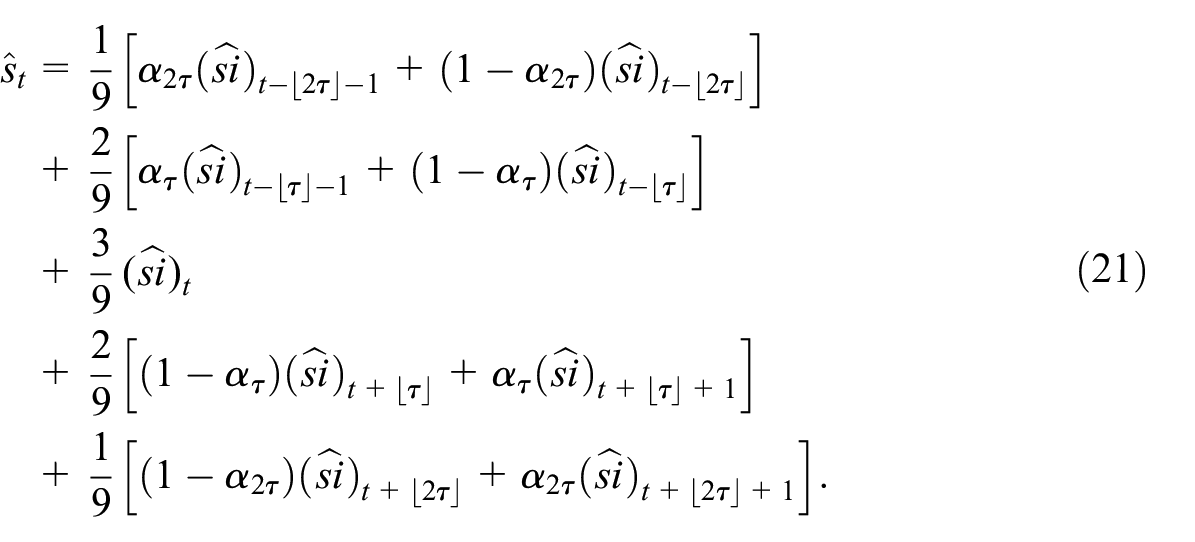
Figure 5 shows the squared gain of the (effective) seasonal extraction filter Equation (21) for
the squared gain of which is shown in Figure 6 for
Remark 5. Seasonal filters that incorporate principle Equation (6) operate at the exact non-integer seasonal periodicities but inevitably need to compromise some extraction power at the higher seasonal harmonics. Other seasonal adjustment approaches for infra-monthly time series possess a high extraction power at all seasonal harmonics at the expense of operating at slightly inaccurate integer periodicities, which is often achieved through temporary data regularization (see Remark 3). For example, the STL-based approach for daily data implemented in the
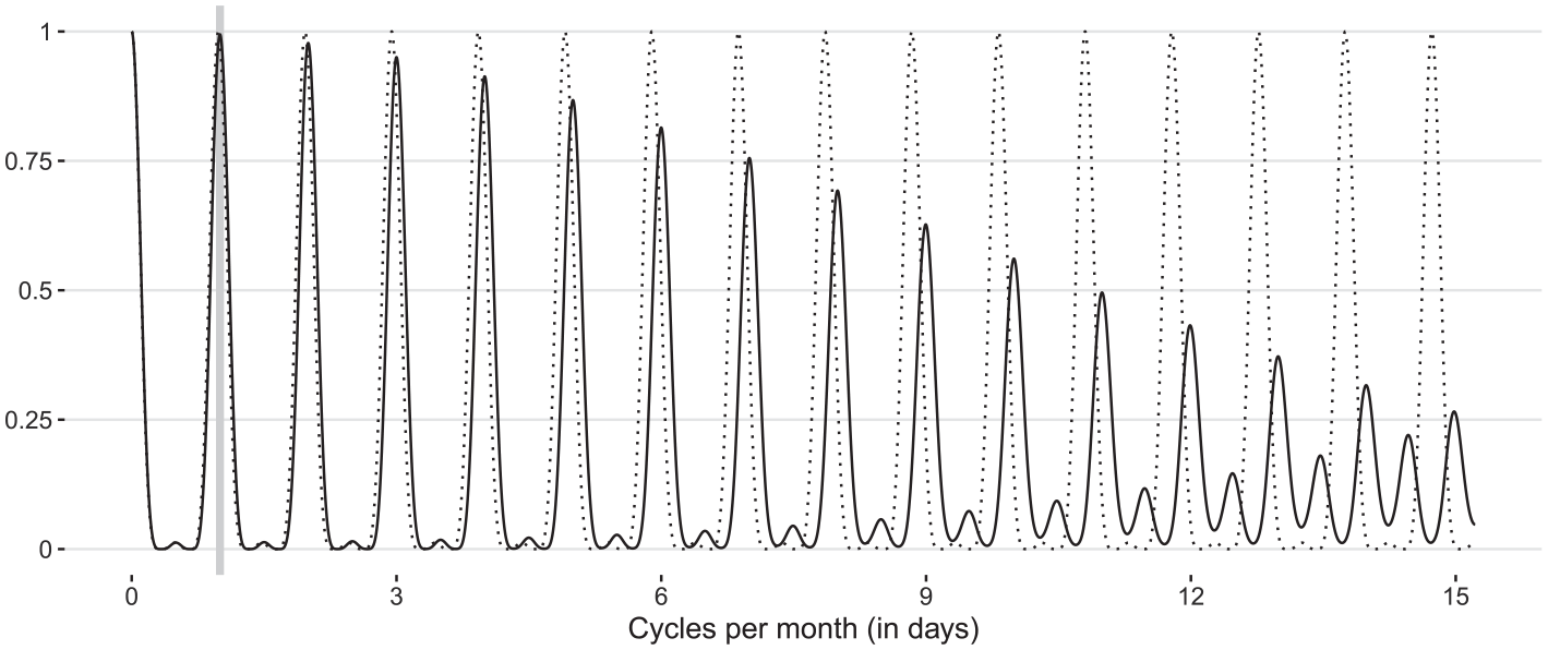
Squared gains of the symmetric
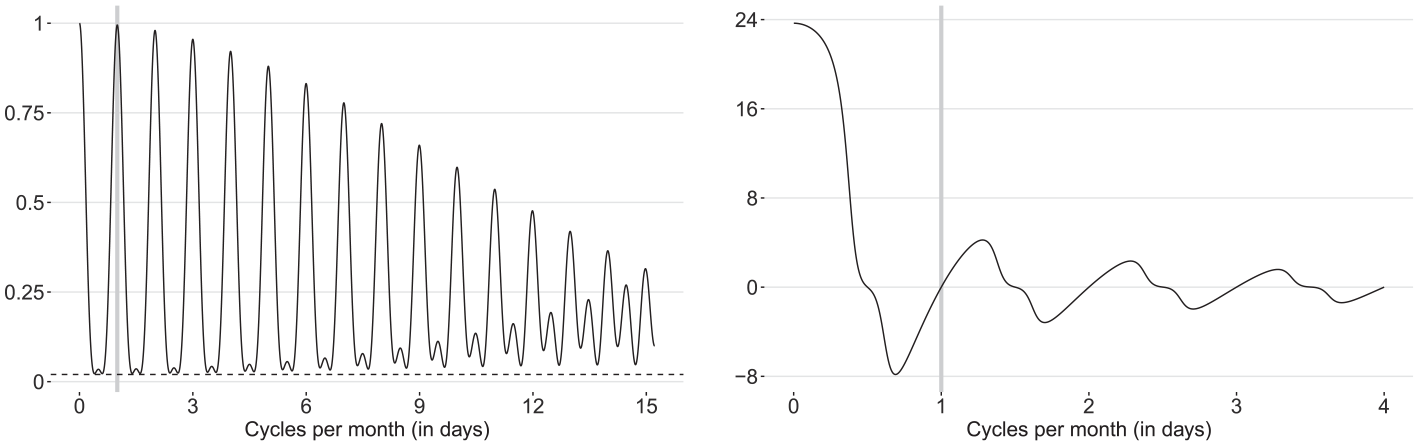
Squared gain (left panel) and phase shift in days (right panel) of the concurrent
6. STL Approach
The classic STL method developed in R. B. Cleveland et al. (1990) has been conceptualized originally as an alternative to X-11 and, therefore, also rests on the iterative application of linear filters. The filtering operations are organized in the so-called inner and outer loops; broadly speaking, each run through the inner loop produces updated estimates of the trend-cyclical and seasonal components and of the seasonally adjusted data whereas each pass of the outer loop generates an estimate of the irregular component as well as robustness weights.
The inner loop is essentially modeled on X-11’s basic four-step filtering principle outlined at the beginning of Section 5 to obtain the aforementioned refined estimates. However, STL’s fundamental modification is the replacement of X-11’s predefined trend-cycle and seasonal moving averages with linear extraction filters whose weights are derived through locally weighted scatterplot smoothing (LOESS), which is a specific form of a non-parametric univariate regression. The general LOESS objective function is similar to Equation (19) with
The optional outer loop yields an estimate of the irregular component, calculated as a residual by removing from the observed time series the trend-cycle and seasonal estimates obtained in the preceding inner loop. It also provides robustness weights based on the biweight kernel for the irregular component, which is conceptually akin to X-11’s extreme-value detection. During the next run through the inner loop, the combined neighborhood and robustness weights are then used in the LOESS regressions, that is, the principle of iterated WLS estimation is applied in Equation (19).
The current JD+ implementation is mostly in line with the practical recommendations given in R. B. Cleveland et al. (1990) that target “near certainty of convergence” of the STL trend-cycle and seasonal estimates. By default, two runs through the inner loop are carried out when no robustness weights are needed whereas fifteen runs through the outer loop, each time with a single run through the inner loop, are carried out otherwise. The polynomials in the LOESS objective function have orders
where
7. Structural Time Series Models
The pretreatment and seasonal adjustment methods discussed in Sections 3 to 6 perform data linearization and signal extraction in two separate steps. Structural time series (STS) models enable simultaneous estimation of all UCs in Equations (1) and (2); however, as opposed to the other methods, they require an a priori specification of the corresponding UC models, the aggregate of which then naturally constitutes the model for the observations (see Harvey 1989 as a standard reference).
In JD+, the most general trend-cycle specification within the STS framework is the local linear model given by


where
The seasonal component in (1) is specified through the West-Harrison representation (West and Harrison 1997). Assuming

where

where
with
where
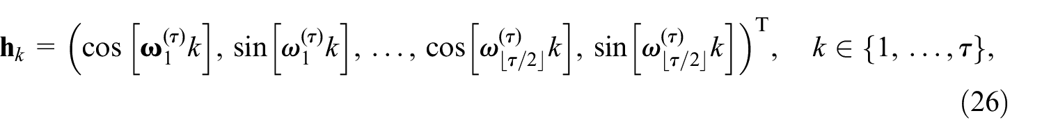
for the trigonometric seasonal model, noting that the last sine term in Equation (26) is dropped when
The entire STS model is put into a univariate linear Gaussian state space form, which also enables the inclusion of the calendar variation from Equation (1) by adding the requisite exogenous regression variables from (4) to the system matrix of the observation equation and the associated effects contained in
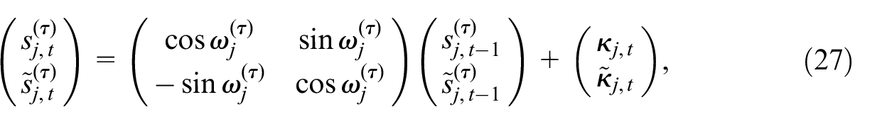
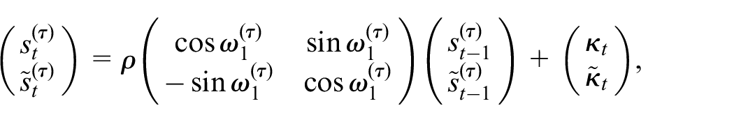
Remark 6. The above West-Harrison representation of the seasonal dynamics in Equation (1) might come across as somewhat unintuitive and opaque. Following the suggestion of an anonymous referee, we note that a simpler and more intuitive specification for each seasonal pattern in Equation (2) is given by
and
8. Applications
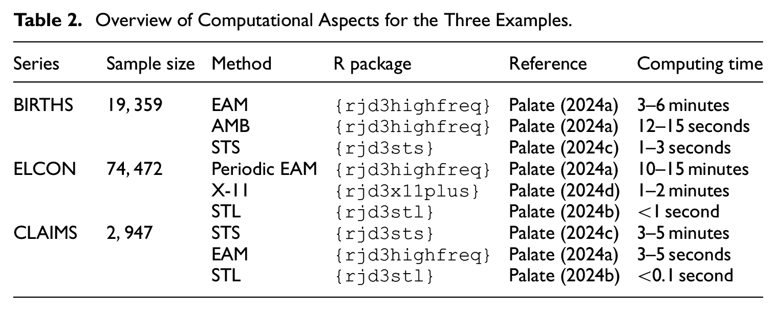
We consider three real-world examples to illustrate selected capabilities of the various JD+ methods discussed in Sections 3 to 7. Daily counts of births in France (BIRTHS) are used to compare data pretreatment and model-based signal extraction with the extended AMB and STS approaches for a multiplicative UC decomposition. Hourly realized electricity consumption in Germany (ELCON) is considered to illustrate periodic data pretreatment and to compare non-parametric signal extraction with the extended X-11 and STL methods. Finally, weekly initial claims for unemployment insurance in the United States (CLAIMS) are used for exploring differences between the STS and STL estimates for an additive UC decomposition, focusing on the COVID-19 pandemic phase. Throughout this section, data linearization will be based on the EAM generalization Equation (14) with
Overview of Computational Aspects for the Three Examples.
8.1. Daily Births in France
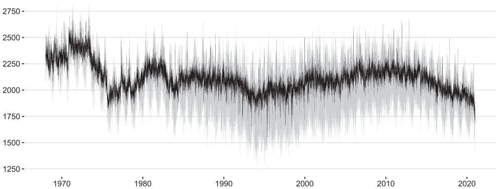
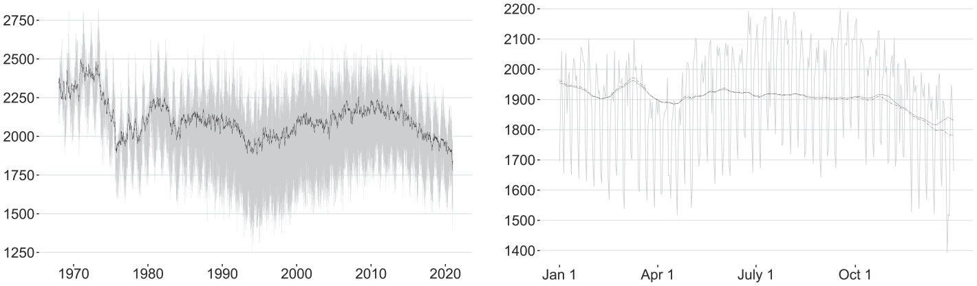
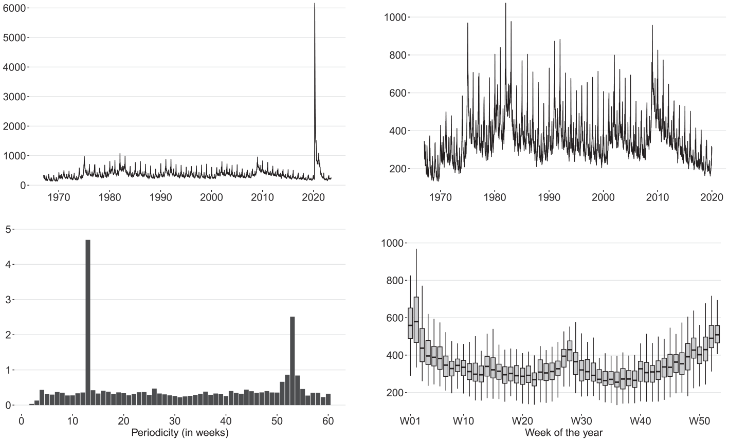
Figure 7 displays the daily BIRTHS series, covering the sample period of January 1, 1968 through December 31, 2020 (two top panels). The seasonal profile of the data is assessed through a sequence of point-wise generalized Canova-Hansen (CH) test statistics (Busetti and Harvey 2003; Canova and Hansen 1995) for the null hypothesis of no seasonality against the alternative of either deterministic or non-stationary stochastic trigonometric seasonality (row-
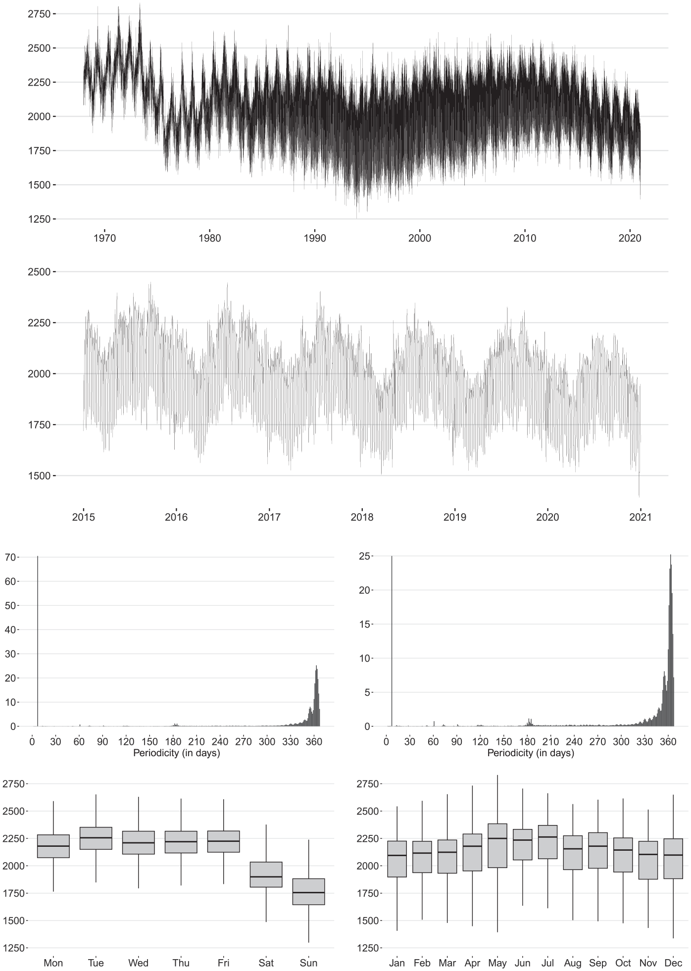
Seasonal profile of the BIRTHS series: raw data over the full span (top panel) and 2015 to 2020 span (row 2), point-wise Canova-Hansen test statistics for
8.1.1. Data Pretreatment and AMB Signal Extraction
We assume a multiplicative UC decomposition in Equation (1) and utilize pretreatment model Equations (4) and (5) to correct the BIRTHS series for the effects of the eleven public holidays in France, including automatic detection of additive outliers and lag-
Estimated Calendar Effects for the BIRTHS Series.
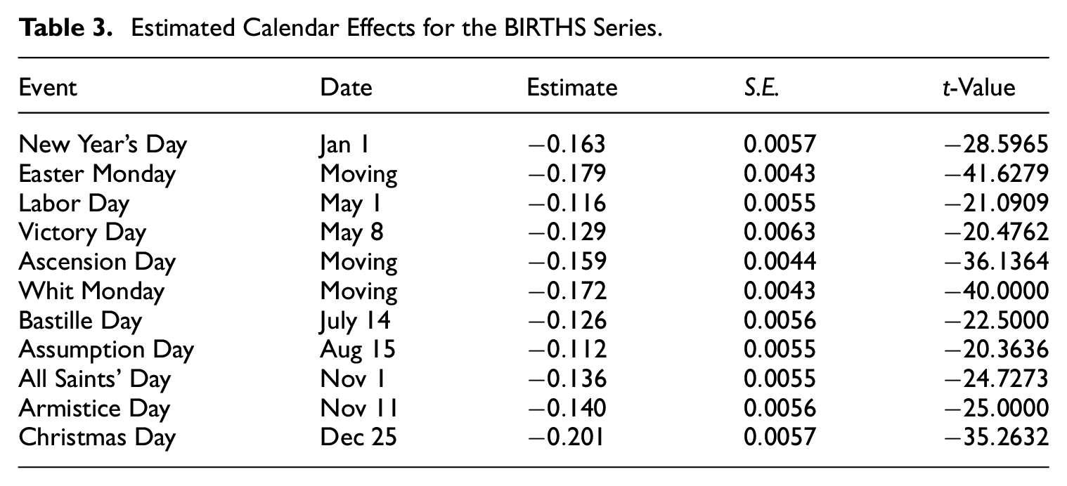
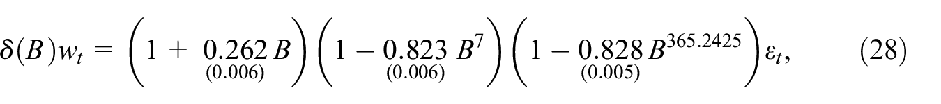
where
Model Equation (28) also lays the foundation for the sequential extraction of the DOW and DOY patterns with the extended AMB approach. To minimize risks associated with confounding, the DOW pattern is extracted first from the linearized logged BIRTHS series. Afterward, the DOY pattern is extracted from the DOW-adjusted linearized logged BIRTHS series. The estimated DOW pattern has a distinct time-varying amplitude that is largest during the mid-1990s whereas the estimated DOY pattern has a relatively constant amplitude but apparently undergoes some gradual structural infra-yearly changes after 1990 (see Figure 10 below). Both could be a consequence of the attempt to capture the changing volatility in the BIRTHS series during the 1980 to 2010 period. This possible explanation is supported by the fact that the volatility of the seasonally adjusted BIRTHS series remains relatively constant throughout the entire data span (Figure 8).
Raw (gray line) and seasonally adjusted BIRTHS series obtained with the extended AMB approach (black line).
Remark 7. An Associate Editor suggested to elaborate on the potential excessive non-seasonal differencing that may result in the EAM version Equation (5) and on its empirical relevance for seasonal adjustment. To this end, we compare the AMB trend-cycle estimates obtained from using
Raw BIRTHS series (gray line) and AMB trend-cycle estimates obtained with
8.1.2. Comparison with STS Approach
The classic Airline model for monthly and quarterly data is well-known to provide a good approximation to the reduced form of the so-called basic structural model (BSM) under certain parameter constraints (see, e.g., Maravall 1985). We are interested in finding out whether this property carries on to the EAM and specify the following additive BSM for the linearized logged BIRTHS series: the trend-cyclical component follows the local linear trend Equations (23) and (24); the DOW and DOY patterns are modeled according to the West-Harrison representation Equation (25) with trigonometric terms; finally, the irregular component in Equation (1) is assumed to be Gaussian WN with finite variance
where
The estimated UC innovation variances for this modified BSM are given by
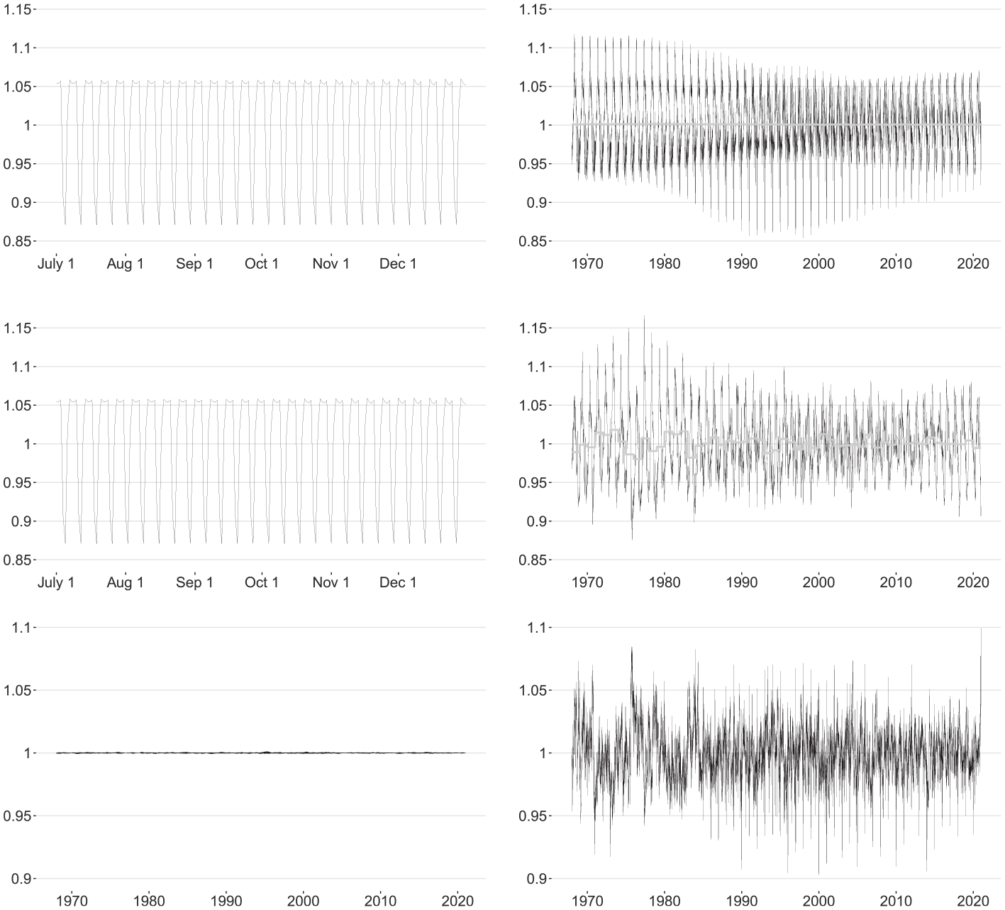
AMB (top panels) and STS (middle panels) signal estimates for the BIRTHS series, and their ratios (bottom panels): day-of-the-week pattern from July through December 2020 (left panels) and day-of-the-year pattern (right panels) including annual averages (gray line).
8.2. Hourly Realized Electricity Consumption in Germany
The hourly ELCON series is considered in units of gigawatt hours (GWh) for the period of January 1, 2015 (00:00 AM) through June 30, 2023 (11:00 PM). It covers electricity supplied to the network for the general supply, excluding electricity supplied to the railroad network and to internal industrial and closed distribution networks as well as electricity consumed by the producers. Since daylight saving time (DST) is in effect in Germany, the series is irregularly spaced, albeit slightly: twenty-four observations are available for each non-DST day; twenty-three observations are available for each DST starting day, that is, the last Sunday in March when the 02:00 AM record is skipped; twenty-five observations are available for each DST ending day, that is, the last Sunday in October when the 02:00 AM value is recorded twice. To regularize the ELCON series, we interpolate the missing 02:00 AM value for each DST starting day by the average of the adjacent 01:00 and 03:00 AM records and average the two 02:00 AM values for each DST ending day.
Figure 11 shows the seasonal profile of the regularized ELCON series. Electricity consumption tends to be higher in winter than in summer, leading to a
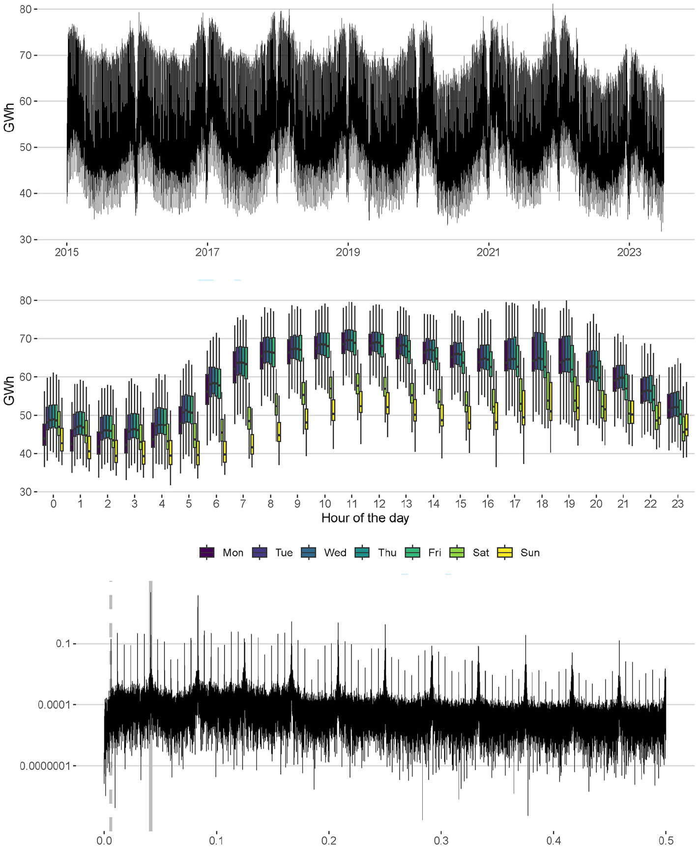
Seasonal profile of the ELCON series: raw data (top panel), boxplots grouped by the hour of the day and the day of the week (middle panel) and periodogram of the differenced logged data (bottom panel). Gray vertical lines (bottom panel) mark the chief hour-of-the-day (solid line) and hour-of-the-week (dashed line) frequencies.
8.2.1. Periodic Data Pretreatment
Preliminary empirical studies not discussed here failed to provide sufficient evidence in favor of the assumption of constant hourly calendar effects within each day in the logged regularized ELCON series. To allow for varying hourly calendar effects, we could use an appropriate set of hourly dummy regression variables in Equation (4) and set
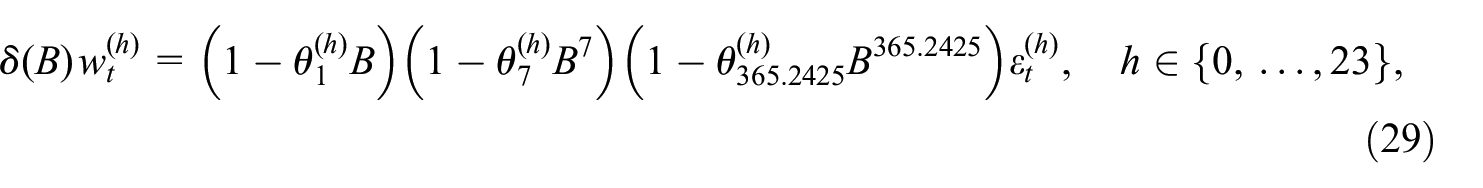
where

Note that in Equations (29) and (30) infra-daily seasonality is implicitly accounted for by the varying seasonal parameters across the twenty-four daily sub-models. Figure 12 plots the estimates of four calendar effects contained in

and finally transformed back to the original ELCON scale to form the precleaned hourly ELCON series.
Selected estimated calendar effects and MA parameters from periodic pretreatment model Equations (29) and (30): Easter Monday (top left panel), Labor Day (top right panel), Christmas Day (middle left panel), New Year’s Eve (middle right panel),
8.2.2. Non-Parametric Signal Extraction
Based on visual evidence (Figure 11), we now set

X-11 (black line) and STL (gray line) signal estimates for the ELCON series: hour-of-the-day pattern over June 24 to 30, 2023 (top left panel), hour-of-the-week pattern from May through June 2023 (top right panel), hour-of-the-year pattern (bottom left panel), and ratio of the combined adjustment factors (bottom right panel).

Raw (light gray line) and seasonally adjusted ELCON series obtained through the extended X-11 (black line) and STL (gray line) approaches over the full span (top panel) and 2022 to 2023 span (bottom panel).
8.3. Weekly Initial Claims for Unemployment Insurance in the United States
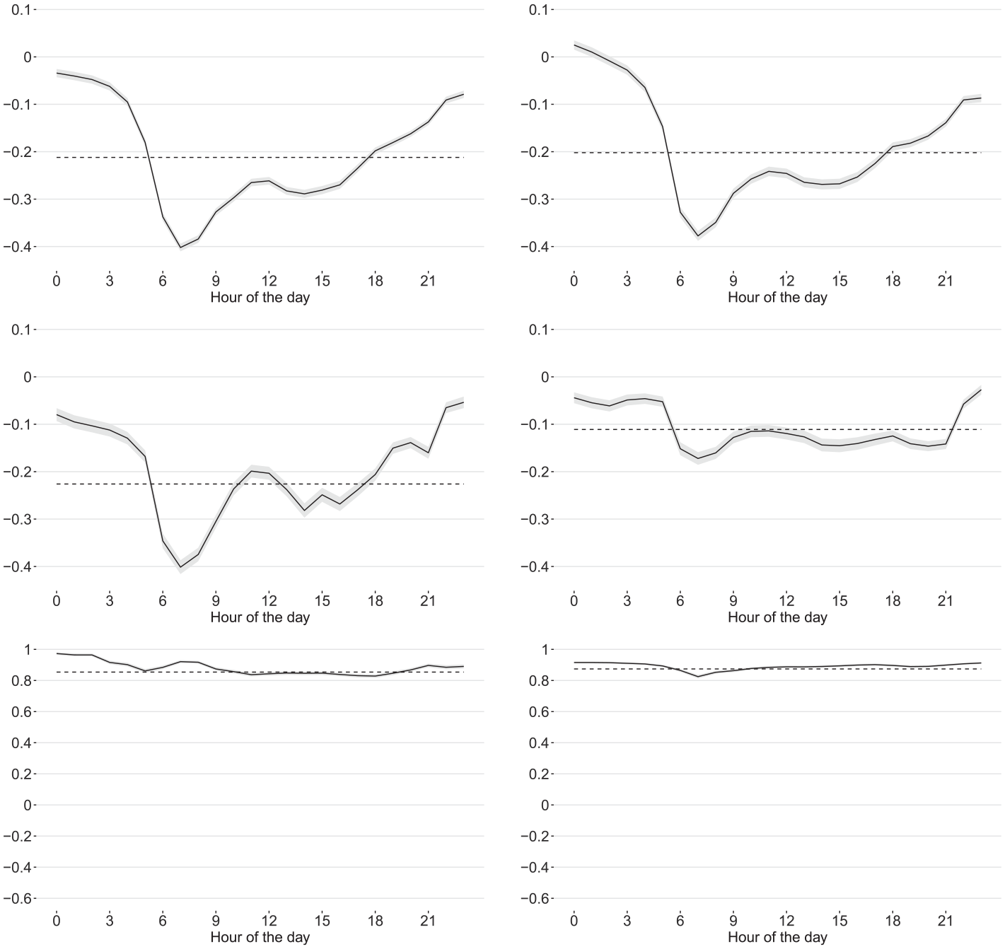
The weekly CLAIMS series is considered as of 1967 W01 up to 2023 W25, with economic activity being measured from Sunday through Saturday. Shorter versions of this series have also been analyzed in earlier studies on weekly data (e.g., Abeln and Jacobs 2022; Cleveland et al. 2018; Cleveland and Scott 2007; Evans et al. 2021; Proietti and Pedregal 2023).
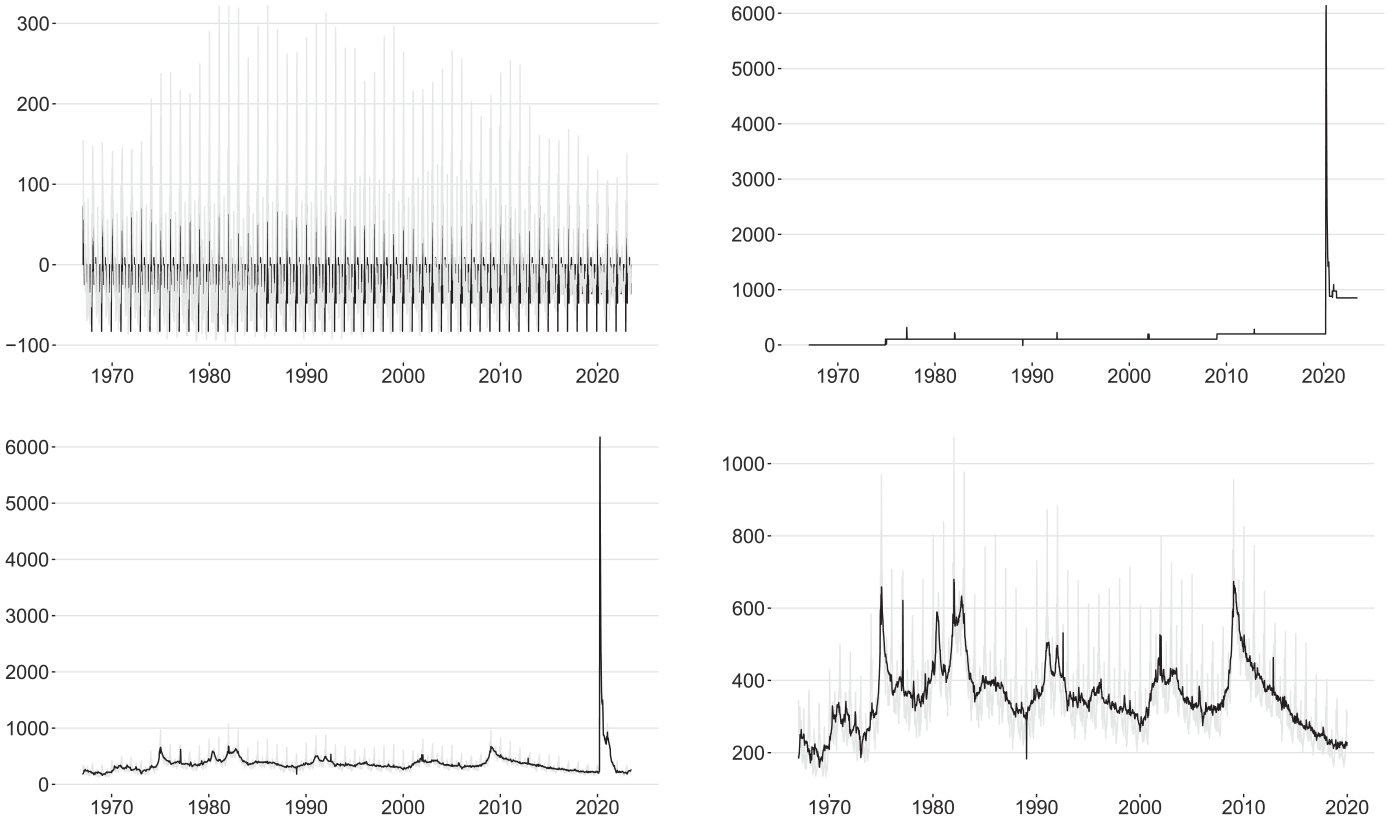
The seasonal profile of the CLAIMS series is shown in Figure 15. The claims meander roughly between
Seasonal profile of the CLAIMS series (thousands): raw data over the full span (top left panel) and pre-pandemic span (top right panel), point-wise Canova-Hansen test statistics for
8.3.1. Basic Structural Model
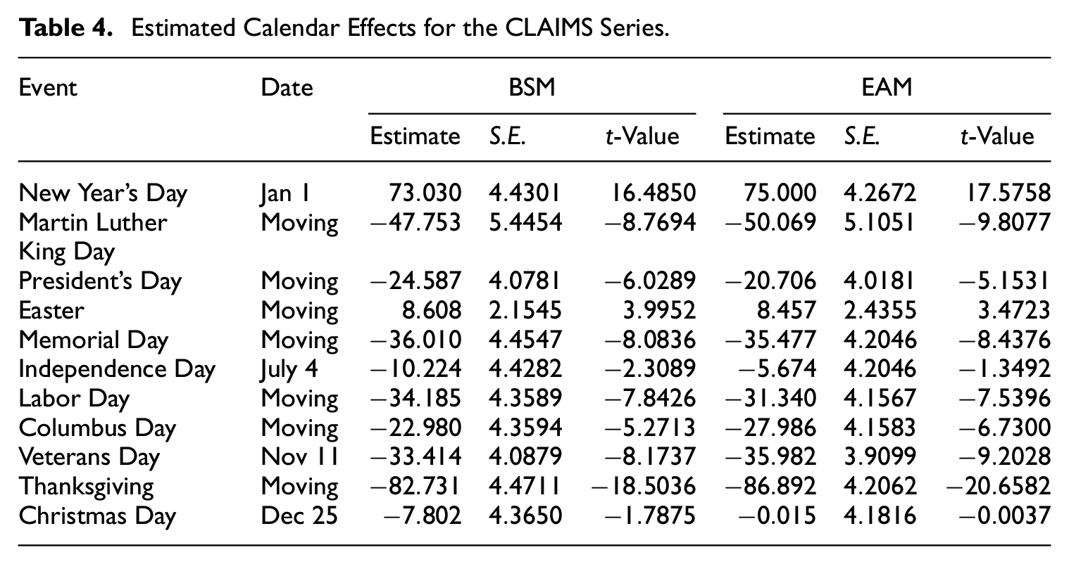
We specify an additive BSM for the untransformed CLAIMS series, noting that this choice of UC decomposition is in line with official seasonal adjustment practices at the U.S. Bureau of Labor Statistics (BLS) in the wake of the COVID-19 pandemic outbreak (in fact, the decomposition scheme has been changed temporarily from multiplicative to additive between March 2020 and June 2021). The trend-cycle is modeled as a local linear trend according to Equations (23) and (24), the WOY pattern follows the trigonometric seasonal model Equation (26) using the full set of twenty-six harmonics, and dynamics associated with federal holidays are captured by a set of eleven weekly dummy regression variables (with the effect of New Year’s Day being assigned to W02 as in W. P. Cleveland et al. 2018). Besides an automatic search for additive outliers and level shifts with series-length-adjusted
Estimated Calendar Effects for the CLAIMS Series.
Smoothed estimates for various unobserved components in the CLAIMS series (thousands): calendar component (black line) and trigonometric WOY pattern (gray line; top left panel), outlier component (top right panel), raw (gray line) and seasonally adjusted (black line) data over the full span (bottom left panel) and pre-pandemic span (bottom right panel).
Remark 8. The main purpose of the CLAIMS example is to illustrate the STS modeling framework currently implemented in JD+. It should be noted, however, that our underlying acceptance of a time series model with constant (regression) parameters may be questioned for such a long data sequence. As pointed out by an anonymous referee, the data generating process of the CLAIMS series has undergone several changes over time. For example, every U.S. federal state has different laws on eligibility for unemployment insurance claims; these laws have changed a lot. In addition, claims needed to be filed in local offices in the distant past whereas online submissions are the norm nowadays. Hence, some holiday effects may have become less significant, or even insignificant, in recent years. Despite these valid concerns, we believe that the above BSM specification is good enough for serving our primary goal here; however, we agree that a more nuanced modeling of the CLAIMS series is advisable when targeting other purposes, such as providing guidance for policy makers. In such a case, separate treatments of shorter non-overlapping data segments, constant-parameter models with additional holiday regression variables for exceptionally early or late occurrences of some moving holidays in some years and day-of-the-week interactions of some fixed holidays, or time series models with time-varying parameters could be considered. Using temporary changes, or other types of transitional outliers, in place of the two level shift sequences could especially improve the modeling of the COVID-19 pandemic phase; in fact, the BLS has implemented such replacements during recent regular revisions of its seasonal adjustment specifications (see U.S. Bureau of Labor Statistics 2024 for more details).
8.3.2. COVID-19 Modeling and Comparison with STL Approach
Another anonymous referee pointed out that according to Abeln and Jacobs (2022) the robust STL method does not require the two level shift sequences, or other forms of outlier modeling, for taking the COVID-19 pandemic phase into account. To check this claim, we compare the smoothed BSM estimates of the seasonally adjusted CLAIMS series to their (additive) non-robust and robust STL counterparts. Utilizing bandwidths over fifty-five and eleven observations for the trend-cycle and seasonal LOESS smoothers, respectively, both STL estimates are calculated from the holiday-corrected CLAIMS series that is still contaminated with all outliers present in the raw data. Note, however, that pretreatment model Equations (4) and (5) is fed not only with the eleven user-defined holiday variables but also with the two level shift sequences and the same parameter choices for automatic outlier detection that have been specified for the BSM approach. This is done to avoid distortions to the estimated holiday effects, which are likely to arise from a willful ignorance of other known exogenous effects, or any other model misspecification. The estimated EAM-based holiday effects are in general very similar to the BSM estimates, with the more obvious insignificance of the Independence Day and Christmas Day effects being the most notable differences (see columns 6–8 of Table 4).
Mirroring Abeln and Jacobs (2022, Fig. 3), Figure 17 shows that the seasonally adjusted CLAIMS series obtained from the BSM and robust STL approaches are visually almost indistinguishable during the COVID-19 pandemic phase (top panel). The only exception are some minor deviations around the 2020/2021 turn of the year, which may be traced back to the fact that in model (4) and (5) three outliers have been automatically detected between 2020 W50 and 2021 W08 that were not identified by the BSM routine (both automatic detection routines find virtually the same outliers in the pre-pandemic span). Emphasizing the importance of applying STL with robustness weights when no outlier pretreatment is conducted, Figure 17 also highlights severe biases in the seasonally adjusted CLAIMS series obtained from the non-robust STL approach (bottom panel). Not only does the level of this seasonally adjusted series exhibit short-lived downward distortions by up to half a million cases in the March and April figures (which even become negative in 2019), it displays very long periods of visible upward biases in the other months as well. These weird and clearly undesired effects extend beyond the 2019 to 2021 span shown in Figure 17 but eventually fade out. Overall, our findings support the above claim made by Abeln and Jacobs (2022) with respect to the robust STL method, although it is not obvious to us how these authors have dealt with the calendar variation in the CLAIMS series.
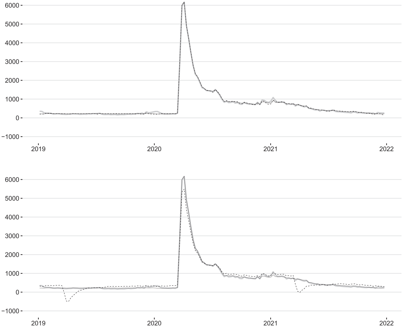
Raw (gray line) and seasonally adjusted CLAIMS series (thousands) obtained from the STS (solid black line) and STL (dashed black line) approaches applied to the EAM-based holiday-corrected data: robust (top panel) versus non-robust (bottom panel) STL approach.
9. Summary
We gave an elaborate description of the modeling and signal extraction methods for infra-monthly time series implemented in JDemetra+ 3.0. In particular, we highlighted the key modifications that needed to be made to official statistics’ established pretreatment and seasonal adjustment approaches in order to take the peculiarities of such granular data into account. Pretreatment for outliers and calendar variation is handled through a time series regression in which the disturbances are assumed to follow an extension of the classic Airline model, which enables the incorporation of multiple seasonal patterns and fractional seasonal periodicities. Using a first-order Taylor expansion, fractional powers of the backshift operator are approximated by a weighted average of the two adjacent integer-valued powers of the backshift operator. The same Airline-type model provides the foundation for an extended ARIMA model-based seasonal adjustment approach based on the classic concept of a canonical model decomposition. MSE-optimal estimates for the requisite unobserved components are then obtained through the Kalman filter and smoother applied to the state space representation of the decomposed extended Airline model. The above Taylor approximation is also adopted in an extended X-11 seasonal adjustment approach to retain applicability of the classic
The methodological toolbox of JDemetra+ 3.0 is already quite rich but still leaves room for enhancements. First of all, some classic concepts that have proven to be useful for the seasonal adjustment of monthly and quarterly data should be made (more easily) accessible for the treatment of infra-monthly data as well. Prime examples are bias corrections for non-linear data transformations and the use of forecast extensions within non-parametric seasonal adjustment methods to enable the application of less asymmetric, or even symmetric, linear extraction filters near the end-points (which is likely to reduce real-time revisions in signal estimates). The addition of temporary changes and/or otherwise smooth transitional outliers, log/level and seasonality tests as well as tailored diagnostics (e.g., McElroy 2021) would definitely help to automate the entire pretreatment process for infra-monthly data. Several alternatives, such as models Equations (15) and (16) with either the full or a reduced set of seasonal harmonics as well as (structural) models with time-varying regression parameters, provide room for further improvements.
Apart from that, future research could also pay attention to adequate data-driven selections of trend-cycle and seasonal extraction filters for non-parametric seasonal adjustment methods. For example, the framework of Proietti and Luati (2008), which is already utilized in the extended X-11 approach, enables the identification of the optimal bandwidth for trend-cycle extraction through cross-validation given a prespecified polynomial degree and set of kernel weights. As regards model-based signal extraction, saturated seasonal models, such as the West-Harrison representation Equation (25), could be over-parametrized and computationally infeasible for large seasonal periodicities (see the BIRTHS example discussed in Section 8.1). Therefore, structural time series models with an alternative representation of seasonality, such as the more intuitive trigonometric specification (27), and/or with seasonal interactions embedded in a correlated unobserved components framework (cf. Hindrayanto et al. 2019; Koopman and Lee 2009) could be more useful in practice and may be added in a future version of JDemetra+. Periodic cubic splines (Harvey and Koopman 1993; Harvey et al. 1997) seem to be another promising alternative; however, a strategy for automatically picking both the number and positions of the constituting knots still needs to be worked out. Some inspiration might be drawn from the LOESS-based approach discussed in Proietti and Pedregal (2023).
Besides methodological improvements, it would also be interesting to compare the signal extraction methods currently implemented in JDemetra+ 3.0 with other methods. Using daily and weekly economic time series, we are currently evaluating the real-time revisions in concurrent seasonal adjustments carried out with the extended ARIMA model-based and X-11 approaches and with the STL-based approach available in the
Supplemental Material
sj-pdf-1-jof-10.1177_0282423X241277602 – Supplemental material for Seasonal Adjustment of Infra-Monthly Time Series with JDemetra+
Supplemental material, sj-pdf-1-jof-10.1177_0282423X241277602 for Seasonal Adjustment of Infra-Monthly Time Series with JDemetra+ by Karsten Webel and Anna Smyk in Journal of Official Statistics
Footnotes
Acknowledgements
We thank Jean Palate of the National Bank of Belgium for providing detailed answers to all our questions about the methods implemented in JD+. We also thank Christiane Hofer of the Deutsche Bundesbank, James Livsey of the U.S. Census Bureau and the participants of the 2nd Workshop on Time Series Methods for Official Statistics held at the OECD in Paris on September 22–23, 2022 for their valuable comments on an earlier version of the paper. Last but not least, we are very grateful to an Associate Editor and three anonymous referees for their helpful comments and suggestions that greatly improved our paper.
Authors’ Note
The views expressed on statistical issues are those of the authors and do not necessarily reflect the views or policies of the Deutsche Bundesbank, Insee, or the Eurosystem. All time series analyzed in this paper are freely available from public data sources.
Funding
The author(s) received no financial support for the research, authorship, and/or publication of this article.
Supplemental Material
Supplemental Material for this article is available online.
Received: September 2023
Accepted: July 2024
References
Supplementary Material
Please find the following supplemental material available below.
For Open Access articles published under a Creative Commons License, all supplemental material carries the same license as the article it is associated with.
For non-Open Access articles published, all supplemental material carries a non-exclusive license, and permission requests for re-use of supplemental material or any part of supplemental material shall be sent directly to the copyright owner as specified in the copyright notice associated with the article.