
Abstract
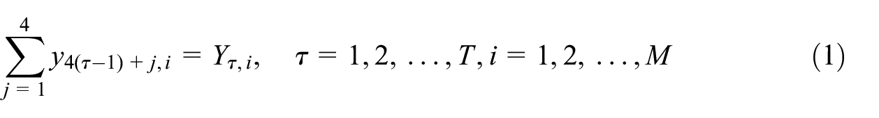
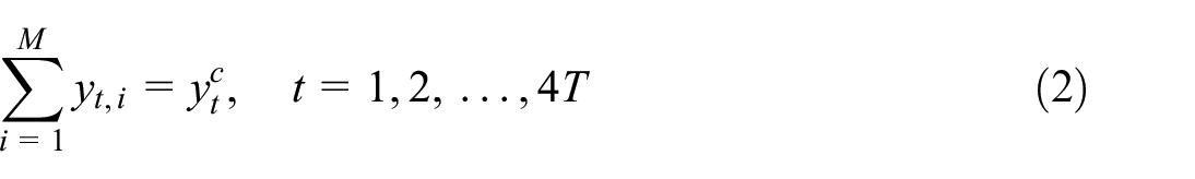
We propose a simple smoothing method for the spatiotemporal disaggregation of economic time series. Contrary to the existing methods, our approach does not require exogenous regressors and can therefore be used for countries lacking long and reliable series of regional economic indicators. The proposed method can also be applied sequentially, implying that one needs to revise only the estimates for the last low-frequency period when new data are disaggregated. This is a convenient feature when historical estimates are of interest. We apply this method to disaggregate annual real GDP data for Polish regions into quarterly series and compare the results with the series obtained from a multivariate linear regression-based procedure, considering the differences between the estimates and the consequences for regional recession dating. We also examine the nowcasting performance of the smoothing algorithm and find that it is superior to the regression-based alternative for most of the studied sample lengths and horizons up to a year.
1. Introduction
Conceptualizing efficient economic policies and conducting robust research requires reliable and up-to-date data. For economic activity, such data are available mainly at the national level. Flash estimates of quarterly gross domestic product (GDP) are usually released after several weeks, whereas various forecasts and nowcasts are published much earlier. The situation is much worse at the regional level. Typically, only annual GDP series are available, and publication delays can last one year or even longer. The USA and the UK are notable exceptions, as their statistical offices publish quarterly regional GDP series with delays of three and six months, respectively.
Several spatiotemporal disaggregation methods have been developed to address the missing regional data problems. All of these methods are statistical approaches that estimate the missing high-frequency series using a set of auxiliary regional indicators and standard temporal and spatial contemporaneous constraints. For example, Mazzi and Proietti (2017, 234) distinguish among three classes. First, observation-driven models extend the seminal regression-based model developed by Chow and Lin (1971; Cuevas et al. 2015; Di Fonzo 1990; Pipień and Roszkowska 2015; Proietti 2011; Rossi 1982). Second, parameter-driven methods aim to build a joint structural model for the estimated series and auxiliary indicators, usually using dynamic factor models (Moauro and Savio 2005; Proietti and Moauro 2006) or mixed-frequency Bayesian vector autoregressive models (Koop, McIntyre, and Mitchell 2020; Koop, McIntyre, Mitchell, and Poon 2020; Lehmann and Wikman 2022). Third, semiparametric approaches encompass Denton’s multivariate benchmarking method (Di Fonzo and Marini 2011) and the polynomial method proposed by Hedhili Zaier and Trabelsi (2007).
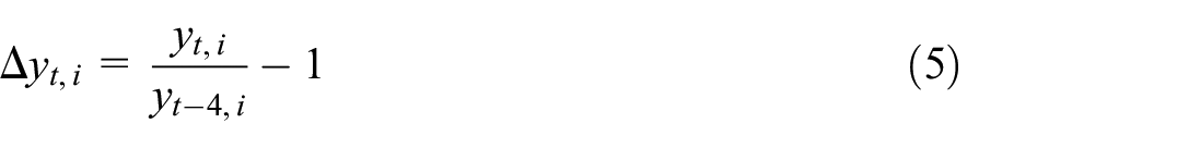
While accounting for additional information usually improves estimates, it also leads to some difficulties. First, it requires reliable indicators. For many countries, particularly the post-communist countries of Central and Eastern Europe, the high-frequency series related to economic activity at the regional level are usually short. Additionally, their quality is relatively low because of idiosyncratic shocks or breaks. For example, Statistics Poland—the national statistical agency—is one of the world leaders in data coverage and website availability according to the ODIN ranking (Open Data Watch 2021). However, at the NUTS-2 regional level in Poland, there are only five series related to cyclical economic activity measured at the quarterly frequency available for the 2006 to 2021 period. Of these, one is the unemployment rate, which, because of strong employment protection in Poland, lags the business cycle considerably (see Grabek and Kłos 2013, for the evidence for Poland and Di Iorio and Triacca 2022, for some other European countries) and therefore cannot be a reliable regressor for quarterly GDP estimation. The industrial production and investment series are also plagued with outliers, where the annual change exceeds 40% and even reaches more than 100%. And these numbers do not refer to the coronavirus disease (COVID-19) period.
The second problem is practical. As data for a new period are released, disaggregating them using statistical techniques usually requires revising all the previously disaggregated series. For nowcasting or forecasting purposes, this is just a minor side effect; however, when the historical series are of interest, the drawback becomes severe, even if it can be administered through the official data revision policy. Although the estimates from short time series are likely to be more sensitive to new observations, longer series are not immune to this problem either.
For example, the cyclical estimates of the quarterly gross value added (GVA) for Great Britain’s regions that are based on the half-century-long sample (Koop, McIntyre, Mitchell, and Poon 2020, the disaggregated series are available at https://www.escoe.ac.uk/regionalnowcasting/; accessed 8.09.2022) also vary considerably between editions. The mean absolute difference between the estimates of the real quarter-on-quarter GVA obtained in the last quarter of 2018 and the last available results from the second quarter of 2021 ranges between 0.3 and 0.7 p.p., representing 9.6% to 28.6% of the unconditional standard deviation of the series. Even the differences between the consecutive estimates are non-negligible. They are equal to 0.1 to 0.4 p.p., that is, 3.3% to 17.7% of the unconditional standard deviation for the first two quarters of 2021. To some extent, these differences may result from the input data revisions. However, they not only occur at the end of the sample, where the input series are revised, as their sizes are approximately the same as at the beginning of the investigation period.
Finally, as noted by Mazzi and Proietti (2017, 233), official statistical agencies still prefer univariate methods because they are simpler and less computationally intensive. The multivariate approaches can only be applied by agencies that employ highly trained staff with experience in disaggregation problems, such as in Italy or Spain.
Herein, we propose an alternative spatiotemporal decomposition method that uses a smoothing criterion. We postulate that the annual growth rates of the disaggregated series should be as smooth as possible. This idea extends to the first algorithms for univariate disaggregation proposed by Boot et al. (1967) that can be viewed as a special application of the adjustment problem considered by Denton (1971) and Cholette (1984). To our best knowledge, it has never been utilized for multivariate cases.
Unlike other methods, ours does not require auxiliary regressors and can be applied sequentially. This means that previous estimates need not be revised entirely when new data is disaggregated––only the last part needs to be updated. Additionally, our method is computationally simple because it requires solving a set of rather simple, constrained optimization problems, as shown in the next section. These advantages make the smoothing procedure a reasonable choice for countries that lack long and reliable series of regional statistics and when historical estimates are of particular interest.
Focusing on growth rates makes our procedure closely related to the growth-preserving benchmarking and reconciliation methods (Bozik and Otto 1988; Causey and Trager 1981; Dagum and Cholette 2006; Di Fonzo and Marini 2012, 2015; Titova et al. 2010; Trager 1982), particularly when looking at the optimization problems. However, contrary to these studies, we use annual growth rates instead of period-by-period ones.
We apply our method to disaggregate the annual real GDP series for 16 NUTS-2 regions of Poland. The annual data on regional GDP in Poland are published with substantial delays. Nominal values are released after one year, whereas the real series are published two years after the end of the year of interest. Like other post-communist countries of Central and Eastern Europe, Poland underwent a complete transformation of its socioeconomic life, including the administrative division of the country and the functioning of public statistics. Therefore, as discussed earlier, it also lacks long and reliable series of regional business cycle benchmarks.
We consider two versions of the smoothing algorithm. The baseline sequential approach divides the disaggregation problem into a set of annual sub-problems. In contrast, the one-step variant solves the problem in one step for the entire study period. The results show that the differences between the two procedures are minimal. We also compare the disaggregated series with the results of a multivariate linear regression-based procedure. We consider the differences between the estimated growth rates and the consequences for regional recession dating.
Finally, we also examine the nowcasting abilities of the smoothing approach by running a pseudo-real-time nowcasting experiment. By nowcasting, we mean estimating the quarterly regional values when the annual regional totals are unavailable. Theoretically, because the smoothing approach relies solely on the persistence of the disaggregated series and the current quarterly country-level data, it is expected to be inferior to the regression-based methods guided by auxiliary indicators. However, it is unclear to what extent the aforementioned problems of short samples and poor data quality affect the benchmarking procedures and decrease their nowcasting abilities.
The remainder of the article is organized as follows. Section 2 presents the procedure. Section 3 is devoted to the disaggregation results, whereas Section 4 presents the nowcasting experiment. Section 5 concludes the study.
2. The Procedure
2.1. The Preliminaries
This study uses the following notation: capital letters represent annual variables, whereas small letters denote quarterly data. The procedure takes two series as inputs: the annual data on regional GDP levels
The unknown quarterly regional data should satisfy the set of temporal and contemporaneous spatial constraints:
The first condition represents the aggregation of quarterly data to the observed annual series, and the second constraint implies that the regional data sum up to the observed country series. Constraints, Equation (1) and (2), imply that the input series should satisfy the following set of conditions:
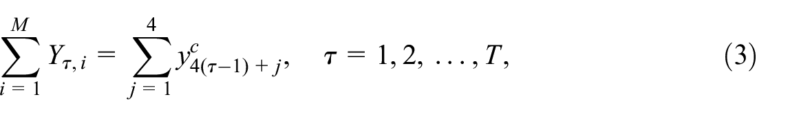
so that the sum of the annual regional values is equal to the sum of the quarterly country-level series for a given year. In practice, the condition in Equation (3) might not be satisfied because of rounding errors, mainly when the series are created from volume indices. In this case, an initial rebalancing procedure should be applied to establish the series’ consistency. The simplest one is to adjust the regional values proportionally to match the sum of the quarterly country-level values:
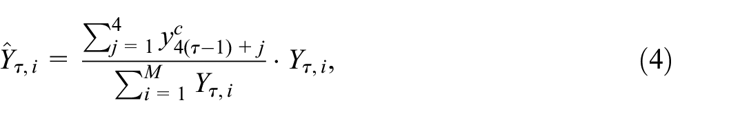
where
2.2. The Optimization Problem
In this study, we disaggregate the two input series so that the resulting year-on-year (y-o-y) growth rates of quarterly regional GDP are as smooth as possible and satisfy the constraints in Equation (1) and (2). More formally, let
The set of quarterly regional GDP series
where
T9he weighting scheme plays a vital role in the optimization problem because the contributions of different regions to GDP and, in turn, to contemporaneous constraints, Equation (2), differ considerably. Without the weights, the algorithm would prefer smoothing the growth rates in small regions over the most important ones.
Following Di Fonzo and Marini (2012, 2015; see also Brown 2010; Causey and Trager 1981), we use the interior point Newton-type algorithm to solve the smoothing problems. In the case of growth rate smoothing problems, it also delivers fast and accurate solutions.
2.3. The Sequential Solution to the Optimization Problem
Generally, the optimization problem Equation (6) should be solved in one step using a numerical solver. Such an approach, however, requires revising all the disaggregated series when data for a new period are added, leading to the frequent data revision problem discussed in Introduction. Fortunately, the revisions are tiny and an alternative, sequential approach to optimization can be applied. It fixes most of the already disaggregated series and adjusts only the most recent estimates to disaggregate the new data. Therefore, this version is no longer subject to substantial revisions of the earlier estimates. Notably, the solution obtained with the sequential disaggregation differs from that obtained with the one-step procedure. However, as documented in the next section, the differences are minimal.
The sequential procedure entails as follows: in the first step, the problem Equation (6) is solved for some initial
In the second step, we add the data for the next year
where
In this study, we treat the sequential procedure as the baseline algorithm.
2.4. Nowcasting
By nowcasting, we mean estimating the missing quarterly regional GDP series for periods when no annual regional values are available, but the quarterly country-level data are known. In this case, we solve the smoothing problem Equation (6) without the contemporaneous constraints Equation (1). Formally, let
where
2.5. The Multivariate Regression-Based Method
In the study, we compare the performance of the smoothing algorithm a multivariate regression-based method. This approach uses a set of auxiliary high-frequency, region-level regressors that serve as benchmarks for disaggregated series. We consider the following optimization problem:
where
To nowcast with the regression-based method, we use the estimated regression coefficients
where
We apply an iterative algorithm to solve the regression problem Equation (9). First, given the starting values of
3. The Disaggregation Results
In this section, we use the method described above to disaggregate the real GDP data for Poland. We use the results to analyze business cycles at the regional level and compare the results with the multivariate benchmarking/regression method.
3.1. The Data
Statistics Poland publishes the regions’ annual growth rates of chain-linked GDP volumes. The data are available for the 2004 to 2019 period. For 2020, only nominal GDP data are published. Therefore, we approximate the regional growth rates of GDP volumes for 2020 by deflating the nominal growth rates for that year by the regional price indices for the previous year (the price indices for 2020 are also unknown). Subsequently, we create the chain-linked volume GDP series using the growth rates described above and the GDP series at the current prices for 2003 published by Statistics Poland. We also use the official country-level quarterly data on chain-linked GDP volume growth rates for the period 1Q2004 to 4Q2020. Finally, because the series do not satisfy the condition in Equation (3), the rebalancing procedure is applied where the regional values are adjusted proportionally, as described in the previous section. The nominal GDP in the studied regions is illustrated in Figure 1.
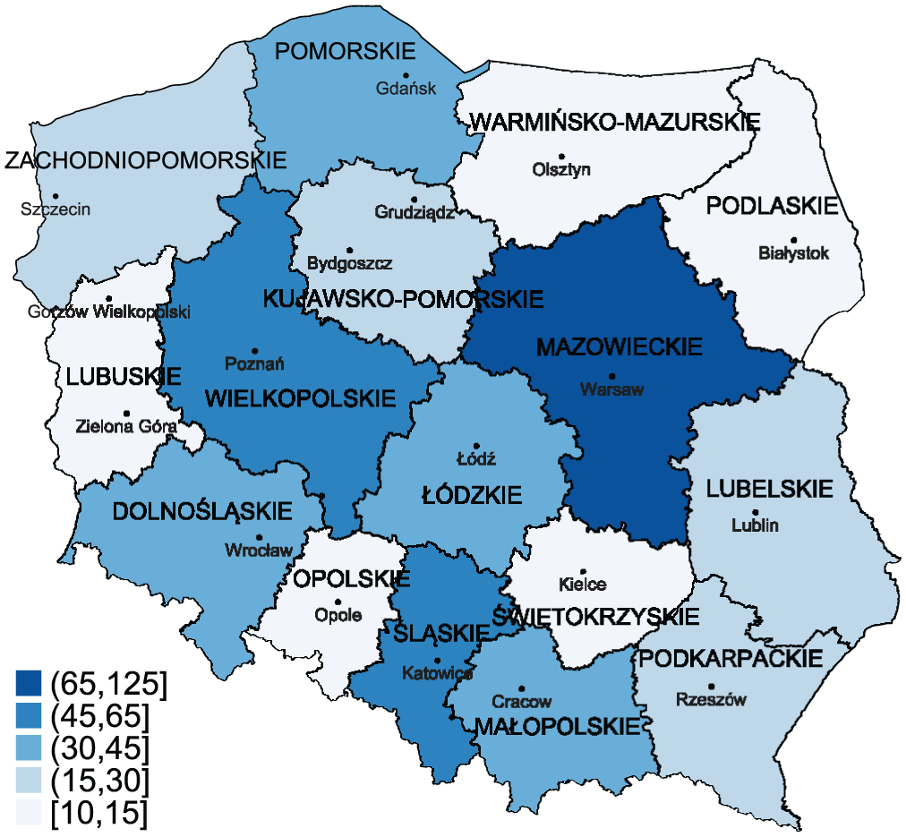
Nominal GDP for 2019 in Polish NUTS-2 regions (in billion EUR).
The calculations are conducted in Julia using the Ipopt solver. The codes and the data are available in GitHub repository at https://github.com/JanAcedanski/spatio-temporal-disaggregation-with-smoothing.
3.2. The Disaggregated Series for Polish Regions
The results of the sequential smoothing disaggregation procedure are presented in Figure 2. It shows the y-o-y growth rates of the disaggregated series and the corresponding growth rates of the country-level and annual regional-level input data. The outcome series are characterized by substantial smoothness, although some local spikes governed by the national data are visible. The most obvious is the COVID-19 crash in Q2 2020. Other notable jumps occur at the turn of 2009 and 2010 and in Q4 2015.
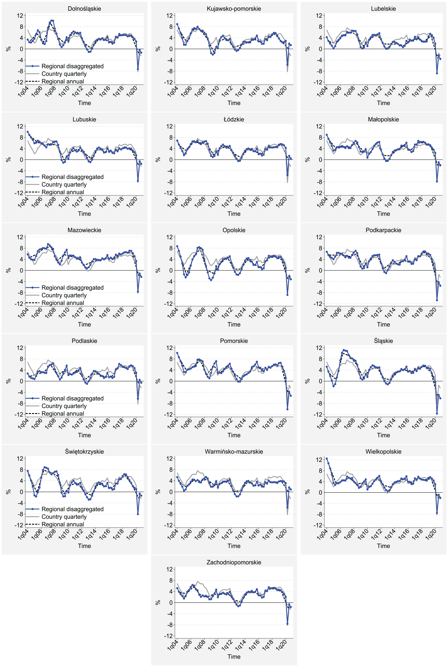
Disaggregation of real GDP series for Poland (y-o-y growth rates).
Table 1 presents the smoothness statistics for the disaggregated series. We use a simple version of the smoothness measure proposed by Froeb and Koyak (1994), defined as the ratio of the long-run standard deviation to the short-run one. The index is calculated as follows:
Smoothness Indices for the Disaggregated Series.
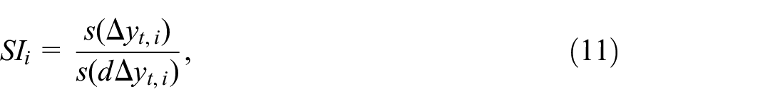
where
3.3. Comparison with the Alternative Approaches
In this subsection, we compare our baseline sequential smoothing disaggregation procedure with the two alternatives: the one-step version of the smoothing algorithm and the regression-based benchmarking method. The former approach relies on the same data as our baseline method. For the benchmarking method, we use four quarterly regional indicators as regressors. These are annual growth rates of: sold industrial production at constant prices, investment outlays, gross salary, and the consumer price index. The two middle series are deflated using the regional CPI indexes. Besides the unemployment rate that lags the business cycle considerably, these are the only Polish regional series available at the quarterly frequency for a longer period, starting from 2006. Because the industrial production series contain many outliers, we replace the annual growth rates that exceed 40% or are lower than −40% with the means of the neighborhood values. The distributions of the auxiliary regressors are shown in Figure 3.
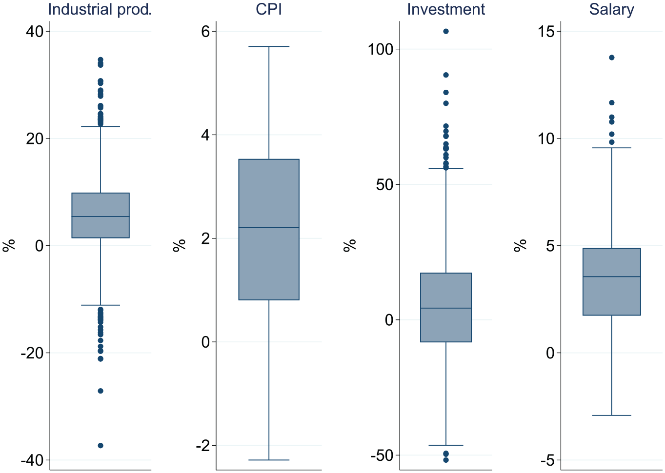
Distribution of the annual growth rates of the regressors used in the Chow-Lin method.
We use several distance measures between our baseline sequential smoothing procedure and the two alternatives. These are the mean difference (MD), mean absolute difference (MAD), and root mean square difference (RMSD), defined as:
where
In addition to the annual growth rates (y-o-y) reported above, we calculate the quarter-over-quarter (q-o-q) changes using the seasonally adjusted disaggregated series. For seasonal adjustments, we employ the default X-13ARIMA-SEATS procedure (Sax and Eddelbuettel 2018).
All the distance measures are calculated region-wise. In Table 2, we report the mean and extreme values of the measures across the regions.
The Differences Between the Sequential Smoothing Procedure and the Alternative Methods.
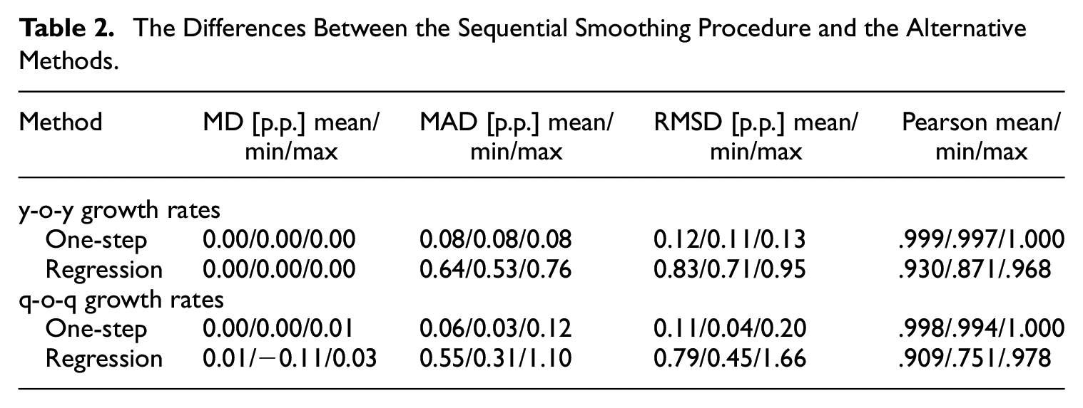
The differences between the sequential and one-step versions of the smoothing procedure are minimal. On average, the disaggregated series obtained from both methods coincide. The mean absolute difference for the annual growth rates slightly exceeds 0.1 p.p. on average, but it never reaches 0.2 p.p. The two series are also perfectly correlated, as the correlation coefficients never drop below .996. These results clearly show that the more practical sequential procedure can replace the one-step smoothing approach with minimal risk of result distortion.
Significantly higher differences are observed in the case of the regression-based procedure. Although the mean difference is also 0, the absolute and squared differences reach 0.6 p.p. and 0.8 p.p., on average, and 0.8 p.p. and 1.0 p.p., at most, respectively, for y-o-y growth series. In addition, although high, the correlation is far from perfect. The differences are quite similar for q-o-q growth rates.
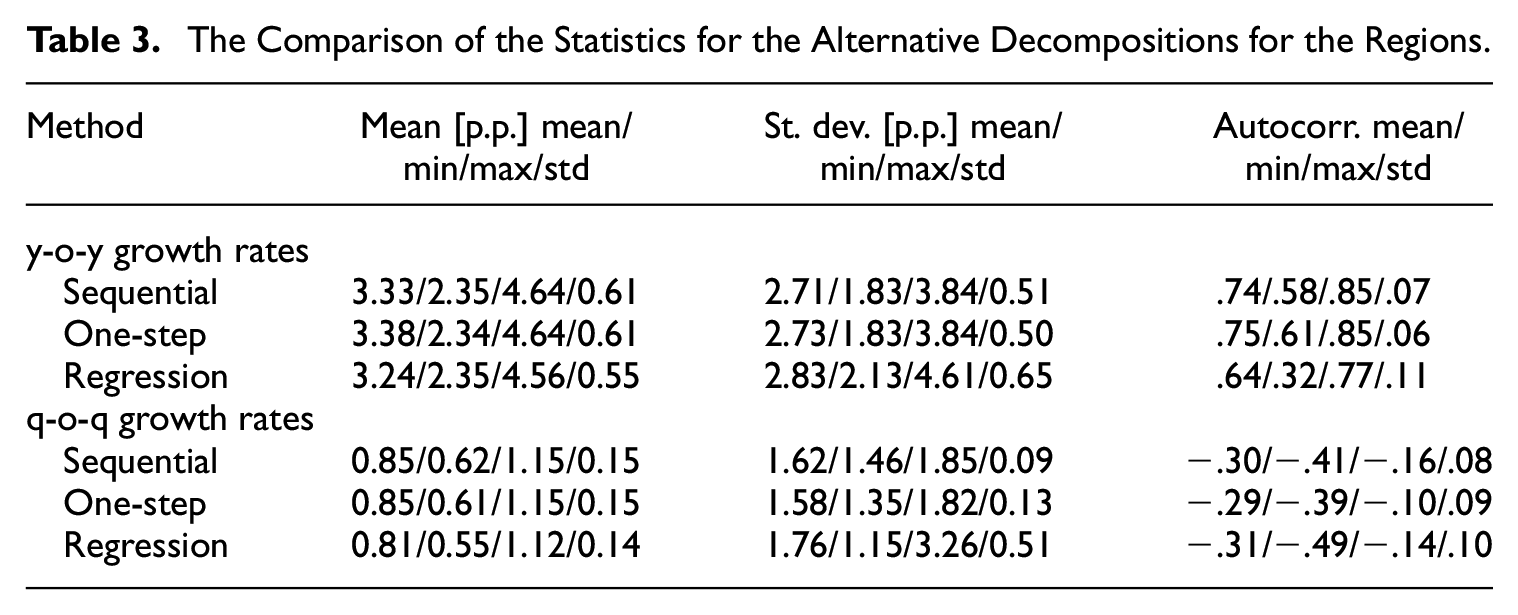
The differences between the sequential and regression-based procedures become less important when comparing the descriptive statistics of the two series, as shown in Table 3. For each region, we calculate means, standard deviations, and autocorrelations. The table reports the cross-sectional means, extremes, and standard deviations. Our baseline approach is characterized by marginally higher means (3.33 and 3.24 p.p. for y-o-y growth rates) for the disaggregated series and considerably lower volatility for some regions (see Figure 4). This is documented by the difference in serial standard deviations for the regions with the highest fluctuations of the disaggregated series (3.8 p.p. for sequential smoothing and 4.6 p.p. for the regression-based method) as well as the higher autocorrelations (.74 and .64, respectively).
The Comparison of the Statistics for the Alternative Decompositions for the Regions.
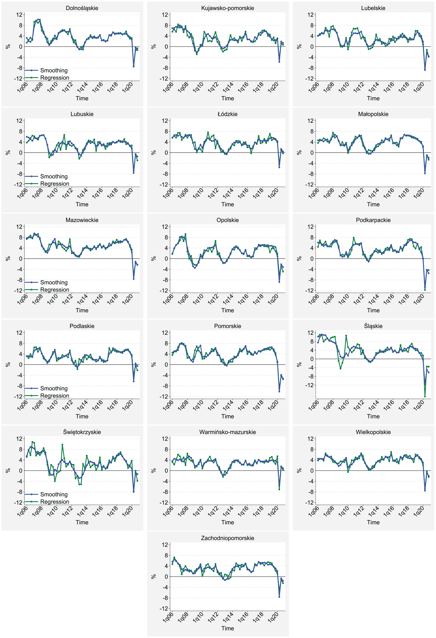
Comparison of the disaggregated series obtained from the smoothing and the regression-based procedures.
The ragged parts of the series disaggregated using the benchmarking procedure are shown in Figure 4. For example, they are visible for the 2010 to 2014 period in the case of some smaller regions, such as Kujawsko-Pomorskie, Lubuskie, Podlaskie, and, particularly, Świętokrzyskie. These jumps are likely to result from the poor quality of the regressors for these regions.
3.4. Differences in Business Cycle Dating
GDP series are frequently used for business cycle dating. While precise dating procedures go well beyond the GDP series, one of the most popular rules for identifying a recession involves determining a period of two consecutive quarters of decline in real GDP. We use this rule to compare recession dating based on q-o-q data from our sequential procedure and the regression-based alternative.
The results are shown in Table 4. It should be noted that Poland did not experience a recession at the country level in the investigated period. However, at the regional level, mild recessions were observed in 2008 to 2009, 2012 to 2013, and 2020 in some regions. The comparison presents mixed results. The highest consistency is observed for the COVID-19 crisis period, where both procedures give the same results (whether there was/was not a recession) for thirteen out of sixteen regions, including Śąskie region, where the recession had already started in Q4 2019. In addition, for the Global Financial Crisis period, the two procedures deliver the same outcome for thirteen regions, but the lengths and dating of the recession periods rather differ.
Recession Dating Based on the Smoothing and the Chow-Lin Procedures.

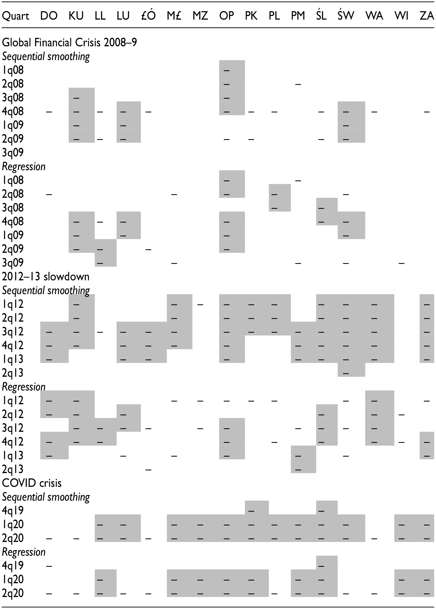
Note. The “minus” symbol indicates a quarter’s negative q-o-q growth rate. The shaded area represents a recession period defined as at least two consecutive negative growth rates.
However, a high level of disagreement is observed for the slowdown in 2012 to 2013. Sequential smoothing identifies recessions in thirteen regions with a median length of four quarters. The quarterly growth rates under the benchmarking procedure are much more scattered. As a result, recessions are identified in only nine regions.
4. Nowcasting Performance
In this section, we examine the nowcasting abilities of the smoothing algorithm and compare them with the performance of the regression-based method. For this purpose, we perform a pseudo-real time nowcasting experiment on the same Polish data as in the previous section. As a by-product of the experiment, we can also examine the size of the revisions resulting from the disaggregation of newly published annual regional data.
4.1. The Pseudo-Real-Time Nowcasting Experiment
We divide the whole dataset into eight extending samples. The first covers the period 2005 to 2011 and the last 2005 to 2018. For each sample, we first disaggregate the data solving the standard disaggregation problems Equation (6′)–(6″) and Equation (9). Given these disaggregated series, we calculate nowcasts for
More precisely, we solve eight different nowcasting problems and have eight sets of nowcasts obtained from the smoothing approach. This is because nowcasts for succeeding quarters are dependent, which means that adding a contemporaneous constraint for a new quarter and calculating the nowcasts for this period changes the previous periods’ nowcasts. The situation is different for the regression-based methods for which nowcasts are based on fixed regression coefficients and do not affect the previous estimates. As a result, to calculate the nowcasts for the next eight quarters, it suffices to solve the problem Equation (10) just once, taking
Notably, our forecasting experiment does not account for the official data revisions released in the studied period. We work on the latest available data published by Statistics Poland.
4.2. Measuring Nowcasting Performance
It is impossible to assess the accuracy of the obtained nowcasts objectively. Obviously, this is because the official quarterly, region-level GDP data are unavailable in Poland. To create the reference series for the accuracy assessment, we use the disaggregated data from the previous section obtained from the one-step smoothing procedure and the regression-based method calculated over the whole dataset. Then, we take the mean values of the two disaggregated series. The general conclusions remain valid even if we take only one of the disaggregated series, either smoothed or benchmarked, as the reference. The results for these cases are available upon request.
Given the reference series
where
4.3. Results
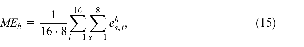
The values of the accuracy measures based on all eight samples are reported in Table 5. For shorter horizons, the smoothing algorithm delivers unbiased forecasts and slightly negatively biased for the longer ones, reaching −0.2 p.p. for
Nowcasting Accuracy—All Samples.
Also MAEs and RMSEs document the overall superiority of the smoothing method over the alternative approach, regardless of the horizon. The errors for the former are usually 30% to 75% smaller than for the latter.
The poor performance of the regression-based approach results from including extremely short samples in the analysis. Notably, the first one covers just six years of growth rates which means a single degree of freedom in the regression. Therefore, in Table 6, we study nowcasting abilities for different sample lengths.
Nowcast Accuracy for Different Sample Lengths.
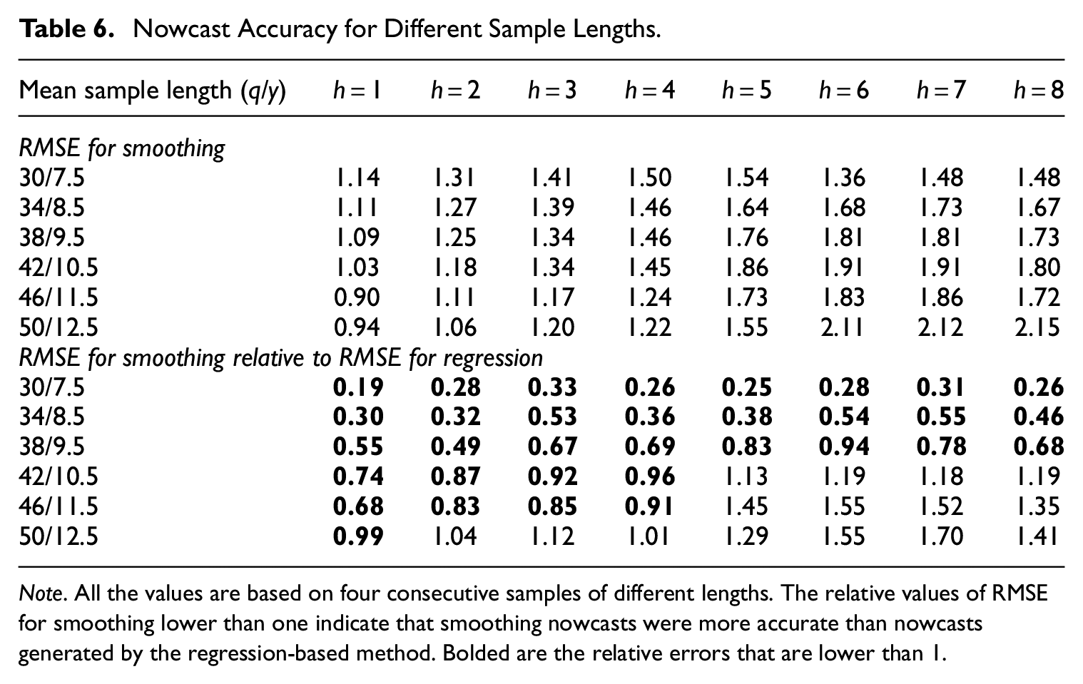
Note. All the values are based on four consecutive samples of different lengths. The relative values of RMSE for smoothing lower than one indicate that smoothing nowcasts were more accurate than nowcasts generated by the regression-based method. Bolded are the relative errors that are lower than 1.
The results show that the very short samples also decrease the accuracy of the smoothing method, but this effect is small and limited to horizons up to one year. For the longer horizons, the forecasts are more accurate for the short samples which is likely to be the result of sample composition.
The relative errors for smoothing reported in the bottom panel of Table 6 rise with the sample length confirming the increasing relative accuracy of the regression-based method. However, up to horizon of one year the smoothing method outperforms the alternative for all but the last sample lengths. For the longer horizons, the more accurate regression-based forecasts are observed even for shorter samples consisting of ten to eleven annual observations.
4.4. Quantification of the Revisions of the Disaggregated Series
Consecutive disaggregation of the extending samples in the nowcasting experiment allows for quantifying the revision size. Given eight samples, where the first one covers the period 2005 to 2011, we have eight series of growth rates of disaggregated series in the years 2006 to 2011 per method. The number of revisions decreases with time and in 2017, there are just two disaggregated series. To quantify the revision size, we consider two measures calculated annually: the mean standard deviation
where
The results are shown in Table 7. It documents that the revisions resulting from the regression-based method are substantial, and particularly huge before 2012. The mean standard deviations exceed one p.p., whereas the maximum revision considerably surpasses 30 p.p.. If we consider only the last five samples, the mean standard deviation for the Chow-Lin method drops considerably and never exceeds 0.15 p.p.. However, the maximum revisions can still be even higher than two p.p. On the other hand, even considering all the samples, the revisions for the sequential smoothing algorithm are small: the mean standard deviation never exceeds 0.08 p.p., and the maximum revision reaches 0.66 p.p. at most.
Size of the Revisions of the Disaggregated Series.
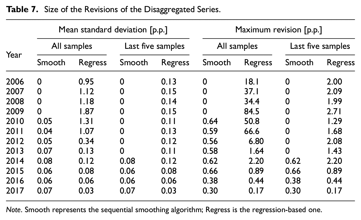
Note. Smooth represents the sequential smoothing algorithm; Regress is the regression-based one.
5. Discussion and Conclusion
This article proposes a novel spatiotemporal disaggregation method of economic time series. Our approach relies on the smoothing criterion and postulates that the annual growth rates of the disaggregated series should be as smooth as possible. Contrary to the existing methods, it is relatively simple, does not require auxiliary regressors, and is therefore well suited for statistical offices that lack long and reliable series of regional economic indicators, as well as disaggregation practices. We also show that the algorithm can be applied sequentially, which implies that one merely needs to revise the estimates for the last low-frequency period when new data are disaggregated. This is a useful feature when historical estimates are of interest, presenting another advantage over benchmarking algorithms.
Univariate temporal smoothing disaggregation methods are known to be subject to at least three serious weaknesses: the outcome series are overly smooth, the methods do not utilize available information, and they cannot be used for nowcasting and forecasting. As a result, this approach is commonly employed as a last resort (Eurostat 2013, 123).
These problems are considerably less severe in the multivariate version of the algorithm, as shown by the results presented in this study. In general, this is because of the country-level contemporaneous constraints that, to some extent, play the same role as the auxiliary regressors by guiding the nowcast values when the temporal regional constraints are unavailable.
As far as the excessive smoothness is concerned, the spatial contemporaneous constraints also restrict the space for smoothing, as shown by the short-run volatility visible in the disaggregated series. They are characterized by a similar level of smoothness as the country-level data. Nonetheless, this is still a sign of over-smoothness because the country-level aggregate, being a linear combination of the regional series, should, on average, be less volatile than its components.
Our study clearly shows that it is possible to nowcast with the multivariate smoothing method. The contemporaneous country-level constraints suffice to generate reasonable nowcasts. Moreover, in the case of short time series and poor quality of the regional business cycle benchmarks, accounting for the additional data does not necessarily lead to more accurate predictions.
We believe that one can merge smoothing with multivariate benchmarking, for example, by extending the linear regression objective function to include a smoothness-related term. It is likely to improve the nowcasting abilities of the regression-based methods in the case of the problematic data discussed in this study. However, we leave this problem for future research.
Footnotes
Acknowledgements
I am very grateful to anonymous reviewers and an associate editor for their detailed and insightful comments and suggestions, especially regarding the use of the interior point method. Their input has significantly enhanced the quality of the study. I also thank Marek A. Dąbrowski, Grzegorz Kończak, Jacek Osiewalski, Józef Pociecha, Andrzej Torój, and Aleksander Welfe for constructive comments on the earlier version of the study. All errors are entirely my own.
Funding
The author received no financial support for the research, authorship, and/or publication of this article.
Received: October 2022
Accepted: August 2024