Nowcasting in Triple-System Estimation

Abstract

Multiple systems estimation uses samples that each cover part of a population to obtain a total population size estimate. Ideally, all available samples are used, but if some samples are available (much) later, one may use only the samples that are available early. Under some regularity conditions, including sample independence, two samples are enough to obtain an asymptotically unbiased population size estimate. However, the assumption of sample independence may be unrealistic, especially when the samples are derived from administrative sources. The assumption of sample independence can be relaxed when using three or more samples, which is therefore generally recommended. This may be a problem if the third sample is available much later than the first two samples. Therefore, in this paper we propose a new approach that deals with this issue by utilizing older samples, using the so-called expectation maximization algorithm. This leads to a population size nowcast estimate that is asymptotically unbiased under more relaxed assumptions than the estimate based on two samples. The resulting nowcasting model is applied to the problem of estimating the number of homeless people in The Netherlands, leading to reasonably accurate nowcast estimates.

1. Introduction

A well-known problem in statistics production is that data may become available gradually, while it may be desirable to produce this statistic before all data are available. In such cases, it is common practice to produce a preliminary statistic that is based on some part of the data that is available early and update this statistic when all the data are available. Such a preliminary statistic, which has a widespread tradition that started mainly in time series analyses in economic literature, is often referred to as a “nowcast” estimate (see e.g., Giannone et al. 2006; Stundziene et al. 2024). The main idea is usually that the accuracy and reliability of a preliminary estimate may be improved by using historic data to estimate trends and cycles that should be taken into account. Discussion may also evolve around correcting for response bias that occurs when the speed of response is related to the statistic itself. For example, if companies with a rapidly growing turnover also respond quickly, a nowcast on turnover growth might be biased upward if this relation is ignored (see e.g., Zult, Krieg, et al. 2023). Other examples of nowcast estimation in the domain of official statistics or public policy can be found in for example, Equiza-Goñi (2022), van den Brakel and Michiels (2021), and Vanella et al. (2021).

A statistic for which such a nowcasting method is not available is a population size estimate that is based on samples that each partly observe a population, and some of these (complete) samples are available with delay. This may occur when, for example, samples are registers or surveys that are maintained or collected periodically throughout a certain period, where the statistician has little control over the data collection process. Then, some samples might be available early and others later. In such cases, it is common practice to simply wait until all samples have become available before estimation is performed. This raises the question whether and under what conditions it is possible to produce a preliminary population size estimate based on the set of samples that are available earlier. The simplest case is where one sample becomes available early and a second sample becomes available later. However, when these two samples are not independent, which is often the case when samples are derived from administrative sources, more than two samples are required to obtain an asymptotically unbiased population size estimate. This brings us to the more complex case, and the main topic of this paper, what if three samples become available sequentially and a statistic needs to be produced after the first or second sample becomes available?

The models that are involved in the estimation of the size of a partly observed population are known under different names such as capture-recapture, mark and recapture, or multiple systems estimation (MSE). When the number of samples is two, MSE is usually referred to as dual-system estimation (DSE) and when the number of samples is three, triple-system estimation (TSE). The most basic DSE model was proposed by Petersen (1896), and later by Lincoln (1930). Under a set of assumptions discussed by Wolter (1986), a DSE estimator provides an asymptotically unbiased population size estimate. When samples are derived from administrative sources, two of these assumptions become problematic. The first is the DSE assumption of homogeneous inclusion probabilities in at least one sample (see e.g., Seber 1982; van der Heijden et al. 2012), which can be somewhat relaxed when individual background variables/covariates (e.g., gender, age, etc.), that are related to inclusion probabilities, can be included in the model. The second problematic DSE assumption is the assumption of sample independence, which can be relaxed when three or more samples are included in the model (see Subsection 2.1 and 2.2 for further details). This implies that if samples are derived from administrative sources, TSE is generally recommended over DSE.

The basics of TSE are discussed in Fienberg (1972), and it has a long history in informing public policy (see e.g., Bird and King 2018, for an extensive discussion). For further technical discussions and applications of TSE with administrative data, see for example, Baffour et al. (2013, 2021) and Gerritse et al. (2016), who apply TSE to estimate the size of an unobserved part of a population in case of census or register data, or see van der Heijden et al. (2021) for an MSE application with four samples, including the population census, to estimate the size of the Māori population in New Zealand.

The case considered in this paper is that of a contingency table based on three samples for the previous period, and a contingency table based on one or two samples for the current period is available. The goal is to obtain a maximum likelihood (ML) population size estimate for the current period. The absence of a second and third, or only a third sample, for the current period could be considered a missing or incomplete data problem. A standard method to deal with incomplete data is the expectation–maximization (EM) algorithm (Dempster et al. 1977). The EM algorithm method allows for statistical inference from incomplete data with ML. In this paper we will discuss under which conditions the EM algorithm can be combined with DSE and TSE to obtain an asymptotically unbiased population size nowcast (NC) estimate. This approach of combining the EM algorithm with MSE models based on incomplete data is not new. For example, Zwane et al. (2004) consider the case that some samples may contain different but overlapping populations, Zwane and van der Heijden (2007) consider the case where some covariates are missing in some samples, and van der Heijden et al. (2021) who applies MSE and uses the EM algorithm to complete some missing data. New in this study is that the method is applied to obtain nowcasts for which both observations and estimates based on fully observed MSE data become available later. This allows us to compare the nowcasting model estimates with actual observations and estimates that are based on fully observed MSE data in a practical example.

Next, Section 2 discusses some basics of the DSE and TSE model, and how data for two periods can be combined in one framework. Section 3 discusses how the EM algorithm can be used to obtain ML estimates within this framework with incomplete data. The combination of DSE and TSE models and the EM algorithm, leads to our proposed MSE nowcasting model. Finally, in Section 4 the nowcasting model is applied to obtain NC estimates for the number of homeless people in The Netherlands. These NC estimates are compared with alternative estimates such as standard DSE estimates.

2. Theory and Notation

This section discusses DSE and TSE notation and theory, and shows how DSE and TSE models can be combined over two periods.

2.1. Dual-System Estimation

Imagine a population with size $N$ and a set of two samples $A$ and $B$ that each cover part of this population. The goal is to use these samples to obtain a population size estimate denoted as $\hat{N}$ . When each unit in each sample can be uniquely identified, then for each unit an inclusion pattern $\mathrm{ab}$ can be constructed, with $a,b\in \{0,1\}$ , where $a=0$ stands for “not included in sample”A′ and $a=1$ for “included in sample $A\prime$ ,” and the same with $b$ for sample $B$ . The units of each inclusion pattern can be counted and denoted as $n_{\mathrm{ab}}$ , except when the inclusion pattern is $00$ , because these units are unobserved. The sum of all observed units is denoted as $n$ and so $n=n_{11}+n_{10}+n_{01}$ . Finally, when we sum over $a$ or $b$ , we replace that subscript by a “+”. Thus, for example, $n_{1+}=n_{10}+n_{11}$ is equal to the size of source $A$ . It is assumed that $n_{\mathrm{ab}}$ is a realization of a random variable with expectation $m_{\mathrm{ab}}$ and the aim of DSE is to obtain ${\hat{m}}_{\mathrm{ab}}$ , an estimate of this expectation.

Under a set of assumptions discussed by for example, Wolter (1986), the observed counts $n_{11}$ , $n_{10}$ and $n_{01}$ can be used to estimate $N$ . These assumptions can be summarized as:

1. The sampling population is equal for samples $A$ and $B$ .

2. Records that correspond to the same unit in samples $A$ and $B$ can be perfectly linked.

3. Inclusion probabilities are homogeneous in samples $A$ or $B$ (see e.g., Seber 1982).

4. Samples $A$ and $B$ are independent.

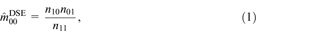
Under assumptions (1–4), an asymptotically unbiased DSE-estimator for $m_{00}$ can be written as

$${\hat{m}}_{00}^{\mathrm{DSE}}=\frac{n_{10}{n}_{01}}{n_{11}},$$

(1)

and consequently for $N$ as ${\hat{N}}^{\mathrm{DSE}}=n+{\hat{m}}_{00}^{\mathrm{DSE}}=\frac{n_{1+}{n}_{+1}}{n_{11}}$ .

Fienberg (1972) showed that the DSE estimator can also be derived from a log-linear model for $m_{\mathrm{ab}}$ , and for our purpose it is important to show how this relates to the independence assumption 4. A log-linear model for $m_{\mathrm{ab}}$ can be written as

$$\log m_{\mathrm{ab}}=\lambda +{\lambda }_a^A+{\lambda }_b^B+{\lambda }_{\mathrm{ab}}^{\mathrm{AB}},$$

(2)

with $\lambda$ an intercept term, ${\lambda }_a^A$ and ${\lambda }_b^B$ are the respective inclusion parameters for samples $A$ and $B$ that are identified by setting ${\lambda }_0^A={\lambda }_0^B=0$ and ${\lambda }_{\mathrm{ab}}^{\mathrm{AB}}$ is a parameter for the interaction between samples $A$ and $B$ . Because $m_{00}$ is unobserved and the independence assumption 4 implies that ${\lambda }_{\mathrm{ab}}^{\mathrm{AB}}=0$ , in practice the expectations $m_{\mathrm{ab}}$ are replaced with the observed counts/their ML estimates $n_{\mathrm{ab}}$ after which Equation (2) represents three equations and three unknowns that lead to the DSE-estimator in Equation (1). This also shows that if ${\lambda }_{\mathrm{ab}}^{\mathrm{AB}}\ne 0$ , then ${\hat{m}}_{00}^{\mathrm{DSE}}$ is a biased estimate for $m_{00}$ . In the next section we will show how TSE may solve this problem of bias due to pairwise dependence of samples.

2.2. Triple-System Estimation

When instead of being observed by two samples, a population is partly observed by three samples $A$ , $B$ , and $C$ , each unit has an inclusion pattern that, instead of $\mathrm{ab}$ , can be written as $\mathrm{abc}$ , where $c$ is defined in the same way as $a$ and $b$ . This means that instead of the four inclusion patterns in DSE there are now eight TSE inclusion patterns $000$ , $100$ , $010$ , $001$ , $110$ , $101$ , $011$ , and $111$ , and Equation (2) can be extended toward

$$\log m_{\mathrm{abc}}=\mu +{\mu }_a^A+{\mu }_b^B+{\mu }_c^C+{\mu }_{\mathrm{ab}}^{\mathrm{AB}}+{\mu }_{\mathrm{ac}}^{\mathrm{AC}}+{\mu }_{\mathrm{bc}}^{\mathrm{BC}}+{\mu }_{\mathrm{abc}}^{\mathrm{ABC}}.$$

(3)

Equation (3) is the three-sample representation of Equation (2), with $\mu$ the intercept, ${\mu }_a^A$ , ${\mu }_b^B$ , and ${\mu }_c^C$ the inclusion parameters, ${\mu }_{\mathrm{ab}}^{\mathrm{AB}}$ , ${\mu }_{\mathrm{ac}}^{\mathrm{AC}}$ , and ${\mu }_{\mathrm{bc}}^{\mathrm{BC}}$ the pairwise interaction parameters and ${\mu }_{\mathrm{abc}}^{\mathrm{ABC}}$ a three-way interaction parameter. It constitutes a system of eight linear equations and eight unknowns, but because $n_{000}$ is unobserved, it cannot be solved when $m_{\mathrm{abc}}$ are replaced by the observed counts/their ML estimates $n_{\mathrm{abc}}$ . Therefore it is usually assumed that ${\mu }_{\mathrm{abc}}^{\mathrm{ABC}}=0$ , which is similar to DSE assumption 4 but more realistic. This assumption gives the so-called saturated TSE model

$$\mathrm{saturated}:\log m_{\mathrm{abc}}=\mu +{\mu }_a^A+{\mu }_b^B+{\mu }_c^C+{\mu }_{\mathrm{ab}}^{\mathrm{AB}}+{\mu }_{\mathrm{ac}}^{\mathrm{AC}}+{\mu }_{\mathrm{bc}}^{\mathrm{BC}},$$

(4)

that in contrast to DSE, also cont(2022). Real-time mortality statistics during the covid-19 pandemic: A proposal ains pairwise interaction parameters ${\mu }_{\mathrm{ab}}^{\mathrm{AB}}$ , ${\mu }_{\mathrm{ac}}^{\mathrm{AC}}$ , and ${\mu }_{\mathrm{bc}}^{\mathrm{BC}}$ .

This model can be further restricted by setting one or more pairwise interaction terms to zero, which gives seven additional models, that is,

$$\mathrm{two}\mathrm{-}\mathrm{pair}\mathrm{dependence}(\mathrm{I}):\log m_{\mathrm{abc}}=\mu +{\mu }_a^A+{\mu }_b^B+{\mu }_c^C+{\mu }_{\mathrm{ac}}^{\mathrm{AC}}+{\mu }_{\mathrm{bc}}^{\mathrm{BC}},$$

(5)

$$\mathrm{two}\mathrm{-}\mathrm{pair}\mathrm{dependence}(\mathrm{II}):\log m_{\mathrm{abc}}=\mu +{\mu }_a^A+{\mu }_b^B+{\mu }_c^C+{\mu }_{\mathrm{ab}}^{\mathrm{AB}}+{\mu }_{\mathrm{bc}}^{\mathrm{BC}},$$

(6)

$$\mathrm{two}\mathrm{-}\mathrm{pair}\mathrm{dependence}(\mathrm{III}):\log m_{\mathrm{abc}}=\mu +{\mu }_a^A+{\mu }_b^B+{\mu }_c^C+{\mu }_{\mathrm{ab}}^{\mathrm{AB}}+{\mu }_{\mathrm{bc}}^{\mathrm{AC}},$$

(7)

$$\mathrm{one}\mathrm{-}\mathrm{pair}\mathrm{dependence}(\mathrm{I}):\log m_{\mathrm{abc}}=\mu +{\mu }_a^A+{\mu }_b^B+{\mu }_c^C+{\mu }_{\mathrm{bc}}^{\mathrm{BC}},$$

(8)

$$\mathrm{one}\mathrm{-}\mathrm{pair}\mathrm{dependence}(\mathrm{II}):\log m_{\mathrm{abc}}=\mu +{\mu }_a^A+{\mu }_b^B+{\mu }_c^C+{\mu }_{\mathrm{ac}}^{\mathrm{AC}},$$

(9)

$$\mathrm{one}\mathrm{-}\mathrm{pair}\mathrm{dependence}(\mathrm{III}):\log m_{\mathrm{abc}}=\mu +{\mu }_a^A+{\mu }_b^B+{\mu }_c^C+{\mu }_{\mathrm{ab}}^{\mathrm{AB}},$$

(10)

$$\mathrm{independence}:\log m_{\mathrm{abc}}=\mu +{\mu }_a^A+{\mu }_b^B+{\mu }_c^C.$$

(11)

Models with more than three samples can be developed along the same lines. For an extensive discussion of the models in Equations (4) to (11), we refer to Fienberg (1972) and Bishop et al. (1975), who also discuss derivations of closed form expressions or approximations for ${\hat{N}}^{\mathrm{TSE}}$ together with asymptotic variances, for each of these models. The distinction between the different restricted models is important when TSE and DSE over two periods are combined. This will be discussed in the next section.

2.3. Combining Samples Over Two Periods

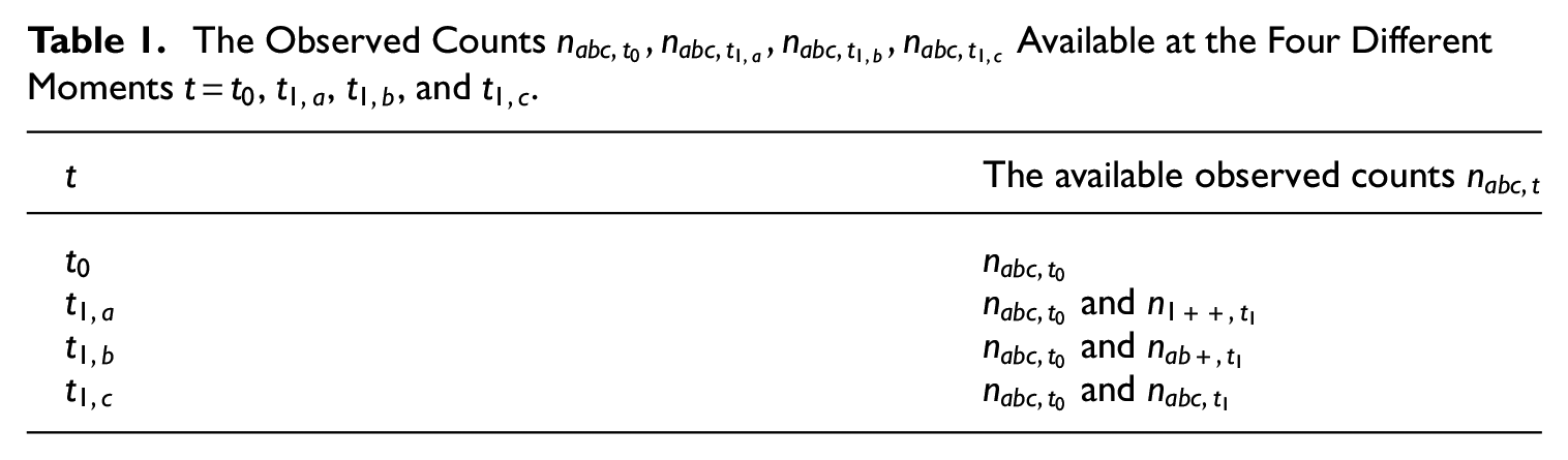
We consider a population with size $N_t$ and the samples $A_t$ , $B_t$ , and $C_t$ that each cover parts of this population for time $t$ . Also assume the delivery dates $t=t_0,t_{1,a},t_{1,b},t_{1,c}$ where at $t_0$ the samples $A_{t_0}$ , $B_{t_0}$ , and $C_{t_0}$ for time $t=t_0$ are available and at delivery dates $t_{1,a},t_{1,b}$ , and $t_{1,c}$ the samples $A_{t_1}$ , $B_{t_1}$ , and $C_{t_1}$ for time $t=t_1$ become available, one-by-one, in that order. This means that at both $t=t_0$ and $t=t_{1,c}$ three samples are available for their corresponding periods $t_0$ and $t_1$ . When we write $\mathrm{abc},t$ as the inclusion pattern for time $t$ , a table can be constructed that shows which observed counts are available at which moment, as in Table 1 below.

Table 1.

The Observed Counts $n_{\mathrm{abc},t_0},n_{\mathrm{abc},t_{1,a}},n_{\mathrm{abc},t_{1,b}},n_{\mathrm{abc},t_{1,c}}$ Available at the Four Different Moments $t=t_0$ , $t_{1,a}$ , $t_{1,b}$ , and $t_{1,c}$ .

$t$	The available observed counts $n_{\mathrm{abc},t}$
$t_0$	$n_{\mathrm{abc},t_0}$
$t_{1,a}$	$n_{\mathrm{abc},t_0}$ and $n_{1++,t_1}$
$t_{1,b}$	$n_{\mathrm{abc},t_0}$ and $n_{\mathrm{ab}+,t_1}$
$t_{1,c}$	$n_{\mathrm{abc},t_0}$ and $n_{\mathrm{abc},t_1}$

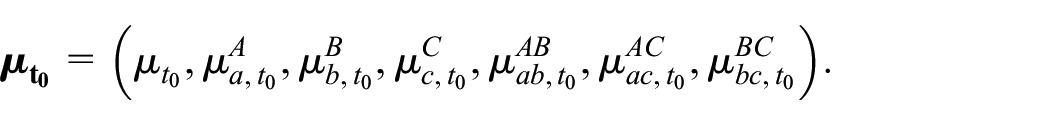
Table 1 shows that for $t=t_0$ and $t=t_{1,c}$ all observed counts are available for their corresponding periods, and so for each period a TSE-estimate for $m_{000,t}$ , as discussed in Subsection 2.2, can be estimated. We write their corresponding TSE models as $M_{t_0}\left({\mathbf{\mu }}_{t_0}\right)$ and $M_{t_{1,c}}({\mathbf{\mu }}_{t_{1,c}})=M_{t_1}\left({\mathbf{\mu }}_{t_1}\right)$ with ${\mathbf{\mu }}_t$ as the vector of ${\mu }_t$ -parameters at time $t$ . This gives, for example, for the saturated model in Equation (4) at $t=t_0$ , the set

$${\mathbf{\mu }}_{{\mathbf{t}}_0}=({\mu }_{t_0},{\mu }_{a,t_0}^A,{\mu }_{b,t_0}^B,{\mu }_{c,t_0}^C,{\mu }_{\mathrm{ab},t_0}^{\mathrm{AB}},{\mu }_{\mathrm{ac},t_0}^{\mathrm{AC}},{\mu }_{\mathrm{bc},t_0}^{\mathrm{BC}}).$$

(11)

At $t=t_{1,b}$ and $t=t_{1,a}$ it is not possible to apply TSE for $t=t_1$ , because at those delivery dates one or two samples are still missing. Table 1 shows that at those moments only aggregated observed counts are available. Then the question becomes if and under which assumptions, the old samples $A_{t_0}$ , $B_{t_0}$ , and $C_{t_0}$ , together with the aggregated observed counts for $t=t_1$ , can be used to obtain an asymptotically unbiased estimate for $N_{t_1}$ . In general, for each observed count that corresponds to a period $t$ , one additional parameter for that period can be estimated. This reasoning allows us to construct different MSE models based on the available samples at a given time.

At $t=t_{1,a}$ the additional observed count $n_{1++,t_1}$ becomes available, which simply is the total sample size of $A_{t_1}$ . This can be considered one observed count for time $t=t_1$ and therefore allows a model with one additional parameter for time $t=t_1$ , that is,

$$M_{t_{1,a}}({\mathbf{\mu }}_{{\mathit{t}}_{1\mathbf{,}\mathit{a}}})=\log m_{\mathrm{abc},t}=M_{t_0}({\mathbf{\mu }}_{{\mathit{t}}_{1\mathbf{,}\mathit{a}}})+{\mu }_{t_1},$$

(12)

with $M_{t_0}\left({\mathbf{\mu }}_{{\mathit{t}}_0}\right)$ as one of the models in Equations (4) to (11), but with a $t_0$ as subscript to the intercept parameter $\mu$ . This implies that in $M_{t_{1,a}}({\mathbf{\mu }}_{{\mathit{t}}_{1\mathbf{,}\mathit{a}}})$ , the intercept term may differ for $t=t_0$ and $t=t_1$ , but the inclusion and interaction parameters are equal for both periods. This means that for $m_{000,t_1}$ , Equation (12) reduces to the expression $m_{000,t_1}=\exp \left({\mu }_{t_1}\right)$ . This leads to an asymptotically unbiased estimate for $m_{000,t_1}$ and therefore $N_{t_1}$ if the estimated inclusion and interaction parameters are independent of $t$ .

At $t=t_{1,b}$ the additional sample $B_{t_1}$ becomes available and so at $t=t_{1,b}$ two samples are available for time $t=t_1$ . Table 1 shows that this means that three observed counts, with inclusion patterns $\mathrm{ab}+=11+,10+,01+$ , are available. This implies that for time $t=t_1$ a DSE-estimate can be obtained, but as was discussed in Subsection 2.1, this estimate is biased if the independence assumption is violated (i.e., if ${\lambda }_{\mathrm{ab}}^{\mathrm{AB}}\ne 0$ ). Then the question becomes if the presence of the samples $A_{t_0}$ , $B_{t_0}$ , and $C_{t_0}$ allows for a way in which the independence assumption can be relaxed. Note that due to the three observed counts we can extend $M_{t_{1,a}}({\mathbf{\mu }}_{{\mathbf{t}}_{1,\mathit{a}}})$ in Equation (12) with two additional parameters for $t=t_1$ , that is,

$$M_{{\mathit{t}}_{1,\mathit{b}}}({\mathbf{\mu }}_{{\mathit{t}}_{1,\mathit{b}}})=\log m_{\mathrm{abc},t}=M_{t_0}({\mathbf{\mu }}_{{\mathit{t}}_{1,\mathit{b}}})+{\mu }_{t_1}+{\mu }_{a,t_1}^A+{\mu }_{b,t_1}^B.$$

(13)

${\mathbf{\mu }}_{{\mathit{t}}_{1,\mathit{b}}}$ differs from the ${\mathbf{\mu }}_{{\mathit{t}}_{1\mathbf{,}\mathit{a}}}$ in Equation (12), because instead of the time independent parameters ${\mu }_a$ and ${\mu }_b$ , it contains the time dependent parameters ${\mu }_{a,t_0}$ and ${\mu }_{b,t_0}$ , which are just like ${\mu }_{t_0}$ equal to zero for $t=t_0$ . This model again gives the same expression $\exp ({\mu }_{t_1})$ , but the conditions under which the ML-estimator for the parameter ${\mu }_{t_1}$ is an asymptotically unbiased estimator are more relaxed. Note that the parameters in $M_{t_0}({\mathbf{\mu }}_{{\mathit{t}}_{1,\mathit{b}}})$ that should hold for both periods have reduced with the addition of ${\mu }_{a,t_0}^A$ and ${\mu }_{b,t_0}^B$ , which now, due to the presence of ${\mu }_{a,t_1}^A$ and ${\mu }_{b,t_1}^B$ , correspond exclusively to inclusion probabilities for time $t_0$ . Therefore, for model $M_{{\mathit{t}}_{1,\mathit{b}}}({\mathbf{\mu }}_{{\mathit{t}}_{1,\mathit{b}}})$ to hold, as compared to model $M_{t_{1,a}}({\mathbf{\mu }}_{{\mathit{t}}_{1\mathbf{,}\mathit{a}}})$ , only the inclusion parameter ${\mu }_c$ and the interaction parameters ${\mu }_{\mathrm{ab}}^{\mathrm{AB}}$ , ${\mu }_{\mathrm{ac}}^{\mathrm{AC}}$ , and ${\mu }_{\mathrm{bc}}^{\mathrm{BC}}$ should be independent of $t$ .

When $m_{\mathrm{abc},t}=m_{\mathrm{ab}}$ , ${\mu }_{t_1}=\lambda$ , ${\mu }_{a,t_1}^A={\lambda }_a^A$ , ${\mu }_{b,t_1}^B={\lambda }_b^B$ , and $M_{t_0}({\mathbf{\mu }}_{{\mathit{t}}_{1,\mathit{b}}})={\lambda }_{\mathrm{ab}}^{\mathrm{AB}}$ , the MSE model in Equation (13) and the DSE model in Equation (2) are equivalent. This implies that for $M_{{\mathit{t}}_{1,\mathit{b}}}({\mathbf{\mu }}_{{\mathit{t}}_{1,\mathit{b}}})$ the DSE independence assumption 4 can be replaced by the (more relaxed) assumption 4. The pairwise dependence parameter ${\lambda }_{\mathrm{ab}}^{\mathrm{AB}}$ is independent of $t$ .

In other words, the estimate for ${\lambda }_{\mathrm{ab}}^{\mathrm{AB}}={\mu }_c+{\mu }_{\mathrm{ab}}^{\mathrm{AB}}+{\mu }_{\mathrm{ac}}^{\mathrm{AC}}+{\mu }_{\mathrm{bc}}^{\mathrm{BC}}$ for the previous period, can be used as an estimate for the current period, because it is assumed to be stable between both periods.

The estimation of the parameters in the models $M_{t_{1,a}}({\mathbf{\mu }}_{{\mathit{t}}_{1\mathbf{,}\mathit{a}}})$ and $M_{t_{1,b}}({\mathbf{\mu }}_{{\mathit{t}}_{1,\mathit{b}}})$ is less straightforward than the estimation of the parameters in $M_{t_0}({\mathbf{\mu }}_{{\mathit{t}}_0})$ and $M_{t_1}({\mathbf{\mu }}_{{\mathit{t}}_1})$ , which can be estimated directly with ML. How to deal with this problem is discussed in the next section.

3. Combining DSE and TSE with the EM Algorithm

Table 1 from the previous section poses two statistical estimation problems. On top of the problem of the unobserved counts $n_{000,t_0}$ and $n_{000,t_1}$ , it also poses a so-called mixture model problem (see e.g., Lindsay 1995). This problem implies that for (some) variables only an aggregate over different groups is observed, or one may say that for some groups the data is incomplete. In this case, at $t=t_{1,a}$ , there is the aggregated observed count $n_{1++,t_1}$ and at $t=t_{1,b}$ there are the three aggregated observed counts $(n_{11+,t_1},n_{10+,t_1},n_{01+,t_1})$ . $n_{1++,t_1}$ is simply the size of sample $A_{t_1}$ , and $(n_{11+,t_1},n_{10+,t_1},n_{01+,t_1})$ are the aggregated observed counts over sample $C_{t_1}$ of the units included in sample $A_{t_1}$ and/or $B_{t_1}$ . A standard method to deal with incomplete data is the EM algorithm. In this case, it allows for the estimation of the underlying counts that together add up to the observed aggregated counts, such as the unobserved $n_{111,t_1}$ and $n_{110,t_1}$ at $t=t_{1,b}$ that add up to the observed $n_{11+,t_1}$ .

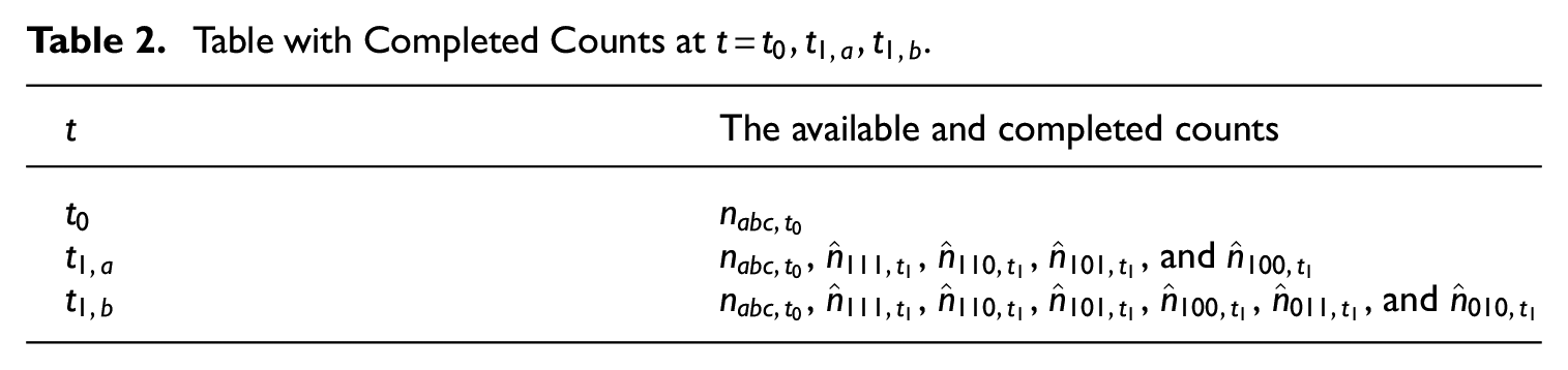
The EM algorithm was introduced by Dempster et al. (1977) as a tool to obtain ML-estimates in case of incomplete data due to unobserved or latent variables. In the problem discussed in this paper, the EM algorithm can be applied with model $M_{t_{1,a}}({\mathbf{\mu }}_{{\mathit{t}}_{1\mathbf{,}\mathit{a}}})$ or $M_{{\mathit{t}}_{1,\mathit{b}}}({\mathbf{\mu }}_{{\mathit{t}}_{1,\mathit{b}}})$ in Equations (12) and (13). This gives, based on the model for $t_0$ , an estimated split-up of the available frequencies at $t_1$ (e.g., $n_{1++,t_{1,a}}={\hat{n}}_{111,t_1}+{\hat{n}}_{110,t_1}+{\hat{n}}_{101,t_1}+{\hat{n}}_{100,t_1}$ ), which we refer to as completed counts. For this case, the result of the EM algorithm in $t=t_{t,a}$ and $t=t_{t,b}$ is shown in Table 2.

Table 2.

Table with Completed Counts at $t=t_0,t_{1,a},t_{1,b}$ .

$t$	The available and completed counts
$t_0$	$n_{\mathrm{abc},t_0}$
$t_{1,a}$	$n_{\mathrm{abc},t_0}$ , ${\hat{n}}_{111,t_1}$ , ${\hat{n}}_{110,t_1}$ , ${\hat{n}}_{101,t_1}$ , and ${\hat{n}}_{100,t_1}$
$t_{1,b}$	$n_{\mathrm{abc},t_0}$ , ${\hat{n}}_{111,t_1}$ , ${\hat{n}}_{110,t_1}$ , ${\hat{n}}_{101,t_1}$ , ${\hat{n}}_{100,t_1}$ , ${\hat{n}}_{011,t_1}$ , and ${\hat{n}}_{010,t_1}$

To illustrate how the Expectation step (E-step) of the EM algorithm yields completed data in the columns ${\hat{n}}_{\mathrm{abc},t_{1,a}}$ and ${\hat{n}}_{\mathrm{abc},t_{1,b}}$ in Table 2, we discuss this for ${\hat{n}}_{\mathrm{abc},t_{1,b}}$ . The EM algorithm allows one to split $n_{\mathrm{ab}+,t_1}$ into the completed data ${\hat{n}}_{\mathrm{ab}1,t_{1,b}}$ and ${\hat{n}}_{\mathrm{ab}0,t_{1,b}}$ with ${\hat{n}}_{\mathrm{ab}1,t_{1,b}}+{\hat{n}}_{\mathrm{ab}0,t_{1,b}}=n_{\mathrm{ab}+,t_1}$ . The EM algorithm starts with an initialization step that creates an initial set of completed data, for example, by ${\hat{n}}_{\mathrm{ab}1,t_{1,b}}^{(0)}=n_{\mathrm{ab}+,t_1}/2$ and ${\hat{n}}_{\mathrm{ab}0,t_{1,b}}^{(0)}=n_{\mathrm{ab}+,t_1}/2$ . Next, in the first maximization step (M-step) these completed data are assumed regular observations that, together with $n_{\mathrm{abc},t_0}$ , can be used to estimate the parameters of the model $M_{t_{1,b}}({\mathbf{\mu }}_{{\mathit{t}}_{1,\mathit{b}}})$ in Equation (13), but here it is also possible to replace $M_{t_0}({\mathbf{\mu }}_{{\mathit{t}}_0})$ with a more restricted model. The model resulting from this application of the EM algorithm gives, in iteration $0$ , the fitted values ${\hat{m}}_{\mathrm{abc},t}^{(0)}$ . Next, in the first expectation step (E-step) these fitted values are used to split-up $n_{\mathrm{ab}+,t_1}$ (again), but now as ${\hat{n}}_{\mathrm{ab}1,t_{1,b}}^{(1)}=n_{\mathrm{ab}+,t_1}({\hat{m}}_{\mathrm{ab}1,t_{1,b}}^{(0)}/{\hat{m}}_{\mathrm{ab}+,t_{1,b}}^{(0)}$ ) and ${\hat{n}}_{\mathrm{ab}0,t_{1,b}}^{(1)}=n_{\mathrm{ab}+,t_1}({\hat{m}}_{\mathrm{ab}0,t_{1,b}}^{(0)}/{\hat{m}}_{\mathrm{ab}+,t_{1,b}}^{(0)})$ , which gives a new set of completed data that can be used to, again, estimate the model in Equation (13). This iterative procedure repeats itself $i$ times until ${\hat{n}}_{\mathrm{abc},t_{1,b}}^{(i)}$ converges. The resulting set of completed stabilized data is ${\hat{n}}_{\mathrm{abc},t_{1,b}}$ in Table 2, and they are used to derive maximum likelihood estimates ${\hat{m}}_{\mathrm{abc},t_{1,b}}$ .

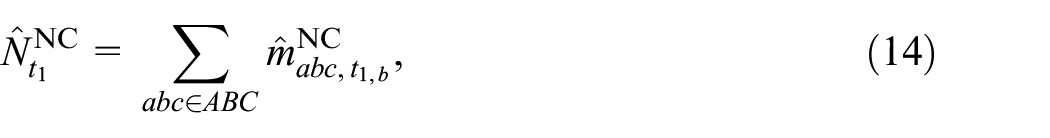
The last M-step provides fitted values ${\hat{m}}_{\mathrm{abc},t}$ for each cell, including the cells with inclusion patterns $001,t_1$ and $000,t_1$ . We refer to these estimates as ${\hat{m}}_{\mathrm{abc},t}^{\mathrm{NC}}$ and summing up over them for $t=t_{1,b}$ gives a fitted value for $N_{t_1}$ . We refer to this sum as the nowcast estimate for $N_{t_1}$ , that is,

$${\hat{N}}_{t_1}^{\mathrm{NC}}=\sum _{\mathrm{abc}\in \mathrm{ABC}}{\hat{m}}_{\mathrm{abc},t_{1,b}}^{\mathrm{NC}},$$

(14)

with $\mathrm{ABC}$ the set of all inclusion patterns. In the next section, we will use the estimator in Equation (14) to obtain nowcasts of the number of homeless people in The Netherlands.

A drawback of the EM algorithm, is that is it does not provide the asymptotic variance–covariance matrix (see e.g., Xu et al. 2014), so it seems not possible to derive an analytical expression for the variance of the NC-estimator in Equation (14)), such as for the regular DSE- and TSE-estimators (see e.g., Bishop et al. 1975, Ch. 6, for these expressions). An alternative way to construct confidence intervals for MSE-estimators, proposed by Buckland and Garthwaite (1991), is to construct confidence intervals with the bootstrap approach introduced by Efron (1979). For the example of homeless people in The Netherlands discussed in the next section, this approach was adopted in Coumans et al. (2017) and Zult, van der Heijden, and Bakker (2023).

4. Nowcasting the Number of Homeless People in The Netherlands

In this section, we investigate how the MSE nowcasting model performs by using a dataset that is also used to estimate the number of homeless people in The Netherlands, which is discussed in further detail in Coumans et al. (2017). The estimation procedure is performed annually and is based on three samples that are derived from administrative sources, and we refer to them as sample $A_y$ , $B_y$ , and $C_y$ , where $y$ indicates the year. The resulting TSE estimate for the $1^{\mathrm{st}}$ of January of each year is based on a model selection procedure that leads to a TSE model that also includes a set of covariates, namely gender, age, region of stay, and region of birth. These covariates are included in the model, because the MSE models discussed so far assume that inclusion probabilities are equal for everyone in at least one sample (see assumption 3 in Subsection 2.1). When this assumption is violated, because inclusion probabilities differ between groups, but these groups can be identified by covariates that are available, this violation can be controlled for by including these covariates in the model. For example, in The Netherlands younger men are more likely to be homeless than older women, and therefore a record in an administrative sample on homeless people in The Netherlands is more likely to be a younger man than an older woman, which violates assumption 3. By including the covariates gender and age, the difference in inclusion probabilities for these two groups can be controlled for by the model. See Alho (1990) for a more in-depth discussion on this topic. A more up-to-date time series of estimates of the number of homeless people in The Netherlands, together with their confidence intervals, is presented in Zult, van der Heijden, and Bakker (2023).

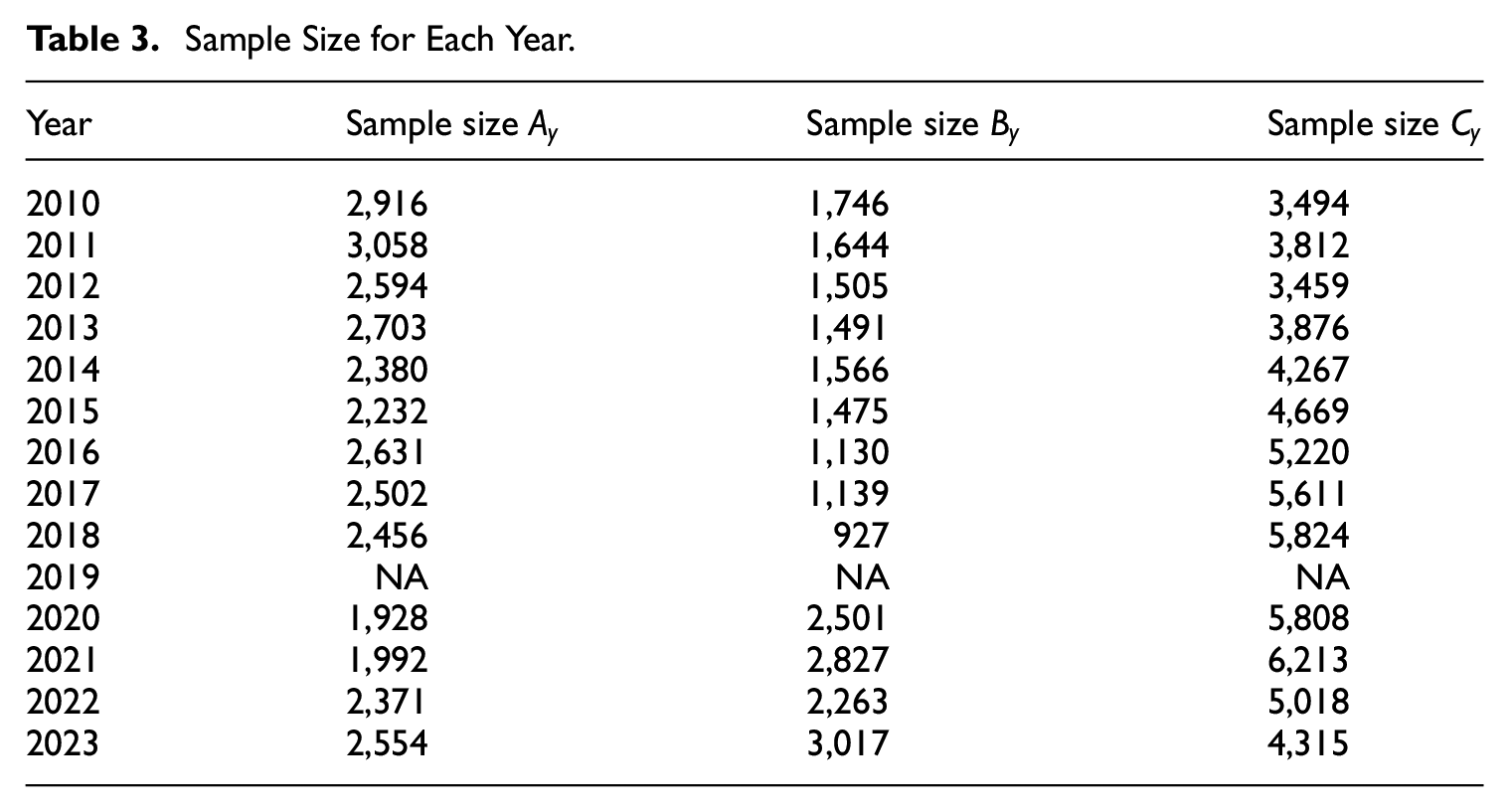
The samples used become available during the year, where the first two samples $A_y$ and $B_y$ are available early during the year, and the third sample $C_y$ becomes available sometime around the third or fourth quarter of the year. These samples are available for each year for the period $2010-2023$ , except for the year $2019$ . Therefore, in $2020$ , this sample was replaced with another sample from another administrative source. Because in $2019$ sample $B_y$ was missing, for that year the other two samples were also not processed and are therefore also unavailable. The sample size for each sample in each year is presented in Table 3 below.

Table 3.

Sample Size for Each Year.

Year	Sample size $A_y$	Sample size $B_y$	Sample size $C_y$
2010	2,916	1,746	3,494
2011	3,058	1,644	3,812
2012	2,594	1,505	3,459
2013	2,703	1,491	3,876
2014	2,380	1,566	4,267
2015	2,232	1,475	4,669
2016	2,631	1,130	5,220
2017	2,502	1,139	5,611
2018	2,456	927	5,824
2019	NA	NA	NA
2020	1,928	2,501	5,808
2021	1,992	2,827	6,213
2022	2,371	2,263	5,018
2023	2,554	3,017	4,315

The scheme in which the samples become available implies that at $y=y_{{\mathit{t}}_{1,\mathit{b}}},\mathrm{for}\mathrm{the}\mathrm{years}2011-2018$ and $2021-2023$ , both a DSE estimate and a NC estimate can be obtained. The fact that a NC estimate, as discussed in Section 2.3 and defined in Equation (14), requires samples from two consecutive years means that it cannot be calculated for the years $2010$ , $2019$ , and $2020$ , because in those years data for the previous or next year are missing.

To simplify the interpretability of the results, both the model selection procedure is simplified by assuming a saturated model, as defined in Equation (4), for model $M_{t_0}({\mathbf{\mu }}_{{\mathit{t}}_{1,\mathit{b}}})$ (see Equation (13)). Simply assuming the saturated model in Equation (4) for each period, allows for a more fair and straightforward comparison of the resulting estimates between periods. Also, the available covariates are removed from the model by aggregating over the observed frequencies for each covariate. So for example, instead of using the observed frequencies for men and women separately and using gender as an additional explanatory variable in the TSE model equation, the two frequencies are summed-up into one aggregated frequency and gender is left out of the TSE model equation. Aggregating over covariates simplifies the data to the data presented in Table 1 in Subsection 2.3.

To further increase the generality of the analysis, the order in which the samples become available is assumed to be possible in all possible orders. In reality sample $C_y$ is available last, but for analytical purposes the order of the samples can be switched without loss of generality. To indicate which samples are assumed to be available first, they are denoted in the subscript. For example, a NC estimate based on sample $A_{y-1}$ , $B_{y-1}$ , $C_{y-1}$ , $A_y$ , and $B_y$ , but not $C_y$ , is denoted as ${\hat{N}}_{\mathrm{ab},y}^{\mathrm{NC}}$ .

4.1. Results

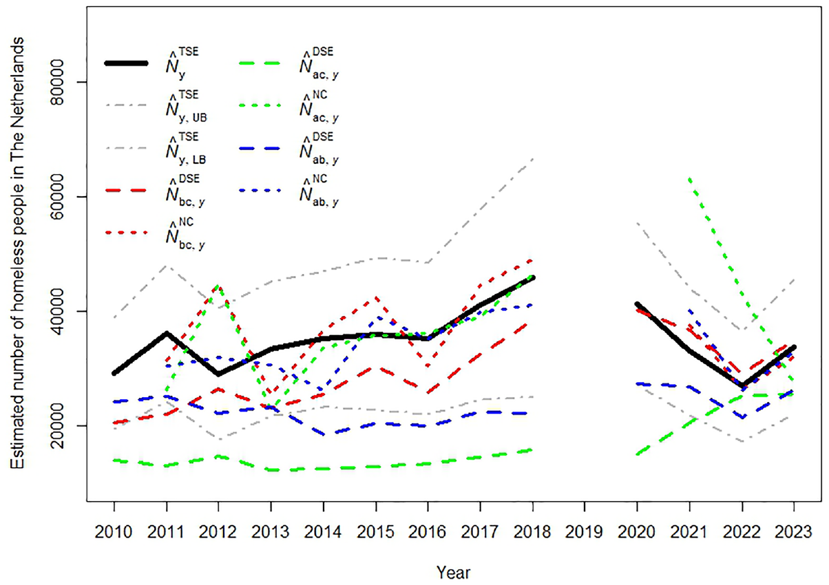
Figure 1 presents different time series of population size estimates. It presents the regular TSE estimates ${\hat{N}}_y^{\mathrm{TSE}}$ together with their 95% confidence interval indicated by ${\hat{N}}_{y,\mathrm{UB}}^{\mathrm{TSE}}$ and ${\hat{N}}_{y,\mathrm{LB}}^{\mathrm{TSE}}$ . This confidence interval is constructed by using the estimate for the asymptotic variance, for the saturated TSE model, given by Bishop et al. (1975, 242). Figure 1 also presents the regular DSE estimates ( ${\hat{N}}_{\mathrm{bc},y}^{\mathrm{DSE}}$ , ${\hat{N}}_{\mathrm{ac},y}^{\mathrm{DSE}}$ , and ${\hat{N}}_{\mathrm{ab},y}^{\mathrm{DSE}}$ ) and NC estimates ( ${\hat{N}}_{\mathrm{bc},y}^{\mathrm{NC}}$ , ${\hat{N}}_{\mathrm{ac},y}^{\mathrm{NC}}$ , and ${\hat{N}}_{\mathrm{ab},y}^{\mathrm{NC}}$ ) of the total population size for each year. The figure shows that for most years the NC estimates are closer to the regular TSE estimates than to the DSE estimates, which suggest that in this case the nowcasting model assumption of ${\lambda }_{\mathrm{ab},y}^{\mathrm{AB}}={\lambda }_{\mathrm{ab},(y-1)}^{\mathrm{AB}}$ is more reasonable than the DSE assumption ${\lambda }_{\mathrm{ab},y}^{\mathrm{AB}}=0$ . Furthermore, most NC estimates are within the confidence interval of the regular TSE estimates, while this is not the case for many DSE estimates, especially during the period $2010-2018$ . In particular the NC estimates ${\hat{N}}_{\mathrm{ab},y}^{\mathrm{NC}}$ represented by the blue (short-dotted) line, which represent the real situation, seems to perform reasonably well in most years. The red and green (short-dotted) line generally perform a bit less well, in particular the estimates ${\hat{N}}_{\mathrm{ac},y}^{\mathrm{NC}}$ for the years $2021$ and $2022$ are quite bad. Interestingly, although not shown here, these two outliers disappear when for $M_{t_0}({\mathbf{\mu }}_{{\mathit{t}}_{1,\mathit{b}}})$ , for the years $2021$ and $2022$ instead of the saturated model in Equation (4), the two-pair dependence model in Equation (5) is chosen. This suggests that by applying a well-designed model selection procedure in the nowcasting approach as in Coumans et al. (2017), which is not possible in DSE, the accuracy of the nowcasting estimates in Figure 1 can be further improved.

Figure 1.

Estimates of the number of the total number of homeless people in The Netherlands over the periods $2010-2018$ and $2020-2023$ .

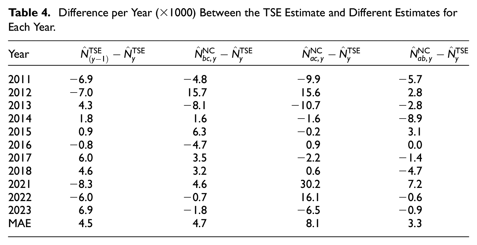
Figure 1 also shows that the lagged TSE estimates, that is, the TSE estimates of the previous year, are also within the TSE confidence intervals. This raises the question whether in this case it makes any sense to apply the nowcasting model. To look deeper into this issue, Table 4 presents the annual differences between the TSE estimates and the lagged TSE estimates (presented in the column ${\hat{N}}_{(y-1)}^{\mathrm{TSE}}-{\hat{N}}_y^{\mathrm{TSE}}$ ), together with the annual differences between the TSE estimates and the three different NC estimates. Table 4 shows that the differences between NC estimates and TSE estimates clearly differ for each sample order. The best results are in the last column ${\hat{N}}_{\mathrm{ab},y}^{\mathrm{NC}}-{\hat{N}}_y^{\mathrm{TSE}}$ , which has the lowest mean absolute error (MAE, $3.3$ ) and implies that in the case of the homeless data the nowcasting model with sample $C_y$ being later (which corresponds to the real situation), gives the best nowcasting results that are also slightly more accurate than the lagged TSE estimates. To further compare the predictive accuracy of the lagged TSE estimate and the three NC estimates, we also apply the Diebold-Mariano test (Diebold and Mariano 1995), which can be used to tests for statistical differences in predictive accuracy of different series. For the 95% confidence level, this test does not reject statistically significant differences in predictive accuracy between the four different series, which may also be due to the limited number of estimates over time.

Table 4.

Difference per Year ( $\times 1000$ ) Between the TSE Estimate and Different Estimates for Each Year.

Year	${\hat{N}}_{(y-1)}^{\mathrm{TSE}}-{\hat{N}}_y^{\mathrm{TSE}}$	${\hat{N}}_{\mathrm{bc},y}^{\mathrm{NC}}-{\hat{N}}_y^{\mathrm{TSE}}$	${\hat{N}}_{\mathrm{ac},y}^{\mathrm{NC}}-{\hat{N}}_y^{\mathrm{TSE}}$	${\hat{N}}_{\mathrm{ab},y}^{\mathrm{NC}}-{\hat{N}}_y^{\mathrm{TSE}}$
2011	−6.9	−4.8	−9.9	−5.7
2012	−7.0	15.7	15.6	2.8
2013	4.3	−8.1	−10.7	−2.8
2014	1.8	1.6	−1.6	−8.9
2015	0.9	6.3	−0.2	3.1
2016	−0.8	−4.7	0.9	0.0
2017	6.0	3.5	−2.2	−1.4
2018	4.6	3.2	0.6	−4.7
2021	−8.3	4.6	30.2	7.2
2022	−6.0	−0.7	16.1	−0.6
2023	6.9	−1.8	−6.5	−0.9
MAE	4.5	4.7	8.1	3.3

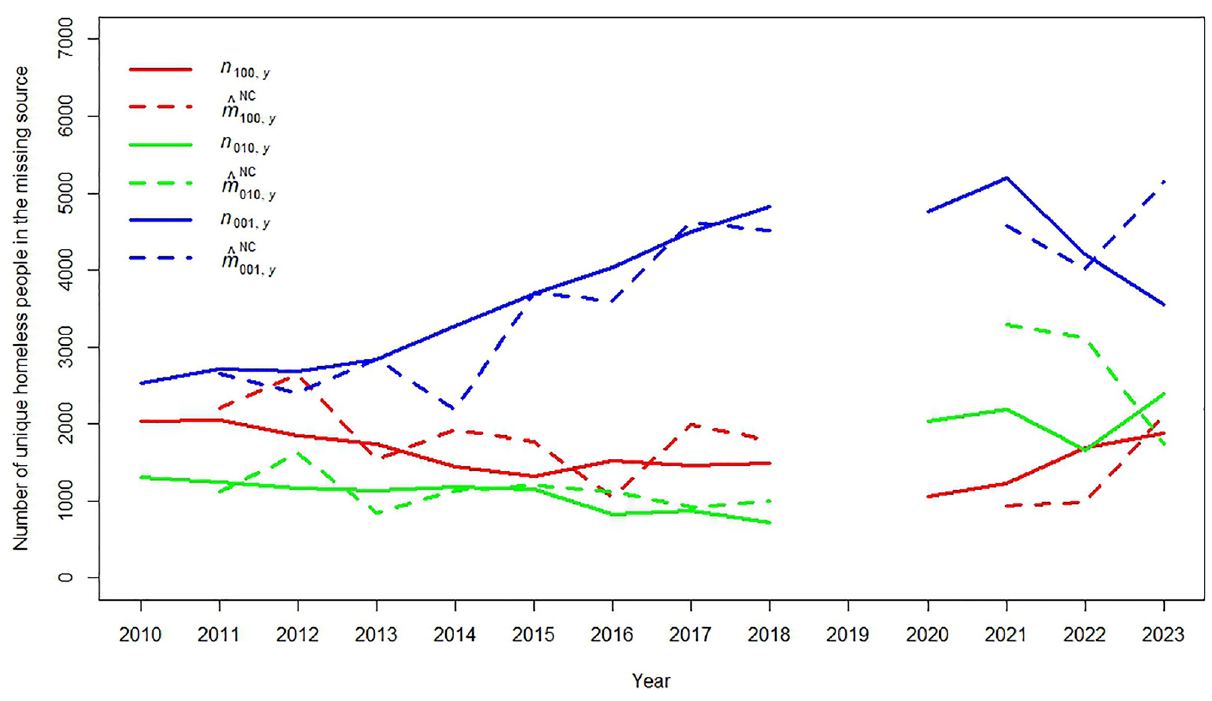
An advantage that is common to nowcasting models that can also be utilized in the study presented in this section, is that NC estimates can often be compared with true values that become available later. In most MSE applications such an evaluation is not possible, simply because the true population size usually remains unknown. However, in this study the nowcasting model, additional to the NC estimate for the total population, it also provides a NC estimate ${\hat{m}}_{001,y}^{\mathrm{NC}}$ , for which an observation $n_{001,y}$ becomes available when the last sample becomes available. This comparison is presented in Figure 2.

Figure 2.

Observations and nowcasts of the number of homeless people that are uniquely observed in the last available sample over the periods 2010 to 2018 and 2020 to 2023.

Figure 2 shows, as solid lines, the observed counts $n_{100,y}$ , $n_{010,y}$ , and $n_{001,y}$ , and as dotted lines their corresponding NC estimates ${\hat{m}}_{100,y}^{\mathrm{NC}},{\hat{m}}_{010,y}^{\mathrm{NC}}$ , and ${\hat{m}}_{001,y}^{\mathrm{NC}}$ . In each NC estimate, it was assumed that the sample indicated by a “ $1$ ” in the inclusion pattern in the subscript, was not yet available. For example, ${\hat{m}}_{001,y}^{\mathrm{NC}}$ is a nowcast that is based on the samples $A_{y-1}$ , $B_{y-1}$ , $C_{y-1}$ , $A_y$ , and $B_y$ , and not $C_y$ . Figure 2 shows that irrespective of which sample is missing, over the period $2010-2018$ , the nowcasting model estimates ${\hat{m}}_{100,y}^{\mathrm{NC}}$ , ${\hat{m}}_{010,y}^{\mathrm{NC}}$ , and ${\hat{m}}_{001,y}^{\mathrm{NC}}$ follow a similar trend as the (later) observed counts $n_{100}$ , $n_{010}$ , and $n_{001}$ . In particular for the red and green lines this trend becomes less clear after $2020$ . This can be explained by the fact that after $2019$ , sample $B_y$ was a sample from a different administrative source than before. Before $2019$ sample $B_y$ was a sample of homeless people who suffered from drug addiction problems and after $2019$ sample $B_y$ was a sample of homeless people who were ex-prisoners who received reintegration support.

Just like in Figure 1, for the estimates presented in Figure 2, one may also suspect that it might be easier and more accurate to simply use the lagged observation instead of the NC estimate (e.g., use $n_{001,y-1}$ instead of ${\hat{m}}_{001,y}^{\mathrm{NC}}$ as an estimate for $m_{001,y}$ ). When the MAEs (not provided here) of these lagged observations are compared with the MAEs of the NC estimates in Figure 2, this indeed shows to be the case for the most stable series $n_{100,y}$ and $n_{010,y}$ . However, we see that for the least stable series $n_{001,y}$ , the difference in MAE of the lagged observations and NC estimates is negligible. This underlines the notion that the MSE nowcasting model becomes more valuable in the case of less stable population size estimates.

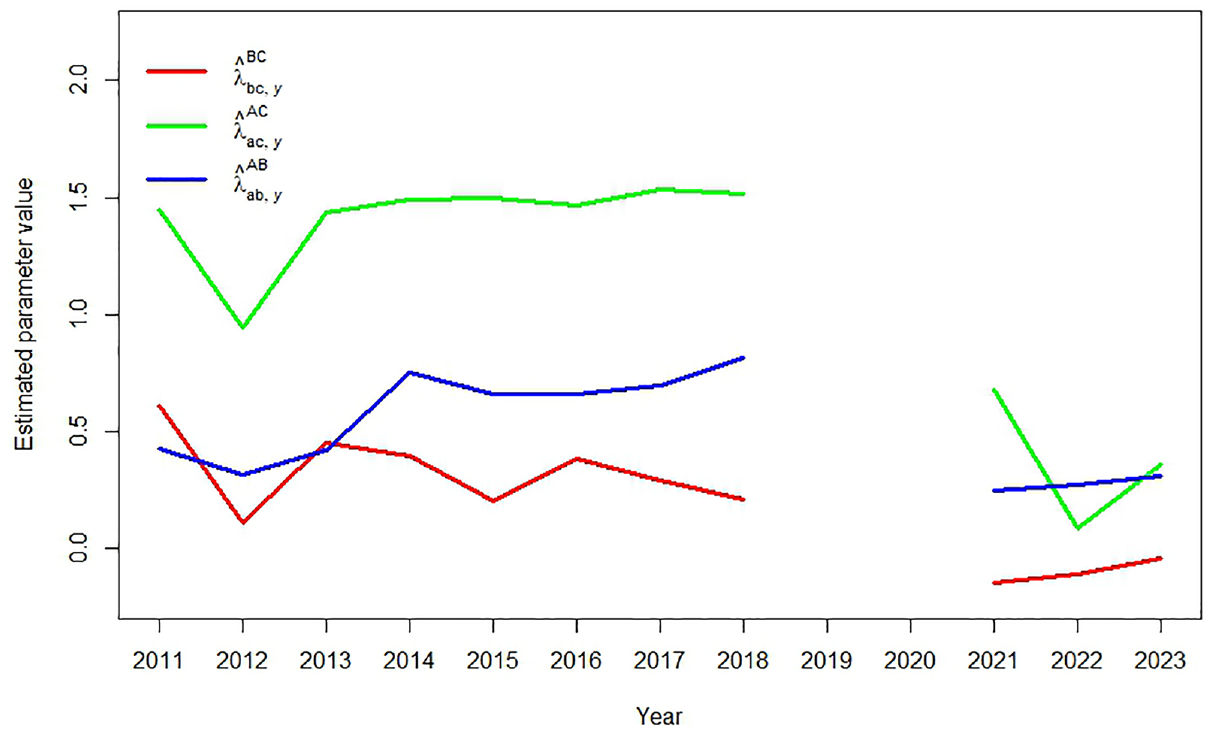
Both Figures 1 and 2 show that for some years and for some orders of sample availability the quality of the nowcast is better than for other years. Here it is interesting to note that both Figures indicate that the NC estimates are most accurate when sample $C_y$ is missing. This is somewhat surprising, because as Table 3 shows, sample $C_y$ is also the largest sample each year. An alternative reason for differences between NC and TSE estimates can be found in the stability of the pairwise-dependence parameter ${\lambda }_{\mathrm{ab},y}^{\mathrm{AB}}$ , as introduced in Equation (2), between two consecutive years. Note that this parameter can be estimated when the third sample for that year is available. Figure 3 below shows these estimates for ${\lambda }_{\mathrm{ab},y}^{\mathrm{AB}}$ , ${\lambda }_{\mathrm{ac},y}^{\mathrm{AC}}$ , and ${\lambda }_{\mathrm{bc},y}^{\mathrm{BC}}$ , over time.

Figure 3.

Coefficient estimates of ${\mu }_{\mathrm{ab},y}^{\mathrm{AB}}$ , ${\mu }_{\mathrm{ac},y}^{\mathrm{AC}}$ , and ${\mu }_{\mathrm{bc},y}^{\mathrm{BC}}$ over the periods $2011-2018$ and $2021-2023$ .

Figure 3 clearly shows three separate time series, which indicates that there is at least some stability in ${\lambda }_{\mathrm{ab},y}^{\mathrm{AB}}$ , ${\lambda }_{\mathrm{ac},y}^{\mathrm{AC}}$ , and ${\lambda }_{\mathrm{bc},y}^{\mathrm{BC}}$ over time. Figure 3 also shows that the estimated pairwise-dependencies became closer to zero when sample $B_y$ was replaced after $2019$ . This proximity to zero explains the larger accuracy of most of the DSE estimates in the years $2020-2023$ , as was shown in Figure 1. Ideally, each time series of estimates presented in Figure 3 are completely stable between periods. Long-term stability can in theory be tested with, for example, the well-known Dickey-Fuller unit root test (Dickey and Fuller 1979). However, this type of test requires the availability of a (much) longer time series to be reliable. A simple look at Figure 3 shows that stability between two consecutive years is not always the case, for example for ${\hat{\lambda }}_{\mathrm{bc},y}^{\mathrm{BC}}$ in $2012$ and $2013$ , and for in $2012$ , $2013$ , $2022$ , and $2023$ . We do not have an explanation for these shifts, but it is interesting to compare them to the time series in Figure 1 and the annual errors in Table 4. This comparisons shows that these larger shifts in ${\hat{\lambda }}_{\mathrm{bc},y}^{\mathrm{BC}}$ and ${\hat{\lambda }}_{\mathrm{ac},y}^{\mathrm{AC}}$ correspond to the years with larger nowcasting errors. This says that the stability of the pairwise-dependence parameter can be more important than the size of the missing sample.

5. Discussion

In this paper we propose to combine dual- and triple system estimation over two periods by means of the expectation-maximization algorithm to obtain a preliminary estimate, that we have coined an MSE nowcast estimate. The advantage of this approach is that, in the presence of older samples, it allows estimation with two (early available) samples, like in DSE. The difference with regular DSE is that the independence assumption in DSE can be replaced by a more relaxed assumption, that is, the pairwise-dependence of the two samples equals the corresponding pairwise-dependence in the previous period. Whether the NC estimates are accurate depends on the validity of this assumption.

Section 4 presents NC estimates on the number of homeless people in The Netherlands, which allowed us to evaluate the stability of pairwise dependencies of samples, for this example, in four different ways. First, the NC estimates were compared to the regular DSE estimates, which indicated that in our example for most years, the nowcast assumption of stable pairwise-dependencies is more realistic than the DSE assumption of pairwise-independence. Second, we checked whether the NC estimates were within the confidence intervals of the TSE estimates, which was mostly the case. Third, the NC estimates of $m_{001,y}$ were compared to the corresponding observations $n_{001,y}$ . Such a comparison is common in time series analysis, but rare in TSE, where population sizes usually remain unknown. This comparison showed that the estimates for $m_{001,y}$ and $n_{001,y}$ follow similar trends and are reasonably alike for most years, although for some years there are substantial differences. Finally, we estimated the pairwise-dependence parameters for the first two samples over time, which for each years becomes possible when the third sample is available. This analysis showed that for most years, the pairwise-dependence parameter estimates are reasonably stable, but not for each year. These unstable years directly correspond to larger differences between NC estimates and TSE estimates.

We conclude that our method to obtain NC estimates works and can be useful under two conditions. First, there needs to be some volatility in the population, because otherwise it may be easier and more accurate to simply use the population size estimate of the previous period. Second, the pairwise-dependence parameters of the first two samples needs to be reasonably stable. If this is not the case, the NC estimates can become seriously inaccurate, although they may still be more accurate than regular DSE estimates.

For future research, an alternative MSE nowcasting approach that is more closely related to traditional nowcasting models, is to combine a historic time series of MSE estimates with an historic series of MSE estimates that is based only on the smaller set of administrative sources that are available for the most recent period. For example, one may construct a historic time series of TSE estimates up till the previous period and construct a historic time series of DSE estimates, based on the same pair of samples, up till the current period, and combine both series in a, for example, (seasonal) autoregressive-integrated moving average ((S)ARIMA) model (Box 2013), with the DSE estimates as auxiliary series. The resulting model provides a TSE nowcast estimate for the current period that can be compared with the TSE nowcast estimate that results from the method suggested in this paper. However, such an approach would generally require longer time series than were available for the case discussed in this paper but may be an option in the future or in other cases.

References

1.
AlhoJ.1990. “Logistic Regression in Capture-Recapture Models.”Biometrics46 (3): 623–35. DOI: https://doi.org/10.2307/2532083.
2.
BaffourB.BrownJ.SmithP.2013. “An Investigation of Triple System Estimators in Censuses.”Statistical Journal of the IAOS29: 53–68. DOI: https://doi.org/10.3233/SJI-130760.
3.
BaffourB.BrownJ. J.SmithP. W.2021. “Latent Class Analysis for Estimating an Unknown Population Size – With Application to Censuses.”Journal of Official Statistics37 (3): 673–97. DOI: https://doi.org/10.2478/jos-2021-0030.
4.
BirdS. M.KingR.2018. “Multiple Systems Estimation (or Capture-Recapture Estimation) to Inform Public Policy.”Annual Review of Statistics and Its Application5: 95–118. DOI: https://doi.org/10.1146/annurev-statistics-031017-100641.
BoxG.2013. “Box and Jenkins: Time Series Analysis, Forecasting and Control.” In A Very British Affair: Six Britons and the Development of Time Series Analysis During the 20th Century. Palgrave Macmillan UK. DOI: https://doi.org/10.1057/9781137291264_6.
7.
BucklandS. T.GarthwaiteP. H.1991. “Quantifying Precision of Mark-Recapture Estimates Using the Bootstrap and Related Methods.”Biometrics47 (1): 255–68. http://www.jstor.org/stable/2532510 (accessed October15, 2024).
8.
CoumansM. A.CruyffM.van der HeijdenP. G. M.WolfJ.SchmeetsH.2017. “Estimating Homelessness in The Netherlands Using a Capture-Recapture Approach.”Social Indicators Research130 (1): 89–212. DOI: https://doi.org/10.1007/s11205-015-1171-7.
9.
DempsterA. P.LairdN. M.RubinD. B.1977. “Maximum Likelihood from Incomplete Data via the EM Algorithm.”Journal of the Royal Statistical Society: Series B (Methodological)39 (1): 1–38. http://www.jstor.org/stable/2984875 (accessed March21, 2024).
10.
DickeyD. A.FullerW. A.1979. “Distribution of the Estimators for Autoregressive Time Series with a Unit Root.”Journal of the American Statistical Association74 (366a): 427–31. DOI: https://doi.org/10.1080/01621459.1979.10482531.
EfronB.1979. “Bootstrap Methods: Another Look at the Jackknife.”The Annals of Statistics7 (1): 1–26. http://www.jstor.org/stable/2958830 (accessed October15, 2024).
13.
Equiza-GoñiJ.2022. “Real-Time Mortality Statistics During the Covid-19 Pandemic: A Proposal Based on Spanish Data, January–March, 2021.”Frontiers in Public Health10: 950469. DOI: https://doi.org/10.3389/fpubh.2022.950469.
14.
FienbergS. E.1972. “The Multiple Recapture Census for Closed Populations and Incomplete 2k Contingency Tables.”Biometrika59 (3): 591–603. DOI: https://doi.org/10.2307/2334810.
LincolnF. C.1930. Calculating Waterfowl Abundance on the Basis of Banding Returns. Vol. 118. United States Department of Agriculture. DOI: https://doi.org/10.5962/bhl.title.64010.
18.
LindsayB. G.1995. “Mixture Models: Theory, Geometry and Applications.”NSF-CBMS Regional Conference Series in Probability and Statistics5: i–iii+v–ix+1–163. http://www.jstor.org/stable/4153184.
StundzieneA.PilinkieneV.BruneckieneJ.GrybauskasA.LukauskasM.PekarskieneI.2024. “Future Directions in Nowcasting Economic Activity: A Systematic Literature Review.”Journal of Economic Surveys38 (4): 1199–233. DOI: https://doi.org/10.1111/joes.12579.
22.
Van den BrakelJ.MichielsJ.2021. “Nowcasting Register Labour Force Participation Rates in Municipal Districts Using Survey Data.”Journal of Official Statistics37 (4): 1009–45. DOI: https://doi.org/10.2478/jos-2021-0043.
23.
Van der HeijdenP. G. M.CruyffM.SmithP. A.BycroftC.GrahamP.Matheson-DunningN.2021. “Multiple System Estimation Using Covariates Having Missing Values and Measurement Error: Estimating the Size of the Māori Population in New Zealand.”Journal of the Royal Statistical Society: Series A (Statistics in Society)185 (1): 156–77. DOI: https://doi.org/10.1111/rssa.12731.
24.
Van der HeijdenP. G. M.WhittakerJ.CruyffM.BakkerB. F. M.van der VlietR.2012. “People Born in the Middle East but Residing in The Netherlands: Invariant Population Size Estimates and the Role of Active and Passive Covariates.”The Annals of Applied Statistics6 (3): 831–52. DOI: https://doi.org/10.1214/12-AOAS536.
25.
VanellaP.BaselliniU.LangeB.2021. “Assessing Excess Mortality in Times of Pandemics Based on Principal Component Analysis of Weekly Mortality Data-The Case of Covid-19.”Genus1 (77): 16. DOI: https://doi.org/10.1186/s41118-021-00123-9.
26.
WolterK. M.1986. “Some Coverage Error Models for Census Data.”Journal of the American Statistical Association81: 338–46. DOI: https://doi.org/10.2307/2289222.
27.
XuC.BainesP. D.WangJ.-L.2014. “Standard Error Estimation Using the EM Algorithm for the Joint Modeling of Survival and Longitudinal Data.”Biostatistics15 (4): 731–44. DOI: https://doi.org/10.1093/biostatistics/kxu015.
28.
ZultD. B.KriegS.SchoutenB.OuwehandP.van den BrakelJ.2023. “From Quarterly to Monthly Turnover Figures Using Nowcasting Methods.”Journal of Official Statistics39 (2): 253–73. DOI: https://doi.org/10.2478/jos-2023-0012.
29.
ZultD. B.van der HeijdenP. G. M.BakkerB. F. M.2023. “Bias Correction in Multiple-Systems Estimation.” arXiv Preprint arXiv:2311.01297. DOI: https://doi.org/10.48550/arXiv.2311.01297.
30.
ZwaneE. N.van der HeijdenP. G. M.2007. “Analysing Capture–Recapture Data When Some Variables of Heterogeneous Catchability Are Not Collected or Asked in All Registrations.”Statistics in Medicine26: 1069–89. DOI: https://doi.org/10.1002/sim.2577.
31.
ZwaneE. N.van der Pal-de BruinK.van der HeijdenP. G. M.2004. “The Multiple-Record Systems Estimator When Registrations Refer to Different but Overlapping Populations.”Statistics in Medicine23: 2267–81. DOI: https://doi.org/10.1002/sim.1818.