
Abstract
The International Passenger Survey (IPS) is undertaken by the Office for National Statistics to measure tourism flows and tourist expenditure, and international migration. It is interviewer-administered, and the questionnaire instrument was changed in 2017 to 2018 from a paper questionnaire (completed by the interviewer) to an electronic questionnaire administered with a tablet. For operational reasons no parallel run was possible, but the new questionnaire was rolled out progressively to sampling locations. This phased introduction supported the estimation of the effects of the new questionnaire on the main outputs from the survey. We describe initial simulations designed to estimate the power of the phased introduction approach to detect important difference in the IPS outputs, and analyses of the survey estimates at different stages up to the end of 2019 using state-space models, to estimate the discontinuities in the survey outputs. We make an assessment of the effectiveness of the overall approach.
1. Introduction
Border surveys are one strategy for gathering information on tourism and visits to a country (see Rideng and Christensen 2004, and Frenţ 2016 for summaries of border survey methodologies). The International Passenger Survey (IPS) is the United Kingdom (UK)’s border survey, and interviews people as they enter or leave the UK through ports, airports and the channel tunnel (the land border between Northern Ireland and Ireland is not covered). The sample design has two stages. In the first stage a stratified sample of time slots (from a population of morning and afternoon/evening slots at different airports/ports, covering 362 days of the year) is selected. Teams of interviewers work at the selected times and places, and there is a counting line, with interviews attempted with every kth traveler (for a suitable choice of k which may vary by stratum) crossing the line.
The IPS has been running since 1961, but the sample has been adjusted several times, most notably in 2009 when it was reallocated across a wider range of ports (ONS 2009). A detailed description of the history and methodology of the IPS is available in ONS (2014). The IPS has several purposes, including the measurement of tourism, the measurement of expenditures by visitors to the UK and by UK residents abroad, and the measurement of international migration. Migration filter shifts, designed to increase the number of migrants in the IPS sample, were introduced in 1980 to 1981. A very short questionnaire was used on these shifts, designed to identify migrants, who then received additional questions. Migration filter shifts were integrated with the main shifts in the 2009 redesign, but reintroduced in 2016 to increase the precision of migration estimates (White 2018). The IPS was suspended during the COVID-19 pandemic from March to December 2020, and has been replaced as a source of migration statistics by an approach based on administrative data and models (Rogers et al. 2021). A modified design was introduced in 2024. In this paper we focus on the changes to the IPS in 2017 to 2018, when migration was still a major topic of interest in the IPS.
The IPS interview is designed to be short and to be flexibly administered by interviewers to maximize response. Until 2017 data were collected on paper questionnaires (completed by the interviewer, except for some foreign language self-completion questionnaires (Pendry 2000)), and then mostly entered on-site using a laptop and a bespoke data capture tool programmed in Blaise (Statistics Netherlands 2002). The data could then be transmitted via a secure connection to a central database for further processing.
The ONS developed an electronic questionnaire for the IPS, to be administered using tablets. This was expected to have a range of benefits in the efficiency of the interviewers, and in the quality of the responses to the questions in the interview. We present these changes in more detail in Section 2 below.
Changing the data collection, and the associated changes in the questionnaire and editing procedures, had the potential to induce a discontinuity in the key IPS estimates for travel, tourism, and migration. Here a discontinuity is defined as a change in an estimate that results from a change in the collection approach and is not a change due to sampling variation or to a real evolution in the time series (Van den Brakel et al. 2008). Such a discontinuity needs to be measured, controlled, and understood in order that the IPS time series before and after the change can be compared accurately. For example, if collecting the data on tablets results in an increase in expenditure by overseas visitors, perhaps because responders can view the questions in their own language, the increase due to the change in the data collection needs to be measured. It is not a real change in expenditure and when comparing the series before and after the change an adjustment is needed to produce valid estimates of the real period-to-period changes of the variables of interest.
The recommended approach to dealing with possible discontinuities in time series resulting from changes to field procedures involves an embedded experiment in the survey, starting with a small experiment run with the new approach alongside the standard survey procedure. This is often referred to as a parallel run. If there is no evidence of a major change from this, then the sample with the new approach can be extended, and finally the new method is rolled out with only a small part retaining the original method (Van den Brakel et al. 2008, 2021). However, this kind of experimental design within an existing survey can be operationally challenging because of the need for interviewers to use different questionnaires and procedures simultaneously. The ONS therefore decided to make the change by a gradual roll-out to the various interviewing locations, which made the transition operationally feasible, because different interviewer teams operate in each location. This presents less information than a situation with an embedded experiment, where the treatments (different modes) can be randomized at some level, or a parallel run, but still provides a way to estimate the parameters of the transition with a state-space model. This kind of approach to analyzing transitions without a parallel run has been considered by Van den Brakel et al. (2020).
The purpose of this paper is to describe how a new field work strategy can be implemented in an ongoing survey in a situation where there is no capacity for parallel data collection. The new design is gradually phased in. To estimate the discontinuities in the key variables of the survey, a time series modeling approach is applied, where the effect of the redesign on the outcomes is modeled with a generalized version of a level intervention. This is achieved with an auxiliary variable that gradually changes from zero, for the period before the start of the implementation, to one, after complete implementation of the new design. During the transition period, the auxiliary variable reflects the proportion of the variables covered by the new design. A major drawback of this approach is that there is no control over the precision of the discontinuity estimates and that the initial estimates directly after the change-over are unstable. To manage this additional risk, a simulation prior to the start of the change-over is conducted to assess with what precision discontinuities can be observed and how many observations under the new survey design are required before stable estimates for the discontinuities are obtained. Additional risks, like confounding of the discontinuity estimates with unexpected events like Brexit, are discussed.
The paper is structured as follows. Section 2 summarizes the development of the tablet-based data collection, and the additional procedures and functionality that it offered. Section 3 describes the idealized measurement of discontinuities, and the constraints operating in the IPS field work which led to the roll-out. It sets out a state-space model for the evolution of the IPS series, and then uses the model in a simulation to assess the power of the rollout procedure to identify effects of given size. Section 4 describes the results of the implementation of the new questionnaire, and the estimated discontinuities as the time series developed. In Section 5 we discuss the findings and identify some lessons for the future.
2. Developing Tablet Data Collection for the IPS
The IPS has a number of different (but related) questionnaire instruments. There are arrivals and departures versions, relating to travelers entering or leaving the UK respectively, and trailers (additional survey instruments) for specific categories of travelers, including migrants, students, and employees. There are minor differences in the questionnaires to accommodate the different modes of travel (air, ferries, channel tunnel). For the purposes of the analyses in Sections 3 and 4 we assume that the mode of travel does not have an important effect separate from the direction of travel.
In order to move from paper to electronic capture, the questionnaire was redesigned to operate with the tablet screen (the early stages of this process are described in Benedikt (2015)). As part of this process the question wording and formatting was reviewed, to ensure it presented well on the screens. The routing was also considered; although the questionnaire is short, the different trailers make the routing quite complicated. One of the benefits of the change to an electronic questionnaire is that errors in routing were eliminated. The final design had one question per screen, and “there is evidence that respondents relate better to the ‘one-question-per-screen’ layout of the tablet, where they can see the questions in writing more easily themselves” (ONS 2018).
The new questionnaire allowed lookup tables for codes (e.g., for purpose of visit) to be automated; this was mainly a benefit for less experienced interviewers as experienced interviewers knew most codes automatically. The tablet questionnaire also implemented instant switching between languages in the display, based on the flag of the country as an indicator, which was much faster than the paper-based equivalent. This facilitated self-completion by travelers who did not speak English sufficiently well to undertake an interview. Some features could also be used to advantage, including the use of edit checks within the questionnaire (though many of these were treated as soft edits which could be overridden, in order to allow the interview to proceed quickly when necessary). The questionnaire could also be easily updated.
As a result of using the tablet questionnaire, a number of other changes to the survey process were also expected. The main changes include:
• the exercise of entering the data collected at the site would no longer be required. This process previously allowed for some quality assurance of the data close to the point of data collection;
• the post data collection editing (off-site by an editing team) was adjusted, because of the checks introduced in the questionnaire.
The new questionnaire was implemented in a limited pilot study before being included in the rollout. The pilot involved running several shifts at each of selected key survey sites over a two to three week period. This was sufficient to show qualitatively that the tablets were viable. The data collected suggested that the tablet questionnaire was better at capturing expenditure (largely because of the easier availability of questions in alternative languages in the tablet questionnaire), which would therefore be higher in the new mode.
There is a large body of literature on mode effects, see for example, Dillman and Christian (2005), de Leeuw (2005, 2008), Couper (2011), Dillman et al. (2014), and Schouten et al. (2022). Zhang et al. (2021) discuss and compare different onsite electronic survey data collection methods. Hassler et al. (2018) compared cost, completion times, and percent completion of electronic tablet to paper-based questionnaires administered onsite. Leisher (2014) compared tablet-based and paper-based survey data collection in terms of response rates, data collection costs, and completion time. Ravert et al. (2015) compared the equivalence of response obtained with paper based versus table-based questionnaires and reported only minor differences. Fanning and McAuley (2014) report non-significant effects between both modes in an experiment in a Health Survey questionnaire. Kusumoto et al. (2017) observed no difference in completion speed between paper and pencil and tablet surveys. Tourangeau et al. (2017) analyzed difference in measurement errors between surveys conducted on smartphones, tablets, and laptop devices. Although the results from these experiments cannot be generalized to the IPS we expect no large differences between the old and new approach, since both data collection approaches are based on interviewer administered data collection modes. Potential differences might be induced by the differences in the questionnaire.
Particularly in the context of mixed-mode surveys there is an increasing amount of literature on methods that attempt to correct and adjust for mode-effects. A regression modeling approach is proposed by Suzer-Gurtekin (2013). Imputation methods are proposed by Kolenikov and Kennedy (2014), while Vannieuwenhuyze (2014) and Klausch et al. (2017) propose adjustment methods based on re-interview designs. These methods focus on equalizing mode effects in mixed-mode designs and are not directly applicable in a change-over from one uni-mode design to another uni-mode design where the questionnaire changed simultaneously.
3. Planning for and Dealing with Changes in Survey Procedures
3.1. Randomization or Deterministic Transition
The best conditions for the estimation of a discontinuity are to use an embedded experiment with the new and old approaches as the treatments (Van den Brakel et al. 2021). This effectively gives a parallel run of the new and old methods, and allows the independent estimation of the discontinuity and the real evolution of the time series. There are several levels at which randomization of treatments could be undertaken in the IPS. These levels and the expected sample sizes from a 10% treatment group are:
(a) by interview, n ≈ 2,500
(b) by interviewer shifts, n ≈ 100
(c) by interviewers and flows (arrivals/departures), n ≈ 40
(d) by interviewers, n ≈ 20
(e) by site, n ≈ 5.
The effective sample size for (b) to (e) would however be reduced by the clustering of observations within the experimental units, and therefore the power of these designs to detect a difference would generally be low. ONS’s assessment of the operational considerations in introducing the changes to the IPS was that the randomization of cases, interviewers, or shifts would introduce too much disruption to the fieldwork and therefore risk the quality of the outputs. There was also a requirement to progressively roll-out training for interviewers that made a staged transition team by team (where a team of interviewers may cover a single site or a group of sites) the most practical implementation approach. The inflow and outflow questionnaires have some differences, so interview teams were trained first on the new outflow questionnaire, which was implemented first, then later on the inflow questionnaire. Therefore the rollout patterns are different on the two sets of variables. This meant that a parallel collection on both methods would not be available, and methods based on the availability of parallel run data (e.g., Van den Brakel et al. 2021) were effectively ruled out.
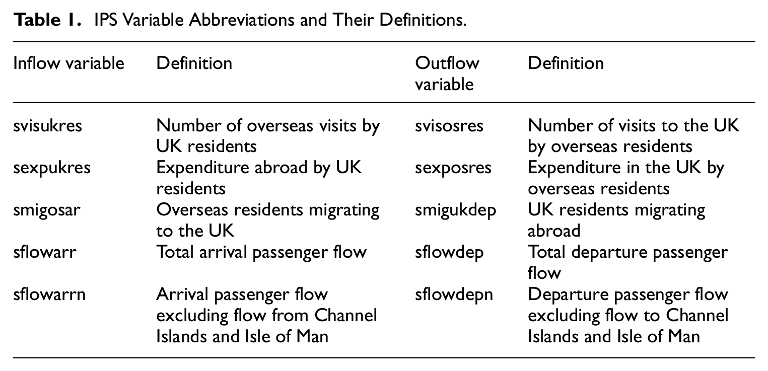
Without a parallel run the estimate of the discontinuity is confounded with the normal evolution of the time series, but by making assumptions about that evolution, the discontinuity can be estimated (Van den Brakel et al. 2008, 2020). The staged transition across IPS sites gives an increasing coverage of the main IPS variables by the tablet questionnaire (the variable abbreviations used here and their definitions are given in Table 1). The proportion of each variable which is moved to tablet data collection at each stage of the process is shown in Table 2; these are different for different variables because the characteristics of passengers vary by airport.
IPS Variable Abbreviations and Their Definitions.
Estimated Proportions of IPS Variables Covered by the Staged Transition to the Tablet Questionnaire.
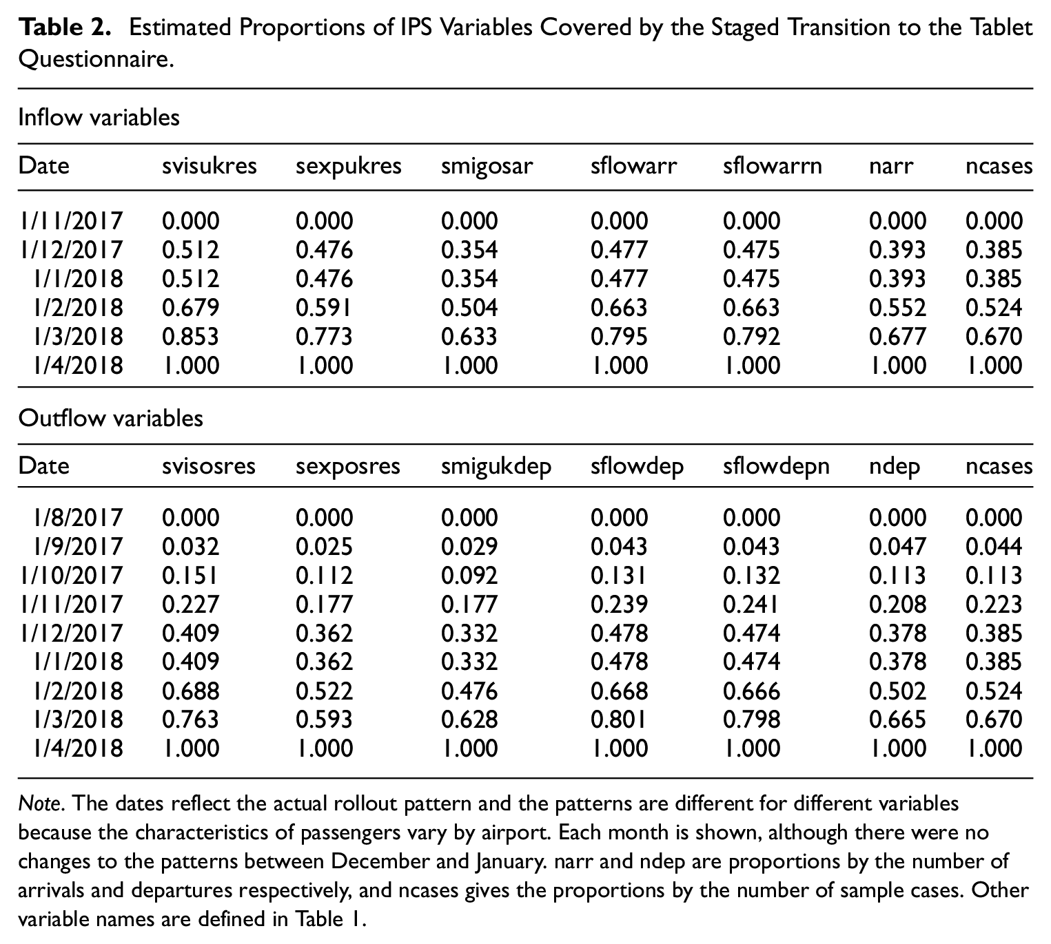
Note. The dates reflect the actual rollout pattern and the patterns are different for different variables because the characteristics of passengers vary by airport. Each month is shown, although there were no changes to the patterns between December and January. narr and ndep are proportions by the number of arrivals and departures respectively, and ncases gives the proportions by the number of sample cases. Other variable names are defined in Table 1.
Before the change to the tablet questionnaire was implemented, an indication of the power of the analysis to detect a discontinuity in the different series was required, as part of the communication with users about the expected effects of the transition. The power can be assessed by simulation using a suitable model for the evolution of the monthly IPS estimates (Van den Brakel et al. 2020). So we first present a model for the IPS variables in Subsection 3.2, then return to the assessment of power in Subsection 3.3.
3.2. The Model
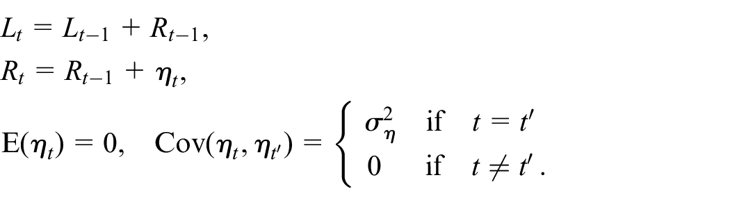
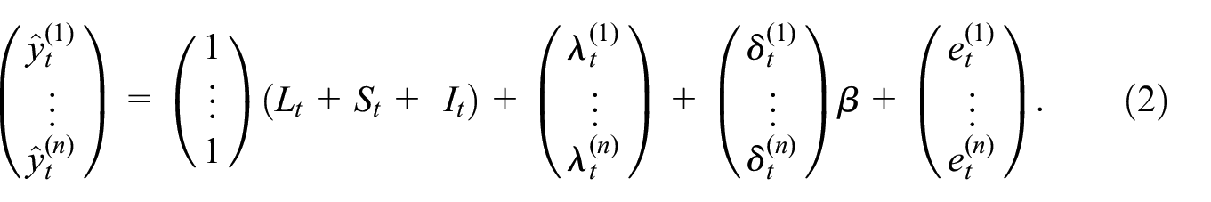
The monthly estimates of the IPS output variables were used to develop a structural time series model. The model used to represent the evolution of the IPS series yt is

where
Note that the level of the trend can implicitly contain a deterministic level, that is,
with
and
Finally, xt represents an indicator explanatory variable which takes the value 0 before the discontinuity is introduced, then an increasing positive value (as in Table 2) as the rollout progresses, and then the value 1 once rollout is completed and for all subsequent periods. It can be interpreted as a generalized version of a level intervention variable. The fitted parameter
For the trend, the so-called smooth trend model is chosen. This is a popular trend model in econometric time series modeling (Durbin and Koopman 2012, Ch.3). See Subsection 3.4 for a more extended motivation and a comparison with the local level trend model. Also the trigonometric seasonal is a standard model in econometric time series modeling (Durbin and Koopman 2012, Ch.3) and is an appropriate specification to model a seasonal pattern as visible in Figure 1. The level intervention approach to estimate the effect of an intervention was originally proposed by Harvey and Durbin (1986) to estimate the effect of seatbelt legislation on road causalities. Van den Brakel et al. (2008, 2020, 2022) and Van den Brakel & Roels (2010) used this approach to estimate discontinuities in repeated sample surveys induced by a redesign of the survey process. A recent similar application is for example, Hungnes et al. (2024).
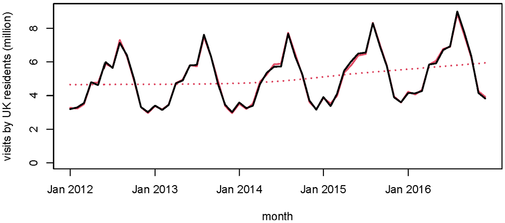
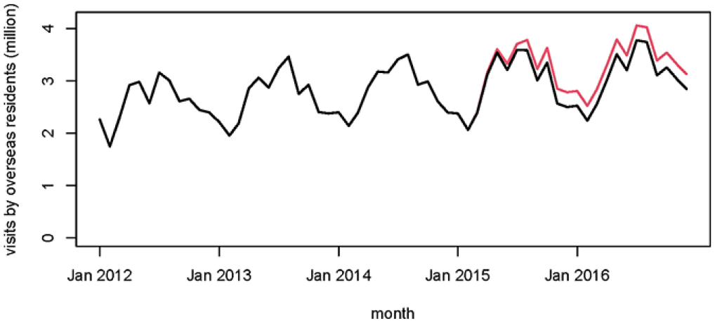
Original series of estimates of visits abroad by UK residents svisukres (black), the Kalman smoother estimates of the signal from the state-space model (solid red), and the trend from the model (dotted red).
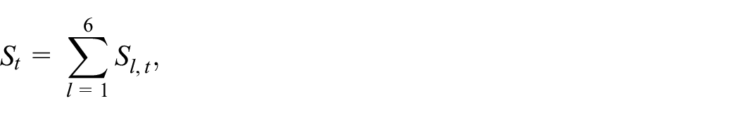
An alternative approach is to construct time series for each airport separately, combine them in one multivariate model and model the effect of the transition in each series with a level intervention. Let
Here

The
To avoid the rescaling of the input series to the national level, a Seemingly Unrelated Time Series Equation (SUTSE) model can be considered. In this case
The models are expressed in state-space form, and the Kalman filter is used to estimate the state variables (Durbin and Koopman 2012). The state space representation distinguishes between state variables and hyperparameters. The state variables define the trend (
The Kalman filter is a recursive algorithm that starts at the beginning of the series and provides for each period t optimal estimates and standard errors for the state variables based on the time series observed until period t. These are referred to as the Kalman filter estimates. The Kalman filter estimates for each period t, can be updated with the information that became available after period t. This procedure is called smoothing and is based on a recursive algorithm that starts with the last observation of the observed series and updates the filtered estimates, including their standard errors, for the state variables of all preceding periods. These are referred to as the Kalman smoother estimates. Under the assumption that the disturbance terms and the initial state vector are normally distributed, the Kalman filter provides optimal estimates in the sense that they minimize the mean squared error. If the normality assumption doesn’t hold, the Kalman filter is still an optimal estimator in the sense that it minimizes the mean squared error within the class of all linear estimators (Harvey 1989, Subsection 3.2). The stated normality assumption implies that the one-step-ahead prediction errors are normally and independently distributed. This is evaluated by testing the standardized one-step-ahead prediction errors for (1) heteroscedasticity using an F-test, (2) normality using a Bowman-Shenton test, and (3) autocorrelation using a Ljung-Box test (Durbin and Koopman 2012, Subsection 2.12).
To start the Kalman filter, initial values for the state variables as well as values for the hyperparameters are required. Equation (1) contains non-stationary state variables, which are initialized with a diffuse initialization. This implies that the initial values of all state variables are equal to zero with a diagonal covariance matrix with diagonal elements diverging to
The values of the hyperparameters are also unknown. They are estimated by means of maximum likelihood. The likelihood function is obtained by the so-called prediction-error decomposition (Harvey 1989, Subsection 3.4). The likelihood function is optimized by repeatedly running the Kalman filter in a numerical optimization procedure using MaxBFGS (Doornik 2009). Since the hyperparameters are variances, which cannot take negative values, they are estimated on the log-scale. The starting values for the hyperparameters in the optimization procedure are equal to
We expected that the IPS, which is not designed to produce estimates for single months for most variables would be rather volatile, but the models were surprisingly well-behaved. Figure 1 shows an example from the modeling of the number of trips by UK residents, measured on the passenger inflow, svisukres. The black line shows the original data, and the red solid line the Kalman smoother estimates for the trend and seasonal of the model, Equation (1), with
3.3. Power Assessment
The basic strategy then is to take a period of the IPS equal in length to the proposed rollout, to assume a level of discontinuity (consistently across sites within a flow), and to introduce this discontinuity to the series according to the pattern of the rollout. This creates an adjusted series which is used as the input to a model which includes the rollout pattern xt, and an estimate is made of the size of the discontinuity and its variance. We expect early estimates to be far from the truth (as early in rollout few ports will be using the tablet questionnaire and there is little information on which to base an estimate of the discontinuity), but to converge to a more stable estimate as further information on the size of estimates with the tablet collection accumulates. Even beyond the rollout period, additional information about the size of the discontinuity is obtained as the parameters of the model are affected by new observations. This allows us to assess the size of discontinuity which is likely to be detectable (i.e., the power of such an analysis) and the time required to obtain a stable estimate for the discontinuity.
We examine one variable, the number of visits by overseas residents, svisosres (which is measured on the outflow), in detail to demonstrate the approach that has been followed.
The first step is to introduce a discontinuity (as a percentage of the mean of the series from January 2012 until December 2016) into the existing series. Figure 2 shows the original series and the discontinuity, which is phased in over eight months in accordance with the rollout plan on the outflow. We show the actual periods of the data on the x axis, though the real time periods are not important for this simulation. The new (red) series from Figure 2 now contains the discontinuity, but also the sampling error from the IPS in the periods used, which is expected to obscure the discontinuity. Equation (1) is fitted to this new series, now with
Original (old) series of estimates of the number of visits to the UK by overseas residents svisosres (black), and the new series (red) after a 10% discontinuity has been phased in over eight months from March 2015.
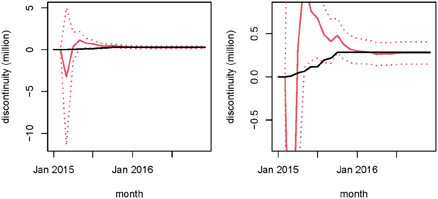
In black the “real” discontinuity in the series during and after completion of the phase-in period (i.e.,
The first thirty-six months of the series are not shown in Figure 3, as no discontinuity is expected by the model so nothing happens—although this period does allow the parameters of the other components of the Kalman filter to stabilize from their starting values. The initial erratic behavior of the discontinuity estimate is clearly seen, and some of the early estimates of the discontinuity do not contain the “real” series within the confidence interval. By the time the rollout is completed in October 2015 (the eighth month of the rollout) the estimate is much improved and the confidence interval much narrower (although in this particular example the “real” change is only just in the interval at this stage). Around January 2016 the estimate has essentially converged on the correct value, although the confidence interval continues to get slightly smaller until September 2016.
This example shows the situation with a discontinuity of a particular size in a particular month. The same discontinuity appearing at a different point in the evolution of the series may have a different impact on the results, so in another experiment the same rollout pattern is applied starting from September 2014. This produces qualitatively the same pattern, although there are some differences of detail. In this case the estimated discontinuity does not stabilize until around July 2015 (the eleventh month after the rollout). We also used the same procedures with a −5% discontinuity, again introduced at two separate time points. Table 3 summarizes the effects of these procedures in these four example cases.
Summary Statistics for Example Discontinuities of +10% and −5% Applied to the IPS svisosres Series at Two Different Times.
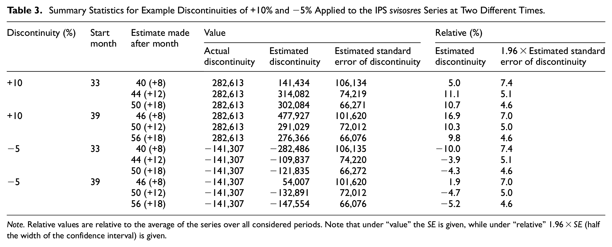
Note. Relative values are relative to the average of the series over all considered periods. Note that under “value” the SE is given, while under “relative” 1.96 × SE (half the width of the confidence interval) is given.
The evolution of the estimated standard errors are almost the same regardless of the size of the discontinuity or the month in which it is introduced. So for this variable we expect to have the power to detect a change of approx. 200,000 at the end of the roll-out; 150,000 four months after the end of roll-out; and 130,000 ten months after the end of roll-out, as follows from the standard errors reported in Table 3. This is just enough in this case to detect a 5% change.
The example of svisosres works quite well, but this is not always the case. Figure 4 shows sflowarrn with a +5% discontinuity. Here the estimated discontinuity does not converge toward the real (induced) one, but instead to a lower value which eventually leaves the true discontinuity more or less outside the confidence interval.
In black the “real” discontinuity in the series during and after completion of the phase-in period (i.e.,
Table 4 gives an overall summary of the approximate minimum detectable effects at the end of roll-out, end of roll-out + four months, and end of roll-out +ten months for variables on both flows, based on the estimated standard errors from the simulations.
Approximate Minimum Detectable Effects (Rounded to the Nearest ½% Below 10, or Nearest 1% Above It) for Analyzed Variables, at the End of the Roll-Out Period, and Four and Ten Months After It.
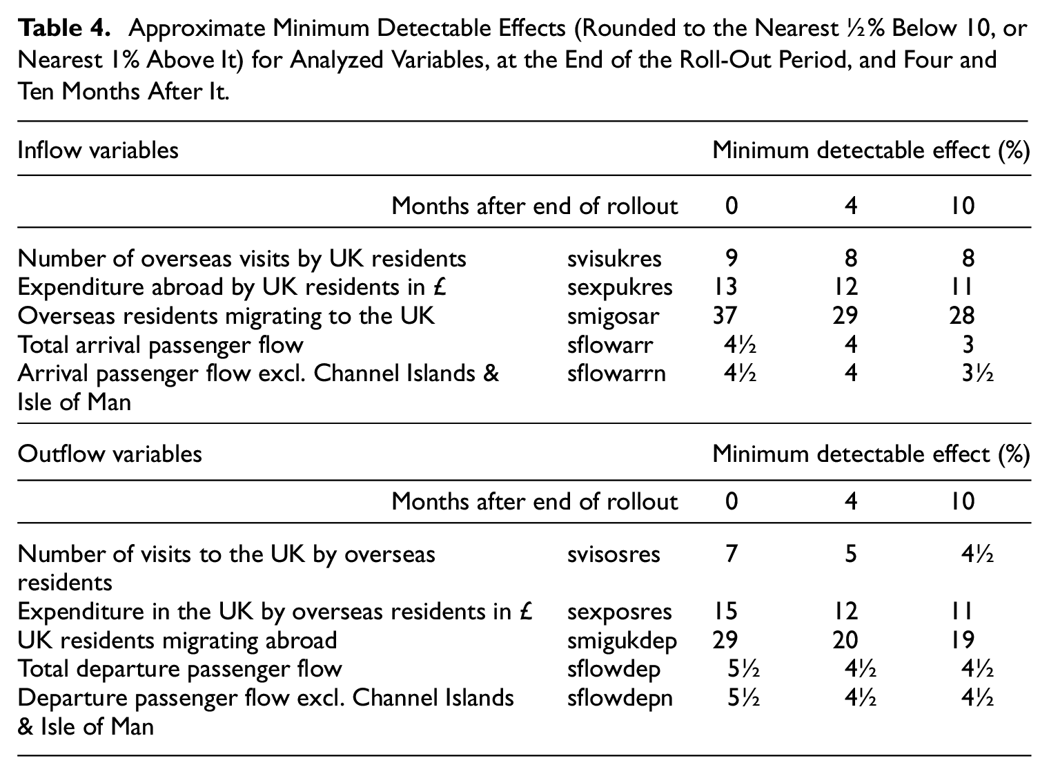
It can be seen that only the largest discontinuities in the migrant flows are expected to be detectable, and that expenditure differences less than 10% are not expected to be detectable. But on other person-based flows discontinuities of around 5% will generally be detectable.
3.4. Simulation with Different Trend Models
In this subsection the choice for a smooth trend model is motivated for
A statistical argument for a choice between the smooth trend model and the local level model is the order of integration of the observed series. The smooth trend model assumes a second order of integration, I(2), for the observed series while the local level model assumes a first order of integration, that is, I(1). An Augmented Dickey-Fuller (ADF) test rejected the null hypothesis for all series that there is a second order unit root (all p-values smaller than 1%). This would motivate the choice for a local level model instead of a smooth trend model.
Applying a local level model to the IPS series results in more volatile trend estimates compared to the smooth trend model. This affects the estimates for the discontinuities. The smoother the trend the greater the influence of observations that are further away from the time of transition on the discontinuity estimates. With the local level trend model, more weight is given to the observations directly before and after the transition. With the smooth trend model observations further away from the transition also contribute to the discontinuity estimates.
Since the results for the discontinuity estimate depend on the choice for the trend model, a simulation was conducted. The setup is similar to the simulation discussed in Subsection 3.3. For the series observed between January 2012 and December 2016, a discontinuity of 10% of the level of the series in 2016 is added to the series, proportional to the roll-out in Table 2, assuming that the roll-out starts in January 2014. In a next step, the discontinuities are estimated with the model in Equation (1), once with a smooth trend model for
Simulation Results for Discontinuity Estimates with a Smooth Trend Model and Local Level Trend Model.
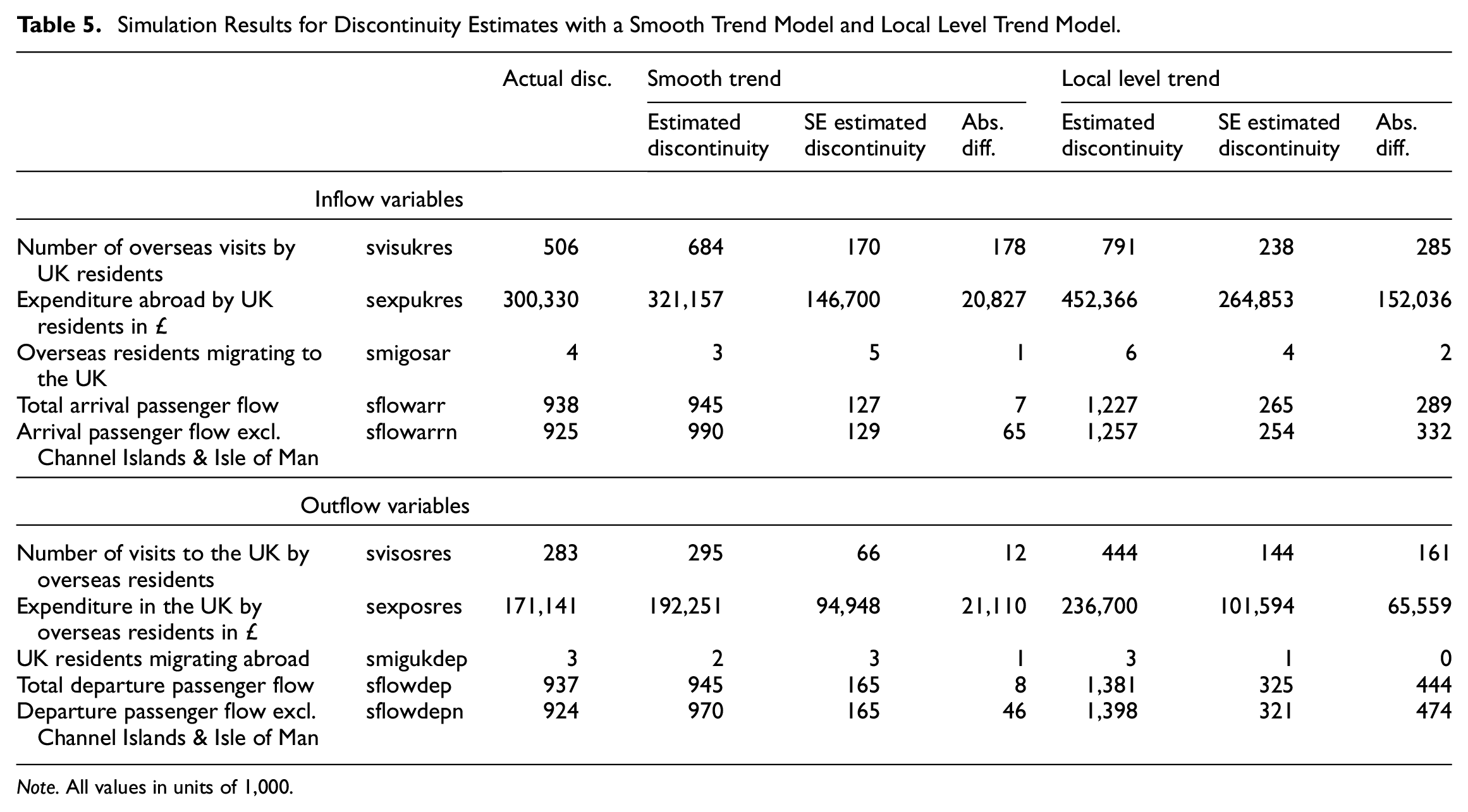
Note. All values in units of 1,000.
Finally the model assumptions of both state space models are tested by evaluating to what extent the one-step-ahead prediction errors meet the assumption that they are normally and independently distributed. To this end the following tests (see Durbin and Koopman 2012, Subsection 2.12 for an overview) are applied to the standardized innovations: (1) F-test for heteroscedasticity, (2) Bowman-Shenton test for normality (Bowman and Shenton 1975), and (3) Ljung-Box test (Ljung and Box 1978) for serial auto correlation up to lag 12. Results are included in Appendix B and indicate some deviation from the normality assumption for about half of the series. Based on these model diagnostics, however, there is no preference for one of the two trend models.
Based on these considerations the smooth trend model is used in Equation (1). Even though the ADF test clearly rejects the null hypothesis that the series contain a second order unit root, the simulation clearly indicates that the smooth trend model is more appropriate for estimating discontinuities. In addition the Ljung-Box test statistics in Tables B1 to B3, provide comprehensive evidence that the chosen smooth trend model is adequate. If the data were I(1) and the smooth trend model was misspecified, the one-step-ahead prediction errors should be over-differenced and thus autocorrelated. This is, however, ruled out by the test results of the Ljung-Box test for almost all series. An interesting interpretation, proposed by a constructive reviewer, is that the structural break overshadows the persistent characteristics of the series. If for example, the break has a strong signal whereas the I(2) trend is comparably smooth, then the ADF test may reject even in the presence of an I(2) trend. This could be tested with an ADF test that is robust to structural breaks, for example, with a slightly modified version of the GLS-type ADF test by Elliott et al. (1996). Since the simulation results and diagnostic tests are already convincing, this is left for further research.
The maximum likelihood estimates for the hyperparameters, with their standard errors for the finally selected model are included in Appendix C.
4. Evaluation of Discontinuities
There was a natural desire to make an assessment of the discontinuity as quickly as possible after the tablet questionnaire was in use, in order to inform users about the impacts of the change on the time series of estimates. The published estimates were accompanied by warnings that the quality of estimates of change would be reduced during and after the rollout of the new questionnaire, but there was pressure from users of the statistical outputs for more certainty in how the estimates could be used. The evidence from Table 4 is that the longer the elapsed period after the rollout, the better the estimation of the discontinuity becomes (though with reducing benefits of additional months).
This led to several assessments of the size and importance of the discontinuities on the main IPS output variables during the period after the rollout. We give some examples of each of these below, starting with an assessment after two months in Subsection 4.1. The analysis periods were only chosen after the rollout, so did not correspond exactly with those chosen in the power analysis.
Recall from Section 3 that without a parallel run, the estimation of the discontinuity relies on some assumptions about the stable evolution of the underlying time series of estimates. The period of rollout was however affected by changes to traveler and migrant behavior driven by the period of uncertainty over Brexit. The Brexit referendum was in June 2016, but the two-year transition period was coming to an end just after the rollout, so there was an unusual amount of migration and some changes to tourism in expectation. So a priori we might expect that the model will not be as effective, since the actual changes are affected by Brexit, and these might obscure the effect of the discontinuity. We return to this topic in Section 5.
Since some of the key IPS variables are monetary and many of the values being estimated are large, we also considered that the variance could increase with the estimate, which would suggest that a log transformation would be needed to stabilize the variance. We therefore applied the same models to log-transformed data, though in most of the variables analyzed this did not provide a substantial improvement.
4.1. Early Estimation of Discontinuities
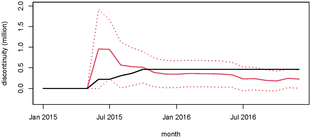
An initial analysis used data up to June 2018, which covered the roll-out period (September 2017–April 2018) and (since the roll-out was essentially completed by early April) three months afterward. The minimum detectable effects would be expected to be between the zero- and four-month columns in Table 4 if the series behaved as in the test data. Figure 5 (left) shows the estimated discontinuity for svisosres. In this case the estimate seems to be close to stabilizing, although it is hard to say what will happen when additional data points are added. The estimated discontinuity (in millions of people) in June 2018 is −0.244 ± 0.153—significantly different from zero, but not very accurately estimated. This discontinuity is around 7% (% discontinuity values are calculated relative to the estimate of the trend at the given time throughout. They are therefore not affected by seasonal variations), which is around the smallest detectable difference according to the earlier power analysis. This was the only variable where the estimated discontinuity was significantly different from zero at this stage.
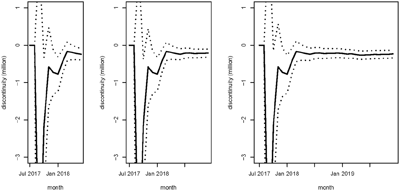
Estimated discontinuity (millions of visits) and its 95% confidence interval for the number of visits to the UK by overseas residents svisosres; (left) based on data up to June 2018; (center) based on data up to December 2018; (right) based on data up to December 2019. Periods before the rollout begins have estimated discontinuity of zero and are not shown before July 2017.
By contrast, Figure 6 shows the estimated discontinuity for sexpukres, and here there is no sign that the estimate has stabilized yet. The latest month’s estimate is still quite different from the previous month, and the estimated confidence intervals are wide. The discontinuity is around 3%, considerably smaller than the minimum detectable difference from the power analysis. The apparent lack of stabilization may therefore result only from the inability of the model to detect a discontinuity of this size with the current design.
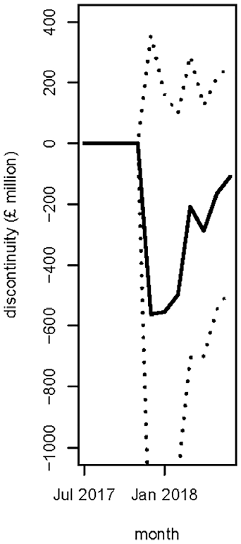
Estimated discontinuity (£m) and its 95% confidence interval for expenditure abroad by UK residents sexpukres, based on data up to June 2018.
In both of these examples, the behavior of the trend component of the models has not changed as a result of the addition of the latest data. This suggests that there has been no detectable effect of Brexit, or possibly that some of the Brexit effect has been picked up in the estimate of the discontinuity.
Across all the variables considered, most of the estimates of discontinuities are not significantly different from zero at this stage, and are smaller than the anticipated minimum detectable effects from Table 4. Nevertheless, some of the estimated discontinuities are large, up to 20%, and the effects on (for example) the estimated numbers of migrants would be relevant to users.
Almost all of the discontinuity estimate are negative, which means that the measurement made with tablets is lower than the previous paper-based measurement. This seems to contradict the initial indications from the pilot study, which were that the tablets were better at capturing expenditure, which was therefore higher in the new mode. The pilot used a small sample, however, and results from it may not be a strong indicator of direction of the discontinuity. If the indications of direction of the discontinuity from the pilot were correct, it is possible that the size of the discontinuity is at least in part confounded with changes in migration and expenditure patterns influenced by changing exchange rates and uncertainty over Brexit.
4.2. Estimation as the Basis for Deciding on an Adjustment
The second assessment used data up to December 2018, covering the roll-out and eight months afterward. This was the main “live” evaluation to make a judgment about whether to make a formal adjustment to the IPS estimates, since it was felt that users could not wait longer for an official assessment. The minimum detectable effects would be expected to be close to the 10-month columns in Table 4 if the series behaved in the same way as in the test data.
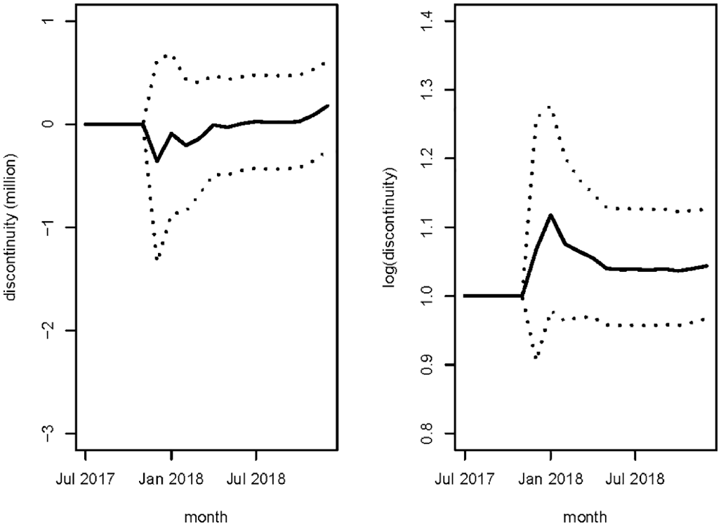
In Figure 5 (left panel) we subjectively assessed that the estimated discontinuity for svisosres was close to stabilizing. With the additional data to December 2018 we can see the evolution of this series (Figure 5, center panel).
The estimated discontinuity (in millions of people) estimated with data up to December 2018 is −0.212 ± 0.107, slightly smaller than the discontinuity estimated using the earlier data only, and with the variance halved. The estimated discontinuity for this variable is significantly different from zero, and the discontinuity is around 6%, which is larger than the smallest detectable difference at this stage according to the earlier power analysis (Table 2).
Most of the series had estimated discontinuities which had stabilized over the period considered. Svisukres shows different behavior however (Figure 7, left panel).
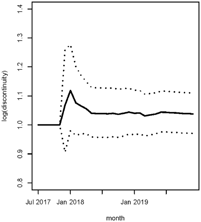
Estimated discontinuity (millions of visits) and its 95% confidence interval for the number of overseas visits by UK residents svisukres (left) and log(svisukres) (right), based on data up to December 2018.
This clearly has not stabilized, and the estimated discontinuity has a wide confidence interval. We tried the log transformation for this variable, and estimated the discontinuity in the transformed variable. This gives us the filtered estimates in Figure 7 (right panel), which have stabilized, an instance where the log transformation is clearly helpful. The log transformation implies a multiplicative model. The fitted parameter can be interpreted as a proportional discontinuity in the series. The power was not assessed on the log-transformed data, so we cannot see whether the effects are in the range that was expected to be identifiable.
In all the series considered using data up to December 2018, the behavior of the trend components of the models continues to be unchanged. This suggests that either there has been no detectable effect of Brexit on the trend, or possibly that some of the Brexit effect has been picked up in the estimate of the discontinuity. It is not possible to disentangle these alternative explanations further with the collected data.
Only two of the estimated discontinuities are significantly different from zero (svisosres and sexposres), and only these two estimates are larger than the anticipated minimum detectable effects in Table 4. Where the estimated discontinuity is not detectable (note that this is not the same as saying that no discontinuity is present, just that we have not been able to detect it with the statistical power of the fitted model), making an adjustment would involve an assumption about the stability or evolution of the discontinuity estimate outside the period of the analysis. Combined with the uncertainty in estimating the discontinuity, an adjustment would therefore not improve the quality of the series of estimates.
The two series with estimated discontinuities significantly different from zero are more problematic. First, we actually make assessments for ten variables (though two pairs of variables are so similar (Table 1) that there are probably only eight independent tests). A Bonferroni type correction to the significance level would mean that neither discontinuity would continue to be significant. Second, we are concerned that some of the actual evolution in the series due to behavior changes induced by the approaching Brexit deadline have been incorporated in the estimated discontinuity. For these two reasons it was decided that no adjustment was warranted in these two series either.
4.3. Retrospective Evaluation
It was also possible to revisit the series up to December 2019, including the rollout and a further twenty months. This is in fact almost the longest period that can be available for evaluation, since the IPS series were strongly disrupted from late March 2020 by the COVID-19 pandemic. Any adjustment to the state-space model from Subsection 3.2 to make the trend sufficiently responsive to include this period would automatically mean that the trend at the time of the discontinuity was not affected by the new data, so nothing would be gained from adding anything further.
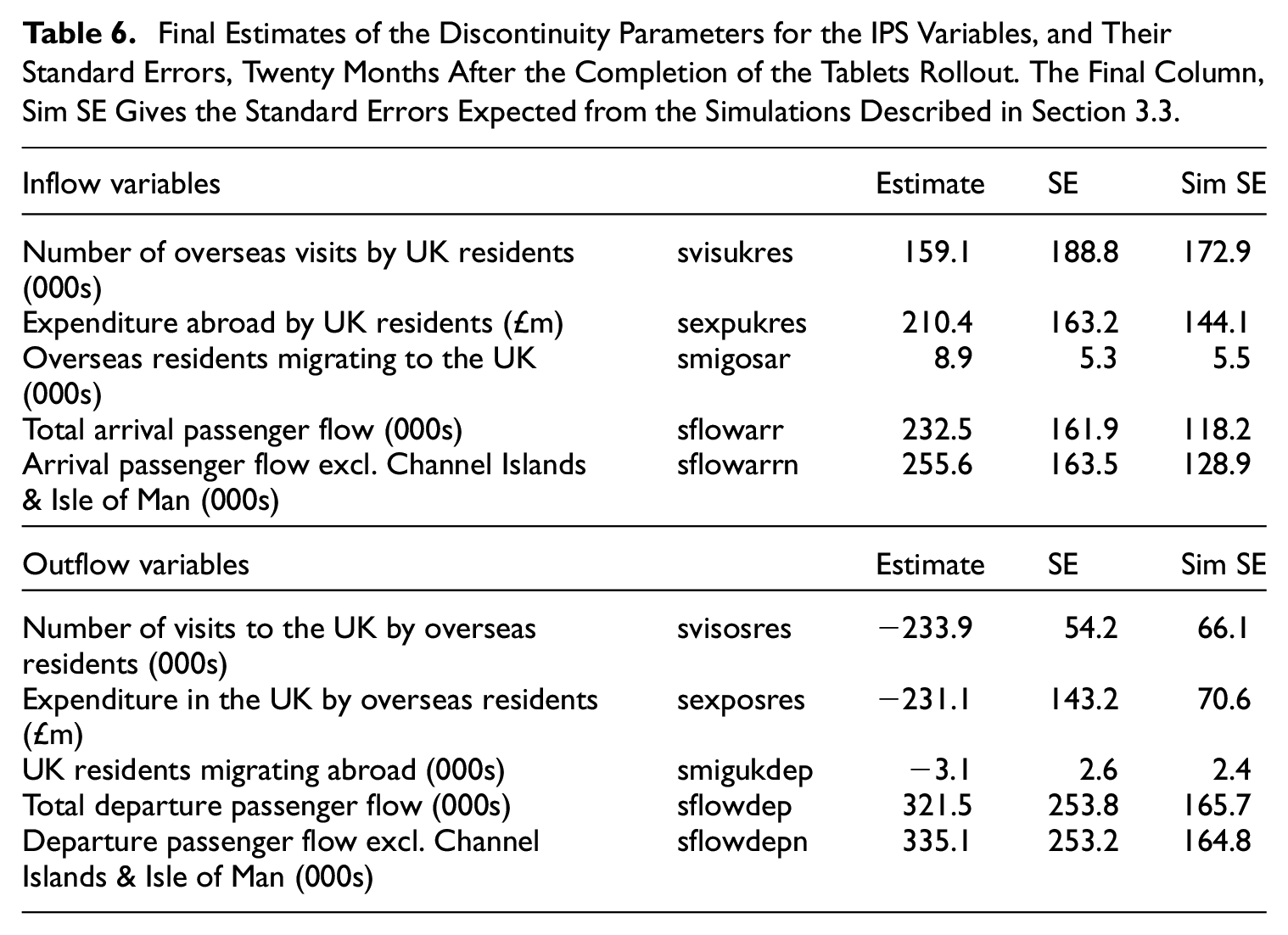
The extra year of data makes almost no difference to the conclusions drawn at the time a decision on adjustment was made. Two of the estimated discontinuities are significantly different from zero, and svisukres continues to be the only series where the log transformation leads to a substantial improvement in the stability. The evolution of the discontinuity estimates is shown for svisosres and log(svisukres) in Figures 5 (right panel) and 8 respectively.
Estimated discontinuity and its 95% confidence interval for the log of the number of overseas visits by UK residents, log(svisukres), using data up to December 2019.
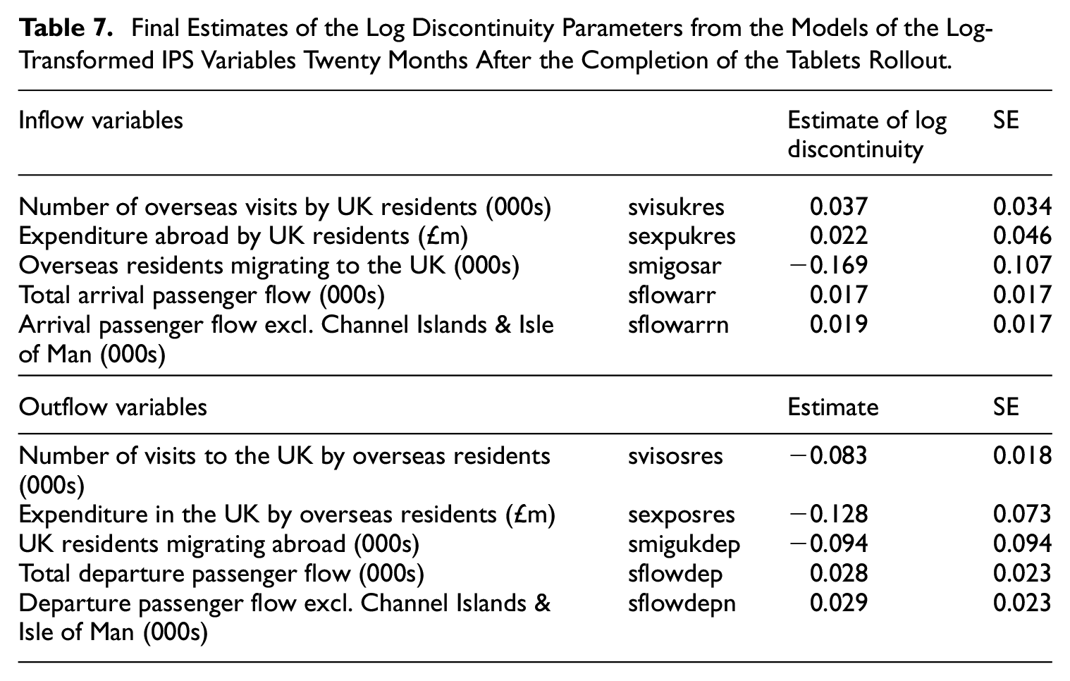
Table 6 shows the estimated effect of the change to tablet data collection in the IPS for all the considered variables and their standard errors. Only svisosres has a discontinuity which is significantly different from zero, and this is also the only variable where the estimated discontinuity is close to the minimum detectable effect from Table 4.
Final Estimates of the Discontinuity Parameters for the IPS Variables, and Their Standard Errors, Twenty Months After the Completion of the Tablets Rollout. The Final Column, Sim SE Gives the Standard Errors Expected from the Simulations Described in Section 3.3.
We did not further extend the time series with the observations that became available after December 2019. As a result of the COVID 19 crisis, international passenger traffic virtually ground to a halt, resulting in a huge disruption of the time series and a sudden misspecification of the model in Equation (1). There are several ways to account for these shocks in the model, Equation (1). One approach is to increase the flexibility of the trend component by making the variance of the slope disturbance terms time varying, see Van den Brakel et al. (2022) for details. In addition a major adjustment of the seasonal component would be necessary. The consequence of such interventions is that data observed after the start of the corona crisis do not add additional information to the estimate of the discontinuities. On top of that it was already established that the series observed until December 2019 provided enough information to obtain stable estimates for the discontinuities.
In Subsection 4.2 we saw that log transformation of the data was potentially useful for one variable. We therefore examined the performance of the models with log transformations for all the variables in the transition, and the results of these are presented in Table 7. With the log transformation the models meet the normality assumption of the state space model better (see Appendix B, Table B3); nevertheless we prefer the models on the original scale as the interpretation of the discontinuity is more straightforward.
Final Estimates of the Log Discontinuity Parameters from the Models of the Log-Transformed IPS Variables Twenty Months After the Completion of the Tablets Rollout.
5. Discussion
The changes to the IPS field procedures could only be managed with a phased transition from the old to the new tablet-based questionnaire, which did not allow for a randomization of the two questionnaires as treatments in an embedded experiment. A drawback of the time series modeling approach is that there is no control over the precision and the size of the discontinuities that can be observed, which increases the risk that substantial discontinuities cannot be assessed. To assess the size of the discontinuities that can be detected with a time series modeling approach before the start of the transition to a new survey design, a simulation is proposed. If such a simulation indicates that the time series modeling approach is insufficient to detect discontinuities that are of importance of the data users, then the precision can be improved by combining the time series modeling approach with a (small) parallel run. The direct estimates for the discontinuities and their standard errors obtained with the parallel run can be used in the time series model through an exact initialization of the Kalman filter. The data observed before and after the change over to the new design will further improve the discontinuity estimates from the parallel run and result in a final estimate that will be more precise and that converges more quickly to a stable estimate than the time series model estimates based on a diffuse initialization of the Kalman filter in absence of a parallel run. As shown in Van den Brakel et al. (2020) it is possible to assess through simulations what precision can be obtained with the time series modeling approach in combination with parallel runs of different lengths.
Van den Brakel et al. (2020, Figure 3) demonstrate the impacts of different designs of a parallel run on the size of detectable effects, but it is not known whether the pattern they observe is generalizable. In the IPS example, the transition is rather lumpy because of the disproportionate size of the flow of passengers through Heathrow airport, and therefore the discontinuity is not well estimated, and the power to detect changes with this rollout pattern is rather low.
In another simulation, the performance of the discontinuity estimates under a model with a smooth trend model and a local level trend model were compared. An Augmented Dickey Fuller test clearly rejects the null hypothesis that the input series have a second order level of integration, which supports the choice of a local level trend model. The simulation, nevertheless, shows that estimates for the discontinuities under the smooth trend model are much closer to the true values assumed in the simulation than under the local level trend model. We anticipate that this is because of the more volatile behavior of the trend under the local level trend model. This implies that, compared to the smooth trend model, the discontinuity estimates are more based on observations close to the period of the introduction of the tablets while observations further away from this period have less influence.
The estimation of the discontinuity in real time is a classical example of a trade-off of timeliness and accuracy. When the roll-out was complete there was already pressure from users for an estimate of the effect of the new questionnaire, but at this stage it could only be estimated very imprecisely. It took some further build-up of the time series after the transition before the effect was reasonably estimated.
When there is a transition without a randomization in a parallel run we must always require the implicit assumption that the evolution of the underlying series continues undisturbed. For the transition in the IPS this assumption was not met, because of the effects of the transition following the Brexit referendum. It was not really practical to foresee all of these effects at the time the questionnaire was being introduced, but the effect was to include some of the real change in the estimate of the discontinuity (i.e., the real change and the discontinuity were partially confounded), which made it more difficult to assess whether any change was real. Even with this effect, however, most of the estimated discontinuities were smaller than the minimum detectable effects. As a result, no adjustment was made to the series on account of the discontinuities. Users were kept in touch with the expected effects of the change of questionnaire, and warned about the additional uncertainty arising around the transition period. But in the end no adjustment was made. Nevertheless this is an interesting case study of how to plan and execute a survey transition in the case where no parallel run is possible, a situation which arises quite frequently because of the difficulty of expanding the field force to deal with parallel data collection. The confounding of the discontinuity with some changes in the real evolution of the time series is a salutary lesson to avoid periods of predictable change in introducing a new method. Such periods, however, often cannot be predicted. If estimation of a discontinuity is critical, it may be necessary to postpone a change. But even that may not be practical because of the cost of waiting and the unpredictability of a period of stability. The only way to retain some control in periods of change is to do a parallel run.
Footnotes
Appendix A
Appendix B
Appendix C
Acknowledgements
The authors would like to thank three anonymous referees and an Associate Editor for careful reading and providing useful comments on a previous draft of the manuscript. The views expressed in this paper are those of the authors and do not reflect the policies of the Office for National Statistics or Statistics Netherlands.
Funding
The author(s) disclosed receipt of the following financial support for the research, authorship, and/or publication of this article: Part of the work of PAS and JvdB was funded by the Office for National Statistics under contracts ITT PU-16/0031-5.001 and ITT PU-16/0031-6.009.
Received: September 2023
Accepted: July 2024