Sage Journals: Discover world-class research

Abstract

Constructing price indices for commercial real estate (CPPIs) is challenging due to heterogeneous and limited observations. Common price index methods often result in volatile index series. Attempts to reduce volatility often lead to frequent revisions of the entire index series and a loss of methodological index properties. When it comes to CPPIs in official statistics, both volatility and frequent revisions are undesirable. Revisions could compromise the confidence of users if indicators are allowed to change indefinitely, while instable indices insufficiently reflect structural underlying developments. In this study, a combination of hedonic imputation, multilateral calculations, time series analysis, and window splicing is introduced. The result is a method that produces stable and limited-revisable indices with the ability to detect turning points in an early stage. Commercial real estate transactions in the Netherlands are used to empirically test the method. The resulting CPPIs appear suitable for monitoring financial stability and, therefore, seem appropriate for the use in official statistics.

Keywords

hedonic imputation multilateral price index state space models Commercial Property Price Index

1. Introduction

In the construction of real estate price indices, hedonic regression methods are quite common and widely used. In fact, these are highly recommended methods for the compilation of official residential property price indices (Eurostat 2013b). In case of commercial real estate, however, hedonic regression does not always lead to the desired results regarding official statistics. This is because, opposed to residential real estate, two specific complications typically occur: a limited number of observations (small domains) and heterogeneity of real estate transactions/objects that are observed (Eurostat 2017). Heterogeneity is usually reduced by stratifying observations into more homogeneous groups. This solution, however, further decreases the number of observations and thus makes it even more problematic to create a reliable index. A small number of observations often causes hedonic models to inadequately capture relations and thus results in an inaccurate index. This can be resolved by pooling the data of all periods in a hedonic time dummy model (Eurostat 2013b). The side effect, however, is that this method involves backward revision. After all, once a period is added, the pool of data changes and thus the model outcomes change for all periods in the data pool. These constant revisions are undesirable from a user’s point of view. The rolling time dummy method (RTD) (De Haan 2015; Hill et al. 2022; O’Hanlon 2011; Shimizu et al. 2010) partly resolves this issue by pooling the data in a specified time window. In this method, the data and the outcomes of periods outside of the window remain unchanged. This method, however (like most other methods), was primarily constructed for residential property. An application to commercial property still often results in a volatile index, because of the small number of observations and high degree of heterogeneity in real estate (an application of the RTD method and a presentation of the corresponding issues is provided in Section 4). In practice, the shortcoming of current methods becomes apparent from the limited number of countries that have succeeded in publishing commercial property price indices (CPPIs). In October 2009, the Financial Stability Board and International Monetary Fund expressed the need for CPPIs. Eurostat, in response boosted the development of CPPIs in EU member states (FSB and IMF 2022). In a progress report from Eurostat in December 2021, it was mapped that—twelve years later—only four of twenty-four member states had succeeded in publishing a CPPI (European Commission 2021). In addition, published CPPIs have drawbacks. For example, the Netherlands, who is one of the four, publishes a volatile index alongside a smooth trend line (CBS 2022). So even though this counts as a publication, the Netherlands has not succeeded in calculating a single reliable CPPI. The reason for this, is that small numbers of transactions and heterogeneous markets are considered as main challenges.

Existing price index methods, thus, do not seem to meet the desired properties of official statistics when it comes to commercial real estate. The aim of this study is to develop a method that does. In official statistics, a few practical properties often make the difference (in addition to methodological properties) for the successful adoption of an index by the users. Therefore, in this study the desired properties are split up into methodological and practical properties.

The methodological properties are formed by index axioms or tests as mentioned by Balk (1995, 2012). An example is the identity test, which states that if the prices of period A are equal to the prices of the same products of period B, then the index figures of both periods should be equal. Another example is the time reversal test, which states that if you would reverse the calculation from “period A relative to period B” to “B relative to A,” the outcomes should be exact opposites of each other. A third example is the circularity test, which states that the multiplication of a price index between period A and B with a price index between period B and C, should be equal to a direct price index calculation between period A and C. There are many other axioms and tests for index methods. A motivation on the choice of tests for this study is provided in Subsection 2.1. An important note here is that no single index formula meets all axioms (De Haan and Van der Grient 2008; Wald 1937). Therefore, in choosing/developing an index, fulfilling methodological axioms is a matter of drop one. As each axiom has its own advantages, certain axioms should be valued higher than others in order to choose an index method. Although it is a matter of choice, testing the performance of an index on the axioms provides useful information on the quality and behavior of the index. An elaboration of the desired methodological properties and the advantages and disadvantages is provided in Section 2.

A first desired practical property is a price index that does not suffer from volatility, except volatility caused by market fluctuations. If the volatility in an index is not a market reflection but an intrinsic part of the index, it could indicate a flaw in the method. Aside from the methodological deficiency, a volatile index is also undesirable from a publication stance. A price index should provide users with information about the underlying evolution of the market. Volatility prevents users from making such an assessment, unless, of course, the market is truly very volatile. A second desired practical property is that the index is only subject to revision to a limited extent. Some hedonic methods, for instance the time dummy model, lead to revisions of previously estimated indices each time a period is added at the most recent end of the series (even though the data itself from the older periods is unchanged). This is a major disadvantage from a publication perspective. It makes the initial estimation less reliable in the eyes of the user. Most statistics published by National Statistical Institutes (NSIs), therefore, are only revised up to a certain point. A third desired practical property is that the index should enable an early detection of turning points. Although a price index can be seen as a report of developments that occurred in the past, it is often used as a monitoring tool to assess where the developments are heading in the near future. Even though a price index should not contain predictions itself, it should not lag or over extensively smooth real developments either. This would prevent an early detection of turning points.

The main question of this study is: how can we construct a price index for small, heterogeneous domains that balances the most desired practical and methodological properties? The most important practical properties are a limited backward revision, minimal index volatility caused by model deficiencies and an early detection of turning points. The commonly most important methodological properties are the identity test, the time reversal test and the circularity test. The motivation for choosing these tests is elucidated in Section 2. A price index that balances above properties will be of use in monitoring financial stability and will, therefore, be suitable for the use in official statistics. An attempt to construct such an index for commercial real estate has not been made before and realizing it will aid statisticians in constructing publishable CPPIs or will at least provide some handles to rethink which properties should be desired for official CPPIs.

2. Background

In this section, some background is provided on the practical and methodological properties. Through a brief literature review, explanations are provided on how its performance on these properties is crucial for the success of a CPPI.

2.1. Desired Methodological Properties

From a methodological perspective, many possible properties for official statistics can be imposed. In index theory literature, these criteria are referred to as axioms or tests. In general, the axioms/tests describe scenarios that feel logical. It was Laspeyres (1871, as referenced in Diewert 2007) that first spoke of an identity test for assessing an index. The identity test states that, if the prices in period A and B are equal, the price index figure between period A and B should be equal too (as in there is no price development between the two periods). The consequence of an index meeting the identity test is that there is an immediate response to the data. This is an advantage if the data is an accurate reflection of the market. In the presence of transaction noise (discussed in Subsection 2.2), meeting the identity test may actually be a disadvantage.

After the identity test, Westergaard (1890, as referenced in Diewert 2020) followed by proposing a circular (or transitivity) test. In this test, the results between three periods should be consistent: multiplying the index between A and B with the index between B and C should be equal to the direct index between A and C. The consequence of an index meeting the circularity test is that the index does not depend on one or a few base periods. Especially in small domains, this may prove to be a useful index property as there is a chance that first period (likely the base period) does not contain the best data. Even in Paasche like indices, where the base period alters from reporting period to reporting period, the index figures are still based on one base period at a time. In small domains, this will lead to the use of at least some base periods based on small samples.

After the circular test, it was Pierson (1896) who proposed an additional time reversal test, stating that the price index of period A relative to B should be the opposite of the price index of period B relative to A. In other words, reversing the periods in the data should not change the relation between the two periods. The consequence of an index meeting the time reversal test is that again the index does not rely on one base. Whether A serves as base or B, the outcome is the same in time reversible indices.

Fisher (1922, as referenced in Diewert 2007) bundled these tests (Fisher’s system of tests) and added a few other tests. In the years after, many authors followed by proposing new tests. Eichhorn (1976) made a distinction between axioms and tests. Axioms are claimed to be self-evident and tests are more debatable. In his review on “axiomatic price index theory,” Balk (1995) listed six axioms and four tests. Diewert (2007) surpassed that and reported twenty-one tests (without making a distinction with axioms). An important note regarding these tests is that they cannot be met simultaneously. Wald (1937) proved this with just the older tests of Fisher’s system of tests. For example, index cannot simultaneously satisfy the identity test, the circularity test, and the product test (a test which considers quantities in an index) (Balk 1995). To exemplify, the three most famous index variations are Laspeyres, Paasche, and Fisher. In Table 1, the properties of the three hedonic index methods are presented, showing that these variations do not pass all tests.

Table 1.

Index Test Results for Laspeyres, Paasche, and Fisher.

	Laspeyres	Paasche	Fisher
Identity	Yes	Yes	Yes
Time reversibility	No	No	Yes
Circularity	No	No	No

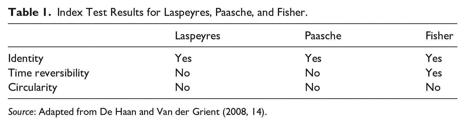
Source: Adapted from De Haan and Van der Grient (2008, 14).

Fisher’s system of tests are mostly included in regulations for official statistics (e.g., Eurostat 2022; ILO et al. 2020). In this paper we, therefore, focus on the identity test, the time reversal test, and the circular test.

2.2. Desired Practical Properties

Looking beyond methodological properties has not always been common. In the last decade, attention for the practical side, however, grew. In its “Quality Framework and Guidelines for OECD Statistical Activities,” the OECD stated that “Quality is defined as ‘fitness for use’ in terms of user needs” (OECD 2012, 7). It is also the first principle in the UN’s “Fundamental Principals of Official Statistics” that “official statistics should meet the test of practical utility” (UN 2014, 2). For successfully compiling official statistics, it is, therefore, recommended to also consider practical components.

The first practical property, we denote in this study, is a stable index. If price developments go up for 10% in one period and go down by 20% in the next period, it is difficult for users to assess how the market is evolving. The aim for index construction is, however, not to remove market volatility, but only to remove volatility that is intrinsic to the index method or non-existing volatility. The more existing volatility is removed, the more it leans toward smoothing. Over the years, this trade-off has been discussed in various studies. Silver (2016) warns for the effects of adding stability trough smoothing. He states that there is a loss of credibility if apparent volatility is not mirrored in the index. Schwann (1998) also mentions disadvantages of forcing stability and acknowledges there is a trade-off: smoothing in essence is undesirable, because it will deviate from the true (to be estimated) index. On the other hand it enhances accuracy (an elaboration on this is provided in Subsection 3.3). Both authors seem to refer to real market volatility and not volatility that is intrinsic to the method. On the other hand, smoothing has at least two advantages: making the underlying trend visible and averaging inaccurate estimates. Regarding the latter, Francke (2010) explains how index modeling can lead to volatility. If regression models are used, the estimated regression coefficient is sensitive to transaction noise. In broad pricing context, noise refers to information that misrepresents the underlying trend. This is caused by the coincidental distribution of observed prices across periods. As a consequence, observed transaction prices differ from its true (and to be estimated) market prices and thus, basing an index on only observed prices can lead to inaccurate estimates. Regarding trends, from the perspective of official statistics, in the CPI manual it is stated that for some purposes, “measuring core inflation is desirable from an economic stance” and “central banks use measures of the general trend of inflation when setting monetary policy” (ILO et al. 2020, 329). In CPIs, core inflation is commonly captured by excluding prices of items that are deemed volatile. In other words, these are items that are susceptible to short-term shocks (ILO et al. 2020, 30). Measuring core inflation, in that sense, aligns with the goals of our study. Given that banks will be main users of CPPIs, this argues for the use of an indicator that captures the trend, but not the volatility. From these perspectives, estimating true market prices is favorable, but it should be done with cautiousness not to remove useful market information.

The second practical property is to create an index that is not overly subject to revision. To be clear, we are not talking about revisions due to mistakes, but revision that are inherent to the index method. Index methods that suffer from this issue are, for example, hedonic time dummy and repeat sales. Every time a new period is added, the model has to be re-estimated and it leads to changes to the entire—previously estimated—index series. In its guideline on revision policy for Principal Economic Indicators (PEEIs: indicators which are essential for monitoring, such as real estate prices), Eurostat (2013a, 5) states that “revisions are something of a double-edged sword.” The estimation is improved, but if it results in “a different assessment of the state of the economy,” it can “damage the credibility of the statistical data.” In addition, from a user’s perspective, “too many revisions create uncertainty” (Eurostat 2013a, 7). Silver (2016, 20), however, states that a “problem” with the revision “should not be overstated” as there are many real estate price indices in the Unites Stated that suffer from continuous revision and it is without any complaints of users. Clapham et al. (2006), on the other hand, state that “index stability” (in terms of limited revisions) is often overlooked in index construction. Given the wide use of real estate indices, limiting revisions is highly relevant. Deng and Quigley (2008) provide further explanation: the initial estimations of real estate price indices are mostly used. If a month later the initial estimation is revised, people don’t pay much attention to the revision as the focus is on the price development of the most recent period. Revisions, therefore, are mostly informational. Moreover, if revisions tend to be large, the usefulness of the index becomes compromised. Therefore EU member states are by legislation bound to only one preliminary period for the House Price Index (HPI) (European Union 2023). Given that development of HPIs is more advanced than CPPIs, CPPIs can be expected to have the same restrictions in the future. From these perspectives, it can be concluded that limited revision of an index is favorable, but there should be awareness not to give in on accurateness.

The third property is the ability of detecting turning points in an early stage. An early detection of turning points has the particular interest of users involved in management in the real estate economy. In the use of CPPIs, “the focus of much of the analysis . . . is on trends and turning points. In this context users need regular and timely data . . . for the detection and identification of economic relationships” (Eurostat 2017, 27). A turning point is, in this study, defined as a “structural” change in the price development from positive to negative or the other way around. The term “structural” closely relates to the first property of a stable index. In a volatile index, changes from positive to negative occur often. Structural changes are, therefore, hard to detect in an unstable index. Some cautiousness is, however, appropriate in making indices more stable by smoothing. Eurostat (2017, 120) notes “late detection or turning points due to systematic smoothing of the index” as a potential issue. The type of smoothing that is referred to is, however, caused by using valuations as data source rather than smoothing as a method. Hill and Steurer (2020) and Francke (2010) then again, notice that certain index models (namely Repeat Sales models) can also cause lags, which prevents an early detection of turning points.

3. Methodology

There are several possible approaches in constructing a price index for small, heterogeneous domains that meet the most desired practical and methodological properties. In this study, we propose a four-step procedure. We base each of these steps on existing techniques, which we alter for our present purpose. In sequential order, these steps are (1) hedonic imputations, (2) multilateral imputations, (3) time series re-estimated imputations, and (4) window splicing. This is the first study that combines above techniques to construct a price index. An overview of the steps and summary of the effects is provided in Figure 1. Each step is discussed in detail in Subsections below.

Figure 1.

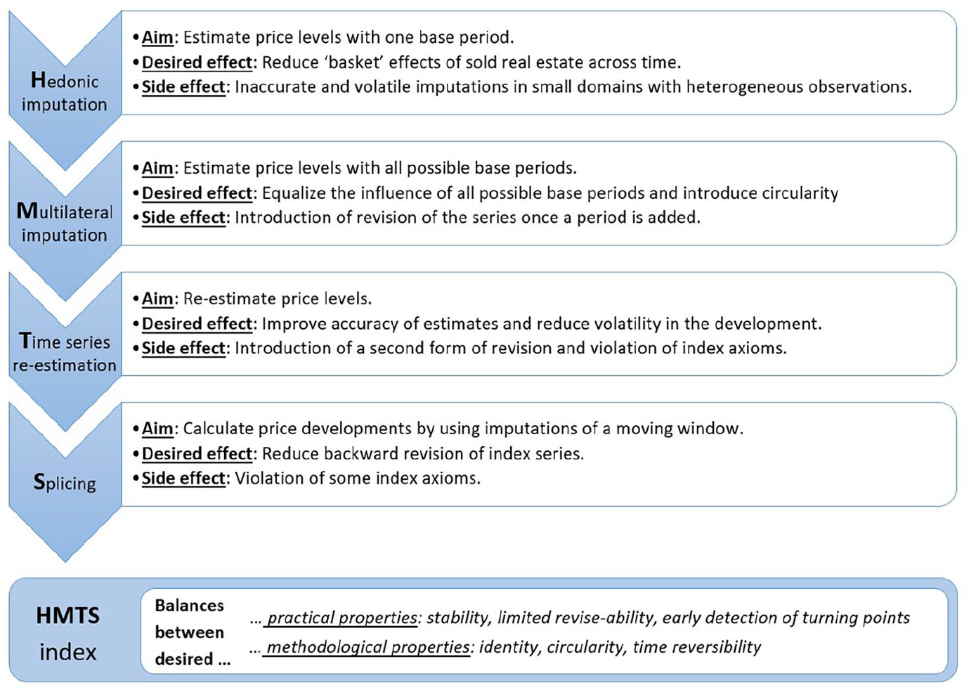
HMTS procedure.

3.1. Step 1: Hedonic Imputations

The aim for a Commercial Property Price Index (CPPI) is a constant quality price index. In other words, the purpose is to measure pure price changes of real estate and not changes in quality. Therefore, a comparison of sold real estate between periods should be adjusted for changes in quality between the periods. For the measurement of non-durable goods, this is less of an issue as the exact same product can be purchased in succeeding periods. For real estate this is problematic, because every real estate object is unique and, in every period, a different selection of real estate is sold. As a first step, hedonic regression is introduced in this procedure to adjust for the quality changes between periods. Hedonic regression is in essence a breakdown of complex good (such as real estate) into its components. These are, for example, size, location, building age, and so on. The composition of a hedonic model is actually a very important, but different topic. The hedonic model should contain important and statistically significant attributes of real estate prices and the assumptions for hedonic modeling should be tested. Miyakawa et al. (2024), for one, show the diversity of attributes that could be taken into account for explaining commercial transaction prices. Once the model is adequately formed, one can proceed to the next step.

The value or sale price can be expressed as an additive function of these characteristics. Linear regression (OLS: Ordinary Least Squares) is used to an averaged value addition for all components. These averages are then used to calculate model prices or imputed prices for each observation. A common logarithmic-linear model, based on Eurostat (2013b, 50), which is used to calculate the averaged value additions $(β)$ per period, is:

l n p_{t}^{i} = β_{t} + \sum_{k = 1}^{K} β_{t}^{k} x_{t}^{i k} + ε_{t}^{i},

(1)

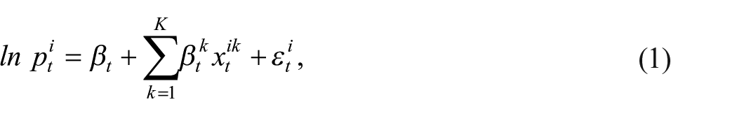
where:

${p^{i}}_{t} = t h e p r i c e o f t h e i^{t h} p r o p e r t y s o l d i n p e r i o d t;$

$β_{t} = the intercept term in period t;$

$β_{t}^{k} = the coefficient of the k^{t h} characteristic in period t;$

$x_{t}^{i k} = the k^{t h} characteristic of the i^{t h} property sold in period t;$

$ε_{t}^{i} = a random error term of the i^{t h} property sold in period t, with ε_{t}^{i} ~ N (0, σ) .$

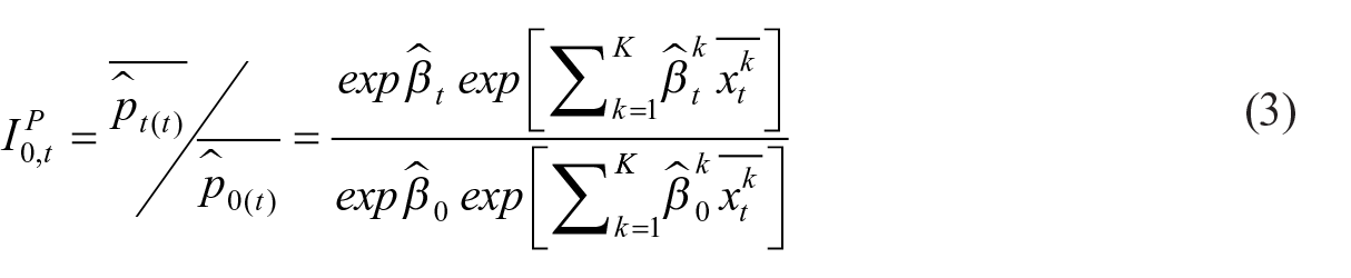
To understand the application of above regression in the HMTS method, it helps to first understand the basics of the Laspeyres and Paasche hedonic double imputation (HDI) method. In both methods, the regression is run for each period, and the model prices are estimated (or imputed) with the retrieved intercept and coefficients. The difference between the two is the base period. In Laspeyres indices, the characteristics of the first period are kept constant. In Paasche indices, the characteristics of the reporting period are kept constant. The index formulae of both are presented below.

I_{0, t}^{L} = \frac{\bar{{\hat{p}}_{t (0)}}}{\bar{{\hat{p}}_{0 (0)}}} = \frac{e x p {\hat{β}}_{t} e x p [\sum_{k = 1}^{K} {\hat{β}}_{t}^{k} \bar{x_{0}^{k}}]}{e x p {\hat{β}}_{0} e x p [\sum_{k = 1}^{K} {\hat{β}}_{0}^{k} \bar{x_{0}^{k}}]}

(2)

I_{0, t}^{P} = \frac{\bar{{\hat{p}}_{t (t)}}}{\bar{{\hat{p}}_{0 (t)}}} = \frac{e x p {\hat{β}}_{t} e x p [\sum_{k = 1}^{K} {\hat{β}}_{t}^{k} \bar{x_{t}^{k}}]}{e x p {\hat{β}}_{0} e x p [\sum_{k = 1}^{K} {\hat{β}}_{0}^{k} \bar{x_{t}^{k}}]}

(3)

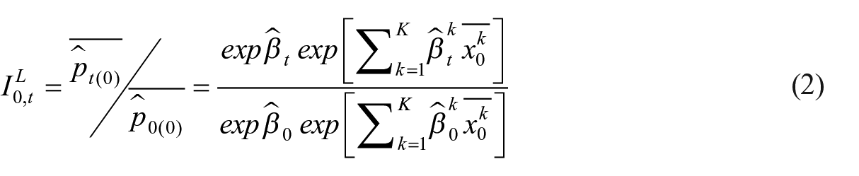
The added terms, compared to Equation (1), are:

$I_{0, t}^{L}$ = Laspeyres HDI price index number between period $0$ and $t$ ;

$\bar{{\hat{p}}_{t (0)}}$ = average imputed price of period t with base period 0;

$\bar{x_{0}^{k}} = average of the k^{t h} characteristic in period 0 . This is calculated by \sum_{i = 1}^{N_{t}} x_{0}^{i k} / N_{0},$

$with N_{0} representing the number of observations in period 0 .$

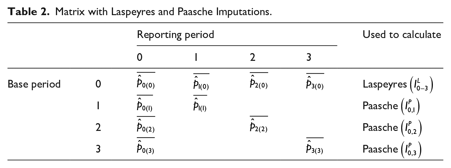
As can be seen, the variations between Laspeyres and Paasche are caused by variating in base periods. In Laspeyres, the characteristics, $\bar{x_{0}^{k}}$ , are kept constant in both the numerator and the denominator at period 0. This results in price imputations, $\bar{{\hat{p}}_{t (0)}}$ , with base period 0. In words, the mix of sold real estate in period 0 is tracked through time. Its prices are imputed in the next periods as if they were sold in another period. These imputations are made by using the regression coefficients, ${\hat{β}}_{t}^{k}$ , which are obtained by Ordinary Least regression (OLS). In the case of Paasche, Equation (3) this is turned around and the mix of sold real estate in period $t$ is tracked through time. A schematic overview of all imputations of four sequential periods (0 < 1 < 2 < 3), required for a Laspeyres and a Paasche index, is provided in the table below.

Note that the Laspeyres index uses only imputations in one row, indicating that there is only one imputation for each period. This is in contrast to the Paasche index that uses imputations in multiple rows, because each addition of a period creates a new version of the imputed price in period 0 $({\hat{p}}_{0})$ . In this study, Equations (2) (Laspeyres) and (3) (Paasche) are not performed to construct the HMTS index. Only the element of imputed prices is used. In Table 2, these are presented as the values for $\bar{\hat{p}}$ .

Table 2.

Matrix with Laspeyres and Paasche Imputations.

		Reporting period				Used to calculate
		0	1	2	3	Used to calculate
Base period	0	$\bar{{\hat{p}}_{0 (0)}}$	$({\hat{p}}_{0})$	$\bar{{\hat{p}}_{2 (0)}}$	$\bar{{\hat{p}}_{3 (0)}}$	Laspeyres $(I_{0 ‒ 1}^{L})$
	1	$\bar{{\hat{p}}_{0 (1)}}$	$\bar{{\hat{p}}_{1 (1)}}$			Paasche $(I_{0, 1}^{P})$
	2	$\bar{{\hat{p}}_{0 (2)}}$		$\bar{{\hat{p}}_{2 (2)}}$		Paasche $(I_{0, 2}^{P})$
	3	$\bar{{\hat{p}}_{0 (3)}}$			$\bar{{\hat{p}}_{3 (3)}}$	Paasche $(I_{0, 3}^{P})$

3.2. Step 2: Multilateral Imputations

Table 2 shows a common characteristic in both the Laspeyres and the Paasche index: there is a large dependency on the imputations in period 0. In the Laspeyres index, period 0 is used as base period and in the Paasche index, the imputations of period 0 are recalculated in each reporting period. Especially when using small datasets, the use of one base period can be perceived as a deficiency as is the case with Laspeyres and Paasche indices. In Laspeyres, the selection of transacted real estate in period 0 is tracked through time in the entire index series. If the data is limited, the possibility grows that this selection does not resemble the stock of real estate or the sold real estate in other periods. In Paasche, the selection of real estate in period t is tracked, but in every calculation, it uses regression results of period 0. If the data is limited, the possibility grows these regression results lack accuracy. A common way to mediate between Laspeyres and Paasche is to calculate a Fisher index, which is the geometric mean of the Laspeyres and Paasche index. As the Fisher index is composed from the Laspeyres and Paasche index, it also inherits the mentioned deficiencies. In all three indices, the choice of base period is arbitrary. To fix this dependency on one or a few base periods, we propose a multilateral approach, which is achieved by filling the blanks in Table 2 as illustrated in Table 3. By completing the matrix, every reporting period is calculated with every possible base period. This results in multiple series and all of these cover the complete time span, hence the term “multilateral.”

Table 3.

Matrix with Multilateral Imputations.

		Reporting period
		0	1	2	3
Base period	0	$\bar{{\hat{p}}_{0 (0)}}$	$\bar{{\hat{p}}_{1 (0)}}$	$\bar{{\hat{p}}_{2 (0)}}$	$\bar{{\hat{p}}_{3 (0)}}$
	1	$\bar{{\hat{p}}_{0 (1)}}$	$\bar{{\hat{p}}_{1 (1)}}$	$\bar{{\hat{p}}_{2 (1)}} *$	$\bar{{\hat{p}}_{3 (1)}} *$
	2	$\bar{{\hat{p}}_{0 (2)}}$	$\bar{{\hat{p}}_{1 (2)}} *$	$\bar{{\hat{p}}_{2 (2)}}$	$\bar{{\hat{p}}_{3 (2)}} *$
	3	$\bar{{\hat{p}}_{0 (3)}}$	$\bar{{\hat{p}}_{1 (3)}} *$	$\bar{{\hat{p}}_{2 (3)}} *$	$\bar{{\hat{p}}_{3 (3)}} *$

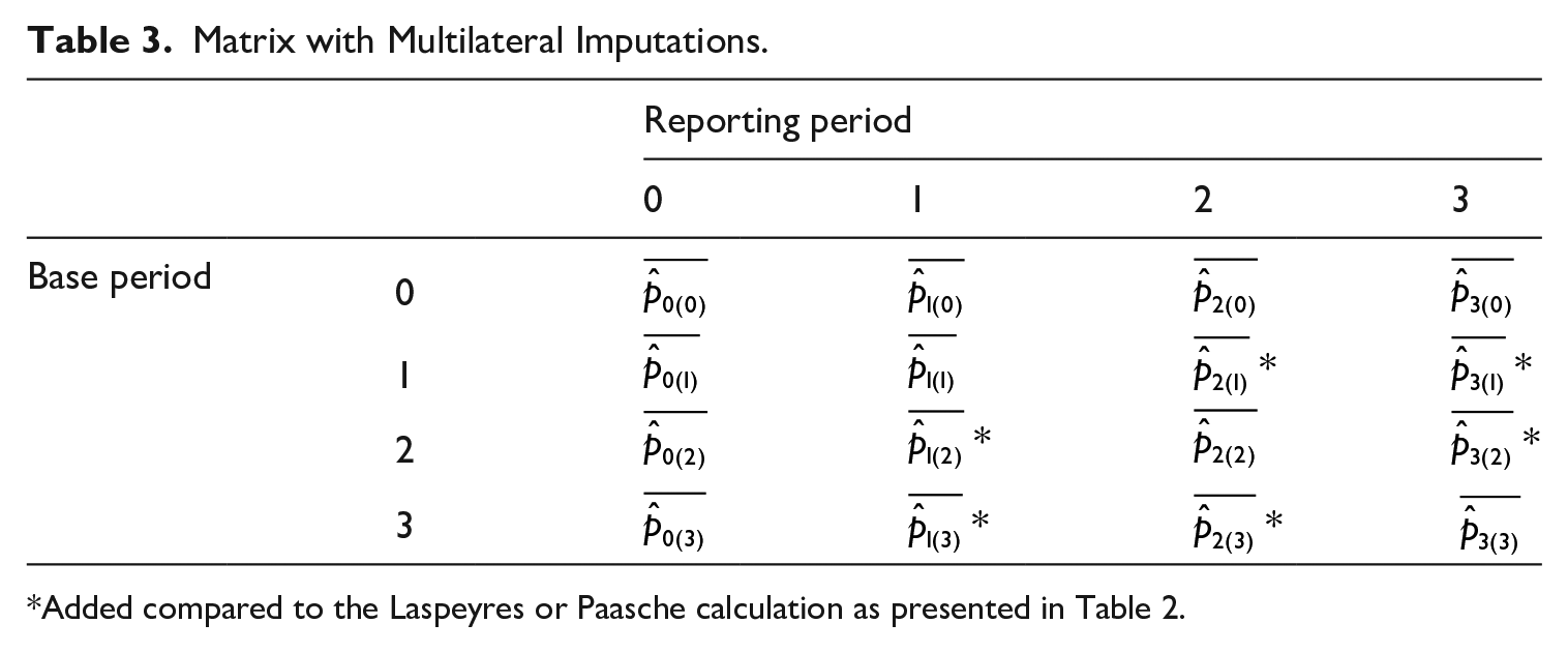
Added compared to the Laspeyres or Paasche calculation as presented in Table 2.

This approach is inspired by the multilateral GEKS (Gini 1931; Eltetö and Köves 1964; Szulc 1964 as referenced in De Haan and Van der Grient 2011) method as described by Willenborg (2017, 2018). In his study, Willenborg explains the GEKS method as completing a matrix with index figures based on all possible base periods. By taking the geometric mean of all possibilities for each reporting period, circularity is realized (Table 1 shows that Laspeyres, Paasche, and Fisher do not pass the circularity test). A direct price development between period 0 and 2 equals a multiplication between direct indices between period 0 and 1 and period 1 and 2. The formula for retrieving each imputation is provided in Equation (4).

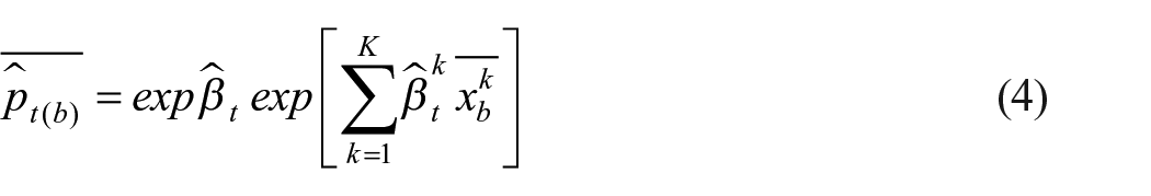
\bar{{\hat{p}}_{t (b)}} = e x p {\hat{β}}_{t} e x p [\sum_{k = 1}^{K} {\hat{β}}_{t}^{k} \bar{x_{b}^{k}}]

(4)

Opposed to Equations (2) and (3), the base periods are flexible as it can have any value between 0 and t. Calculating one single imputation for period t is achieved by taking the geometric mean of all variations with different base periods, illustrated in Equation (5).

\bar{{\hat{P}}_{t}} = {(\prod_{b = 0}^{T} \bar{{\hat{p}}_{t (b)}})}^{1 / T}, w i t h t = 0, 1, \dots, T

(5)

With $\bar{{\hat{p}}_{2 (3)}} *$ , a circular index $\bar{{\hat{p}}_{3 (3)}}$ can be constructed according to Equation (6).

I_{0, t} = \frac{\bar{{\hat{P}}_{t}}}{\bar{{\hat{P}}_{0}}}

(6)

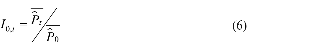
In this study, Equations (5) and (6) are not performed at this stage for the final index. The imputations resulting from Equation (4) are used in the next step.

3.3. Step 3: Time Series Re-Estimated Imputations

The result of Equation (6) is a circular index that does not heavily rely on one base period. However, the individual imputations in step 1 may still lack accuracy and thus a resulting index still shows volatile developments. This is especially the case if hedonic regression is performed on small datasets with a high degree of heterogeneity. Time series analysis, and in particular state space modeling is used in this step to improve the price imputations in terms of accuracy, reliability, and validity. A few notes on the latter concepts seem appropriate at this point and Babbie (2014, 140–3) provides definitions that we will use to describe how time series re-estimations will enhance the index.

Accuracy often refers to the proximity of a measurement to the true value. As we are aiming for trend like behavior of the price developments, moving away from volatility seems to add accuracy. This is not to be confused with precision. Precision reflects the closeness of multiple observations to each other. For example, estimating a man as “thirty-six years old” is more precise than “in his thirties.” If the man is in fact thirty-nine years old, the latter estimation is, however, the only accurate one. In our case, the introduction of time series re-estimations adds accuracy, but hands in on precision.

Reliability refers to whether a technique, applied repeatedly to the same observation, yields the same result. The re-estimation reduces volatility and, therefore, also variance in outcome. This leads to more similar results when simulations are run with in-sample variations. This analysis is further described in Subsection 4.2 (Figure 5—confidence intervals).

Validity refers to the extent to which a measure reflects the real meaning of the concept. The concept we are aiming to measure is price developments in the real estate market. Again here, volatility prevents us from capturing the real underlying market developments. Due to low numbers and heterogeneity, a volatile index rather captures momentarily developments of incidental transactions.

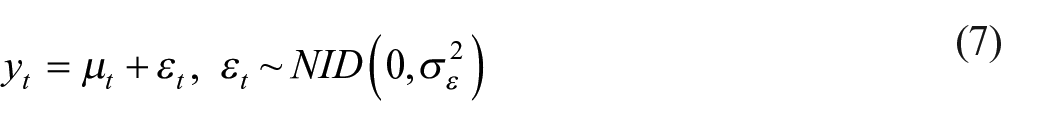
In time series analysis, all values in the series are assumed to be related, that is, there is a correlation between adjacent periods. State space models make a general distinction between observed and unobserved variables. The former is model input and the latter is model output. A simple state space model (in this case a random walk plus noise model) is represented in Equations (7) and (8) (Commandeur and Koopman 2007, 9).

y_{t} = μ_{t} + ε_{t}, ε_{t} ~ N I D (0, σ_{ε}^{2})

(7)

μ_{t + 1} = μ_{t} + ξ_{t}, ξ_{t} ~ N I D (0, σ_{ξ}^{2})

(8)

The terms in this formula are:

$y_{t}$ = the observed value in period t;

$μ_{t}$ = the unobserved level in period t;

$ε_{t} = the observation disturbance in period t;$

$ξ_{t} = the level disturbance in period t;$

$N I D () indication that the disturbance terms are normally and independently distributed .$

Equation (7) is called the measurement or observation equation. It separates the observed series $y_{t}$ into a signal $(μ_{t})$ and a noise component. The essence of above model is that the signal is described by a series of unobserved states mt that evolve through time. This is done by the second Equation (8), called the transition equation. It describes how the unobserved state mt depends on the previous value of mt. The amount of change between consecutive values of mt is determined by a series of random shocks $ξ_{t}$ .

We are interested in the unobserved states and are able to estimate these with help of the observed series. In our case, the observed states $y_{t}$ refer to the estimated average hedonic price levels, resulting from Equation (5). Following Equation (7), we assume the series of observed price levels $y_{t}$ contain noise or observation disturbances. The state space assumption is that we cannot observe the true states (unobserved levels) directly and these should be estimated.

Regarding reducing volatility, these state space methods as described by Commandeur and Koopman (2007) and Durbin and Koopman (2012), show great potential, because the unobserved levels tend to be smoother than the observed levels. With the assumption that there is correlation within the time series, the estimated unobserved levels are most likely also more accurate estimates of the price developments. Francke and de Vos (2000), Francke (2010), Rambaldi and Fletcher (2014), and Hill et al. (2021) already proved that integration of hedonics and state space methods can result in stable estimates of growth rates.

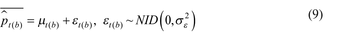
After Equation (8), there are many different models to choose from. In our study, many models were tested and the best model was chosen by looking at the most suitable fit. The model showed, among which, the lowest AIC (presented in Appendix 2). The model of choice is a local linear trend model. In this model, another term, the slope component, is introduced to further improve the estimation of the trend. In general, the addition of a slope is more suitable for long term and changing trends. Furthermore, the model sets a hyperparameter of the level component equal to zero, while the slope component remains stochastic. This model is also known as a smooth trend model, and since the slope disturbances affect the level component indirectly, generally yield a smoother estimate of the level component. Equations (9) to (11) represent this model applied to the price imputations resulting from step 2.

\bar{{\hat{p}}_{t (b)}} = μ_{t (b)} + ε_{t (b)}, ε_{t (b)} ~ N I D (0, σ_{ε}^{2})

(9)

μ_{t + 1 (b)} = μ_{t (b)} + v_{t (b)}

(10)

v_{t + 1 (b)} = v_{t (b)} + ζ_{t (b)}, ζ_{t (b)} ~ N I D (0, σ_{ζ}^{2})

(11)

The added terms in this formula are:

$\bar{{\hat{p}}_{t (b)}}$ = the imputed price of reporting period $t$ with base period $b$ (observed values);

$μ_{t (b)}$ = the unobserved level in period t for the series with base period $b$ ;

$v_{t (b)} = the slope component in period t (deterministic) for the series with base period b;$

$ζ_{t (b)} = the slope disturbance in period t for the series with base period b .$

In Equation (9), the observed values $y_{t}$ are replaced by the imputed prices $\bar{{\hat{p}}_{t (b)}}$ retrieved from the previous step. Opposed to Equation (8), the estimation of $μ_{t (b)}$ is now expanded with slope $v_{t (b)}$ in Equation (10). Slope $v_{t (b)}$ depends in its turn on the previous estimation of $v_{t (b)}$ . The model can be estimated by applying a two-step procedure. First, the hyperparameters, that is, the variances of the error terms, are estimated via a Maximum Likelihood procedure. Then the Kalman filter (Kalman 1960) is applied to estimate the state variables (level and slope). The Kalman filter is a recursive algorithm that first applies a forward pass to the time series, from t = 1 to t = T, and at each step updates the estimates of the state variables. This is called filtering. The estimates at time t are thus only based on information up to that period. Then a backward pass is applied from t = T to t = 1, in which the filtered estimates are updated using all available information. This is called smoothing. In our case we are interested in these smoothed estimates, since this is the added value of step 3 (capturing the trend). Once the model is estimated, the re-estimated imputations can be derived as follows.

\tilde{\bar{{\hat{p}}_{t (b)}}} = \hat{μ_{t (b)}} = \bar{{\hat{p}}_{t (b)}} - \hat{ε_{t (b)}}

(12)

The term $\tilde{\bar{{\hat{p}}_{t (b)}}}$ represents the re-estimated price imputation in period t with base period b. A schematic overview of all re-estimated price levels of four sequential periods (0 < 1 < 2 < 3) with the same number of base periods is provided in Table 4.

Table 4.

Matrix with Re-Estimated Multilateral Imputations.

		Reporting period
		0	1	2	3
Base period	0	$\tilde{\bar{{\hat{p}}_{0 (0)}}}$	$\tilde{\bar{{\hat{p}}_{1 (0)}}}$	$\tilde{\bar{{\hat{p}}_{2 (0)}}}$	$\tilde{\bar{{\hat{p}}_{3 (0)}}}$
	1	$\tilde{\bar{{\hat{p}}_{0 (1)}}}$	$\tilde{\bar{{\hat{p}}_{1 (1)}}}$	$\tilde{\bar{{\hat{p}}_{2 (1)}}}$	$\tilde{\bar{{\hat{p}}_{3 (1)}}}$
	2	$\tilde{\bar{{\hat{p}}_{0 (2)}}}$	$\tilde{\bar{{\hat{p}}_{1 (2)}}}$	$\tilde{\bar{{\hat{p}}_{2 (2)}}}$	$\tilde{\bar{{\hat{p}}_{3 (2)}}}$
	3	$\tilde{\bar{{\hat{p}}_{0 (3)}}}$	$\tilde{\bar{{\hat{p}}_{1 (3)}}}$	$\tilde{\bar{{\hat{p}}_{2 (3)}}}$	$\tilde{\bar{{\hat{p}}_{3 (3)}}}$

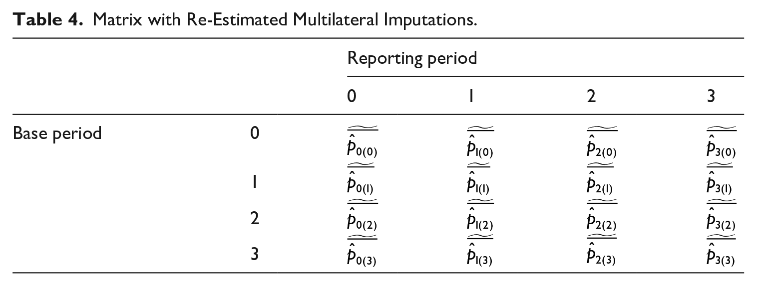
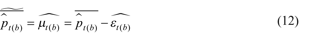
From these re-estimated imputations, an index can be constructed according to Equations (5) and (6). In this study, Equations (5) and (6) are not performed at this stage for the final index. The imputations resulting from Equation (12) are used in the final step.

3.4. Step 4: Window Splice

At this point in the procedure, the method is expected to provide more stable indices. However, the other practical property of limited revisions is not met. The previous steps of multilateral calculations and time series re-estimations both cause revisions once a period is added.

For multilateral calculations the mechanism is as follows: once a reporting period is added, a series is added with another base period. This is demonstrated in Table 3: adding a column (reporting period) also means adding a row (series with upgraded base period). Calculating the geometric mean of all possibilities for period 0, now includes one extra figure (with base period t). This occurs in all periods and therefore the figures of all periods are revised.

For the time series re-estimations, the mechanism is as follows: once a reporting period is added, the calculation of the previous period is adjusted as each unobserved value is calculated with information of the preceding and succeeding period. This occurs in all periods and therefore the figures of all periods are revised.

A rolling window approach or window splicing is introduced in this study to avoid revision of the entire series every time a reporting period is added. As shown by Shimizu et al. (2010), Ivancic et al. (2011), Krsinich (2016), Chessa (2021), Bentley (2022), and Diewert and Fox (2022), splicing is well known in index construction, especially in combination with multilateral methods. Hill et al. (2022) report that the technique is also widely used in official statistics (at least in the form of a rolling time dummy method). The main idea of window splicing is to keep a limited number of periods provisional instead of the entire time series. To bypass the revisions caused by the multilateral calculations, the final averaged index number is not based on all possibilities of an imputed price, but on a selection.

This selection is performed in a two-step procedure. First, to bypass the revisions caused by the multilateral time series re-estimation, the series for each base period will not endlessly be updated. An example to illustrate this: a window is determined at three periods. In other words, once period $t$ is calculated for the first time it is provisional. In this period and the next two periods, the figure for period $t$ is subject to revision. In period $t + 1$ , the series with base period $t$ is extended with reporting period $t + 1$ . In period $t + 2$ , the series with base period $t$ is extended again with reporting period $t + 2$ . In both calculations, the figure for period $t$ is revised. This will be the last time, since the series with base period $t$ is fixed from that point on. An illustration of this update scheme is provided in Table 5.

Table 5.

Matrix with Update Scheme of Re-Estimated Multilateral Imputations.

		Reporting period
		0	1	2	3	4	5
Base period	0	$\tilde{\bar{{\hat{p}}_{0 (0)}}}$	$\tilde{\bar{{\hat{p}}_{1 (0)}}}$	$\tilde{\bar{{\hat{p}}_{2 (0)}}} *$
	1	$\tilde{\bar{{\hat{p}}_{0 (1)}}}$	$\tilde{\bar{{\hat{p}}_{1 (1)}}}$	$\tilde{\bar{{\hat{p}}_{2 (1)}}}$	$\tilde{\bar{{\hat{p}}_{3 (1)}}}$
	2	$\tilde{\bar{{\hat{p}}_{0 (2)}}}$	$\tilde{\bar{{\hat{p}}_{1 (2)}}}$	$\tilde{\bar{{\hat{p}}_{2 (2)}}}$	$\tilde{\bar{{\hat{p}}_{3 (2)}}}$	$\tilde{\bar{{\hat{p}}_{4 (2)}}}$
	3	$\tilde{\bar{{\hat{p}}_{0 (3)}}}$	$\tilde{\bar{{\hat{p}}_{1 (3)}}}$	$\tilde{\bar{{\hat{p}}_{2 (3)}}}$	$\tilde{\bar{{\hat{p}}_{3 (3)}}}$	$\tilde{\bar{{\hat{p}}_{4 (3)}}}$	$\tilde{\bar{{\hat{p}}_{5 (3)}}}$
	4	$\tilde{\bar{{\hat{p}}_{0 (4)}}}$	$\tilde{\bar{{\hat{p}}_{1 (4)}}}$	$\tilde{\bar{{\hat{p}}_{2 (4)}}}$	$\tilde{\bar{{\hat{p}}_{3 (4)}}}$	$\tilde{\bar{{\hat{p}}_{4 (4)}}}$	$\tilde{\bar{{\hat{p}}_{5 (4)}}}$
	5	$\tilde{\bar{{\hat{p}}_{0 (5)}}}$	$\tilde{\bar{{\hat{p}}_{1 (5)}}}$	$\tilde{\bar{{\hat{p}}_{2 (5)}}}$	$\tilde{\bar{{\hat{p}}_{3 (5)}}}$	$\tilde{\bar{{\hat{p}}_{4 (5)}}}$	$\tilde{\bar{{\hat{p}}_{5 (5)}}}$

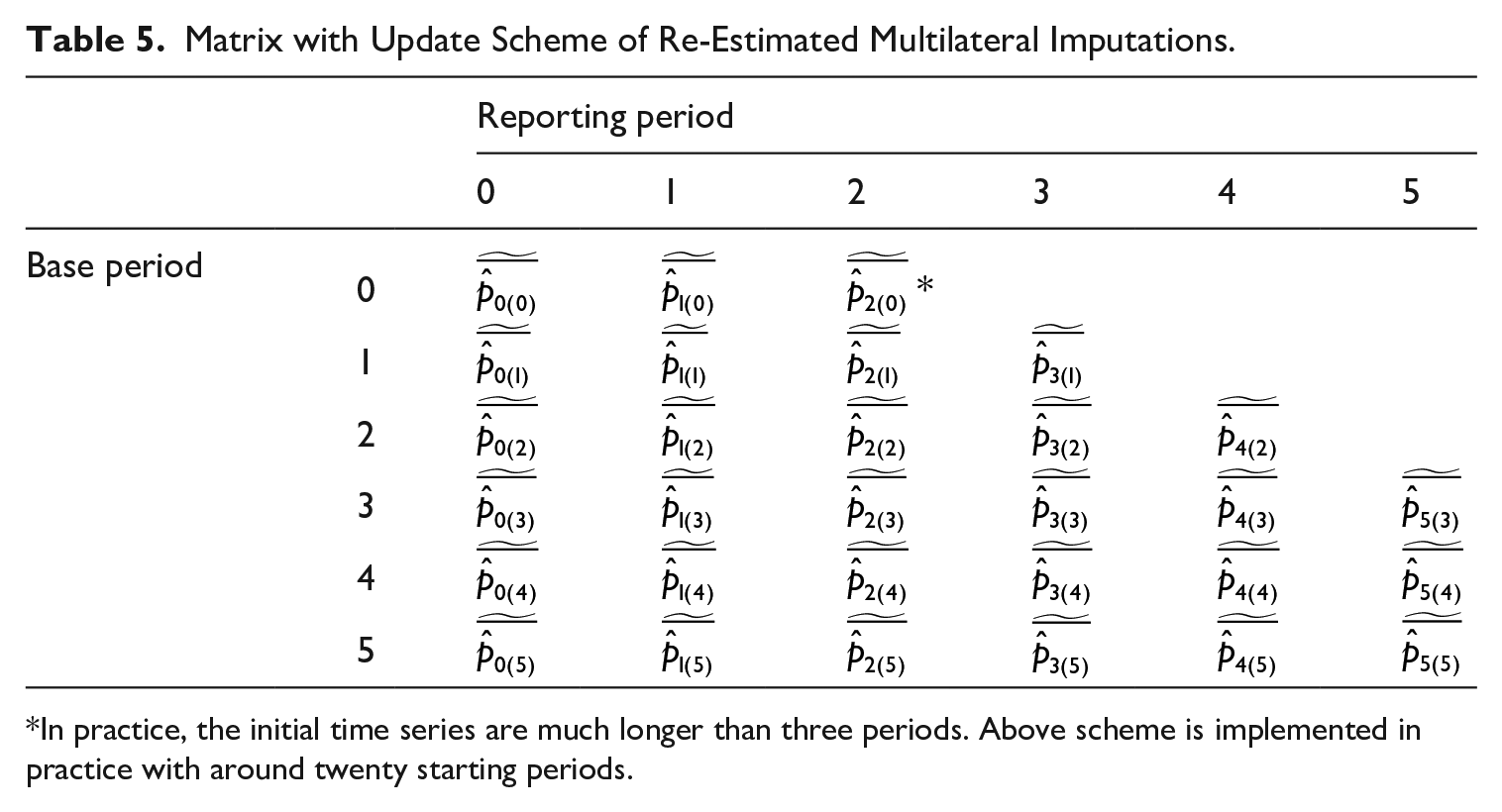
In practice, the initial time series are much longer than three periods. Above scheme is implemented in practice with around twenty starting periods.

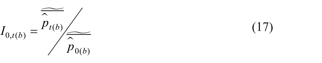
Second, the above imputations are transformed into index figures. This is achieved by dividing the imputation of the reporting period by the imputation of the first period as shown in Equation (17). At this point, a transformation into indices is necessary, because in the next step—Equation (18)—, the multilateral series, all with different base periods, are merged into final index figures. The imputations, presented in Table 5, are comparable over time within its own series using its own base period. The imputations are not comparable over time across different base period series. A transformation into index figures makes the series comparable and ready for the final step.

I_{0, t (b)} = \frac{\tilde{\bar{{\hat{p}}_{t (b)}}}}{\tilde{\bar{{\hat{p}}_{0 (b)}}}}

(17)

After the index transformation, the windows are created. The final index is the geometric average of a window of index mutations. For example, if the window length is three periods, the index figure of reporting period $t$ ( $I_{0, t}$ ) is the geometric average of the indices with base period $t - 2$ until base period $t$ : $I_{0, t (t - 2)}$ , $I_{0, t (t - 1)}$ , and $I_{0, t (t)}$ . The formula to construct the price index according to the proposed method multilateral hedonic imputation with time series re-estimation and window length $w$ , is provided in equation (18).

I_{0, t}^{M H I T - w} = {(\prod_{b = t - (w - 1)}^{T} I_{0, t (b)})}^{1 / w}, w i t h t = w - 1, w, \dots, T

(18)

Above formula is not applied to the first set of windows as this would imply that first windows would be based on fewer periods then the window length. For example, following Equation (18) for reporting period 0, would result in a window from period −2 to 0. Since there are no negative periods, period 0 remains and the window would include just one period. To solve this, the first windows ( $t < (w - 1)$ ) are calculated with altered Equation (19).

I_{0, t}^{M H I T - w} = {(\prod_{b = 0}^{w - 1} I_{0, t (b)})}^{1 / w}, w i t h t = 0, \dots, w - 2

(19)

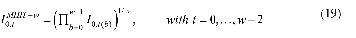
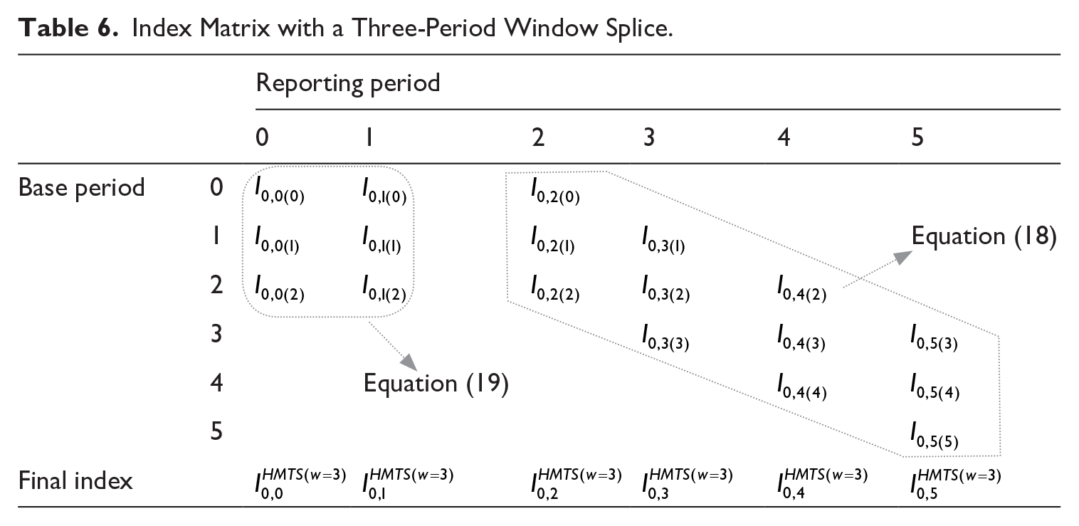
Table 6 illustrates a window splice of three periods and the calculation of the final index. The resulting index is from now on referred to as the HMTS method (Hedonic Multilateral Time series Splice). At this point, the choice of a three period window splice is purely for illustration purposes. The choice of window length is rather important in the index construction. Bentley (2022), for one, acknowledges this and notices that there are no criteria set in official statistics to determine a window length (other than that is should yield reasonable results). He also lists arguments in favor of a shorter or longer window. The most important one, in case of the HMTS, is that greater transitivity goes along with a longer window. On the other hand, a shorter window minimizes the number of revisions. Hill et al. (2022) point out that a longer window generally increases the robustness of the index, while a shorter window increases the current market relevance. They also present a method to determine the optimal length of a window. Another way to look for an optimal window length—and specifically applied to the HMTS—is presented in section 4.2.

Table 6.

Index Matrix with a Three-Period Window Splice.

		Reporting period
		0	1	2	3	4	5
Base period	0	$I_{0, 0 (0)}$	$I_{0, 1 (0)}$	$I_{0, 2 (0)}$
	1	$I_{0, 0 (1)}$	$I_{0, 1 (1)}$	$I_{0, 2 (1)}$	$I_{0, 3 (1)}$		Equation (18)
	2	$I_{0, 0 (2)}$	$I_{0, 1 (2)}$	$I_{0, 2 (2)}$	$I_{0, 3 (2)}$	$I_{0, 4 (2)}$
	3				$I_{0, 3 (3)}$	$I_{0, 4 (3)}$	$I_{0, 5 (3)}$
	4		Equation (19)			$I_{0, 4 (4)}$	$I_{0, 5 (4)}$
	5						$I_{0, 5 (5)}$
Final index		$I_{0, 0}^{H M T S (w = 3)}$	$I_{0, 1}^{H M T S (w = 3)}$	$I_{0, 2}^{H M T S (w = 3)}$	$I_{0, 3}^{H M T S (w = 3)}$	$I_{0, 4}^{H M T S (w = 3)}$	$I_{0, 5}^{H M T S (w = 3)}$

4. Data and Empirical Findings

The analyses in this section are presented and assessed by the practical and methodological properties in below paragraphs. We will present results for our four-step approach, and for each of these steps compare the outcomes to results from the standard approach where only the first step is applied, that is, a hedonic imputation method such as Laspeyres or Paasche index is computed. First, a description of the data is provided.

4.1. Data: Office Building Transactions in the Netherlands

To test the index procedure, data on commercial real estate in the Netherlands is used. The data consists of transactions that are reported on a quarterly basis and span the years of 2008 until 2022. As the focus of this study is on small domains, we selected the subgroup of office buildings—containing limited numbers of observations—to run the calculations. The number of observations ranges from approximately 150 to 1,100 per quarter. These data are also used by Statistics Netherlands to calculate the published CPPIs and have already been cleaned. The cleaning process comprises of correcting data errors, excluding false observations and transforming portfolio sales into useable transactions (CBS 2022). The hedonic variables—as used by Statistics Netherlands for a Fisher Hedonic Double Imputation (HDI) method—were used as input for the hedonic model in step 1. The regression model and its results are enclosed in Appendix 1. The time series analyses results are enclosed in Appendix 2.

The HMTS method relies on a solid hedonic model. Running hedonic diagnostic tests prior to implementing the HMTS method is, therefore, required. Analyses show, however, that the HMTS method performs well even with the most basic hedonic variables: floor area, location, and building age. The results of an index with these variables resembles an index with many additional variables.

4.2. Results Step 1 to 4

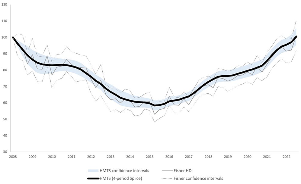
The HMTS index with three preliminary periods (four period window splice) is presented in Figure 2. The stepwise results (from H to HMTS) show that the index corrects for quality changes, detaches from one base period, adds stability and is has a limited revision.

Figure 2.

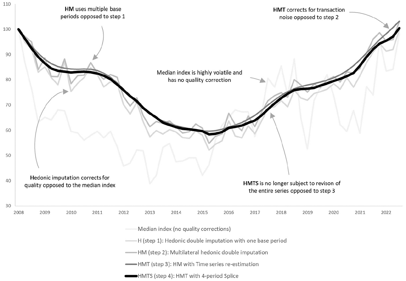
From median index to HMTS index.

4.3. Assessment of Practical Properties

To assess the HMTS index on revisions and the ability to detect turning points, the years around 2015 are more closely analyzed. Both the Fisher HDI and HMTS detect a downward peak in 2015 Q2 (lowest point) and a first rise in 2015 Q3. The latter period is, therefore, marked as a turning point. Figure 3 shows the results of a simulation between 2014 and 2016. The index is calculated with three preliminary periods. Each index point, therefore, has four estimations:

- The first estimation is made in the corresponding calculation period;

- The second estimation is made once the calculation period is one period ahead;

- The third estimation is made once the calculation period is two periods ahead;

- The final estimation is made once the calculation period is three periods ahead.

In this turbulent period, including a turning point, the first estimations are on average 0.82 index point off from the final estimation. As expected, the revision decreases at the second (0.29) and third (0.03) estimation. Given that, the index figures are only subject to a very slight revision after the third estimation, two or three preliminary periods seem to be appropriate in the HMTS index construction.

Figure 3.

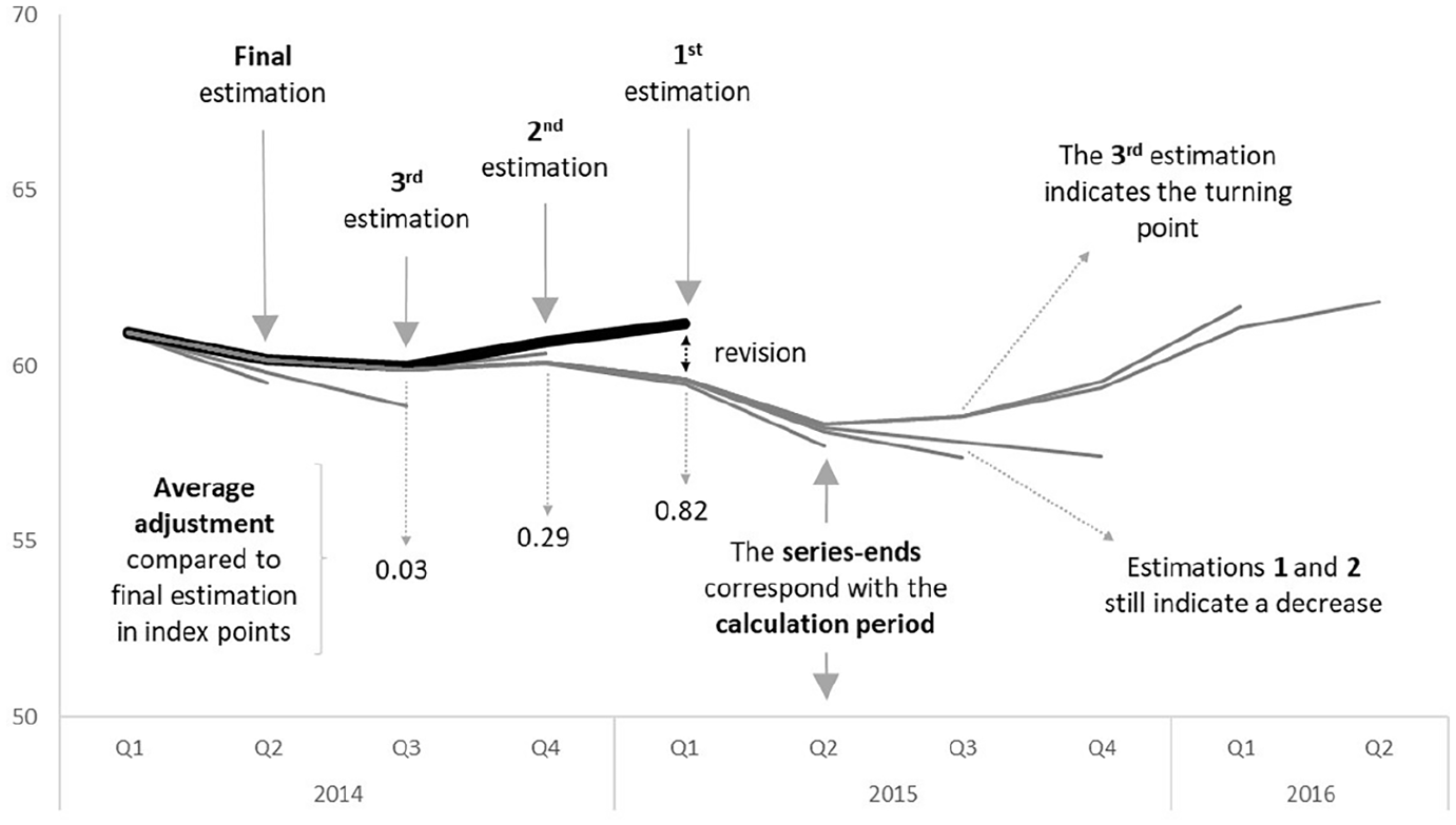
Revisions and turning point detection.

Although the turning point is in the second quarter of 2015 and the index should show an increase, the first two estimations of the HMTS index indicate a downward development. The third estimation is corrected upwards, indicating a turning point. After the revisions the index gets more accurate and above simulation shows that the desired accuracy lags two periods. Even though the HMTS index does not indicate the turning point immediately, the turning was expected after looking at the mutations. Figure 4 shows the changes compared to the same quarter of the previous year for the HMTS index and the Fisher HDI index. Because of the trend-like development of the HMTS index, a clear development toward a turning point can be distinguished. The Fisher index, on the other hand, shows a distorted development.

Figure 4.

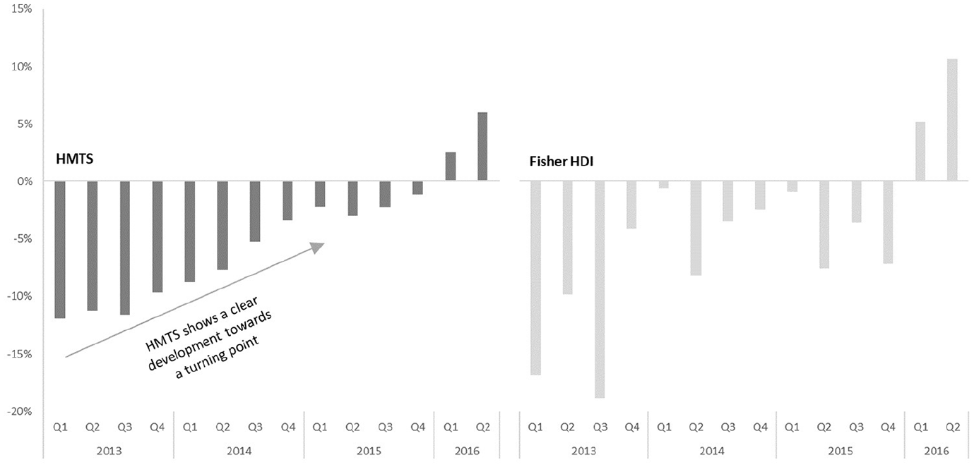
Changes compared to the previous year (%).

To assess the HMTS index on its reliability, stability, and robustness, confidence intervals were calculated. The interval was calculated according to the bootstrap method as described by Efron and Tibshirani (1994) and executed by Johnson (2001) and Willenborg and Scholtus (2018). In essence, the intervals are obtained by simulating variations, using the variability in the data. The index series are calculated five hundred times and, in each calculation, the original input is altered by sampling with replacement until the original sample size is reached. Calculating the variance of the five hundred index series allows us to construct confidence interval as presented in Figure 5. It shows that the HMTS has an improved reliability compared to a Fisher HDI.

Figure 5.

Confidence intervals (95%).

The robustness of the index is also tested by running calculations on a randomly selected subset of the data with fifty observations per quarter. The result, presented in Figure 6, shows that the index is somewhat less stable than the original one (yet not extremely) and in certain years the trend is slightly different. For comparison purposes, the Fisher index is also calculated with the same reduced dataset. It shows that reducing observations, causes more peaks, which indicates the presence of transaction noise.

Figure 6.

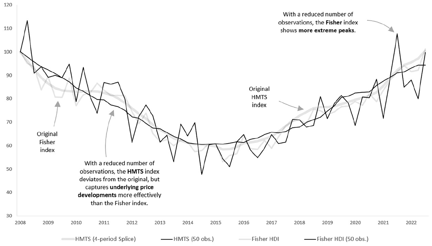
Simulation with fifty observations.

Yet, another way to get an idea of the robustness of the index is to calculate the share of each observation in the index mutation. This type of calculation is often used in official statistics to detect suspicious observations, which should be (manually) checked. The approach to calculate the shares is similar to the bootstrap simulation: the index is calculated as many times as there are observations, and each iteration observations are alternately excluded. This way, the effect of each observation becomes visible by comparing the alternative index to the original index. Calculations performed on the Fisher HDI and the HMTS shows that the range at which observations affect the index decreases with approximately 50%. In the Fisher HDI, the observation’s share in the index ranges from −0.67 to 0.27 index point. On average, the absolute share of individual observations in the index is 0.06 index point. In the HMTS, shares range from −0.4 to 0.2 index point. On average, the absolute share of individual observations in the index is 0.03 index point.

4.4. Assessment of Methodological Properties

The identity test states that once the prices of period t return to the state of period 0, the index should also return to 100. Due to the multilateral approach, the re-estimations, and window splicing, the identity test does not hold anymore in its strict form. That is, if the prices in the data return to the state of period 0, the index does not (necessarily) return to 100. Only in the scenario where all multilateral re-estimations return to the state of period 0, the index does return to 100. This resembles the multiperiod identity test as described by Diewert (2020). In most cases, however, even though the observed prices of both periods are the same, the transaction noise in period 0 will likely differ from the noise in period t. This is because the noise is determined with help of the adjacent periods. Since the adjacent periods differ, so will the noise. Figure 7 shows an empirical test: the prices from period 2020 Q1 and onward are set to the state of 2008 Q1. As illustrated, the Fisher index returns immediately to 100. The HMTS index returns very slowly to the original state. The question here is whether the development of the Fisher index is realistic. The prices of period 2020 Q1 indicate that the prices suddenly peak, but the re-estimations method uses information from other periods as well. The HMTS index, therefore, indicates that a sudden increase is not realistic, but if the prices keep indicating this level, the index eventually returns to the same level. The size of lag depends on the size of the development. Below example could be considered extreme. To conclude, the HTMS does not meet the identity test. This sacrifice is made to gain stability. The risk is that responds with a lag to extreme price changes.

Figure 7.

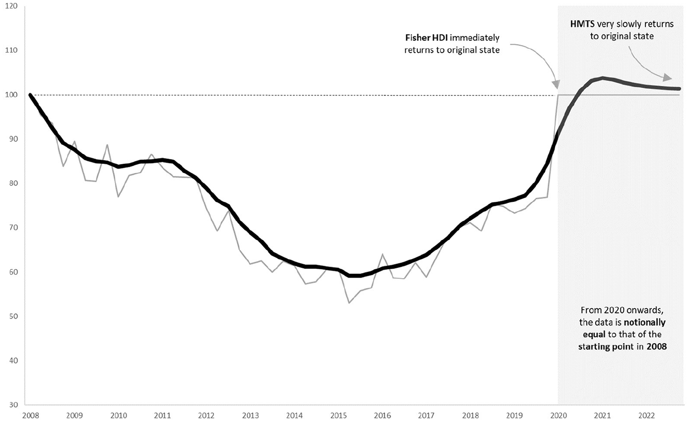
The identity test.

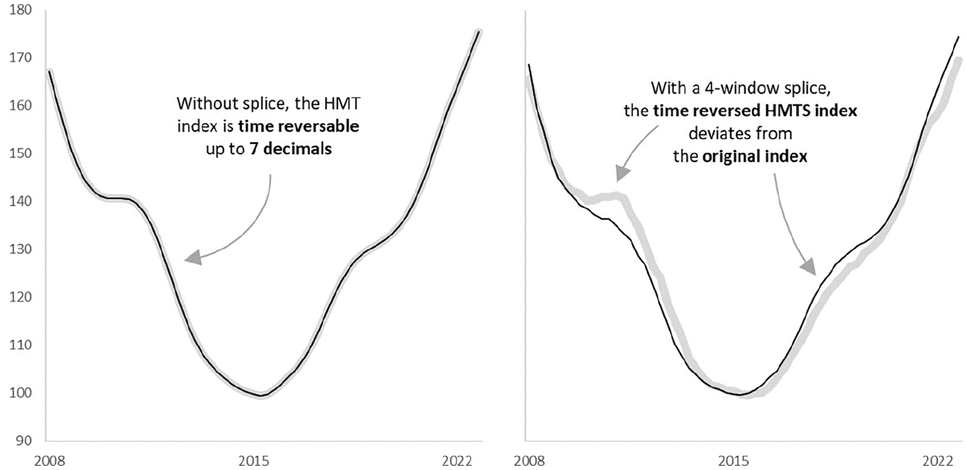
The time reversal test states that the price index of period A relative to B should be the opposite of the price index of period B relative to A. Since the prices are re-estimated with help of the entire series, time reversibility can’t be proven mathematically. Figure 8, therefore, shows an empirical test. A version of the index is calculated where all periods are reversed. The resulting index is then reversed again and the figures are compared to the original index. The figure shows that the indices without splice resemble the original index. In numbers, the indices are fully alike up to seven decimals for the entire index series. Adding the splice, violates the time reversibility. This was expected as the splices of the time reversed index, are shifted and contain (slightly) different information. The consequence is that the HMTS index is not fully independent of a base period. It does rely on the events to occur in one chronological order (and luckily, they do). In terms of index properties, this is a disadvantage, but like the identity test, this is a sacrifice that is likely worth it (given all benefits discussed Subsection 2.2).

Figure 8.

The time reversal test: reference year 2015.

The circular test states that the results between three periods should be consistent: multiplying the index between A and B with the index between B and C should be equal to the direct index between A and C. Circularity is introduced in the multilateral imputations step, but after the re-estimation and the window splice, the index loses this characteristic. Figure 9 shows an empirical test: indices are calculated with different starting points: 2008, 2009, 2010, and 2011. If circular, the indices should exactly overlap. The figure shows, however, that the indices do not overlap and thus the index is not circular. However, it also shows that the effect of using different base periods is minimal. This indicates that a certain level of circularity is retained. The indices differ the most at the start of the series. This is because the HMTS uses information of adjacent periods. As the series start in later periods, information is missing. Soon after the start of the series, the index levels and developments are quite similar.

Figure 9.

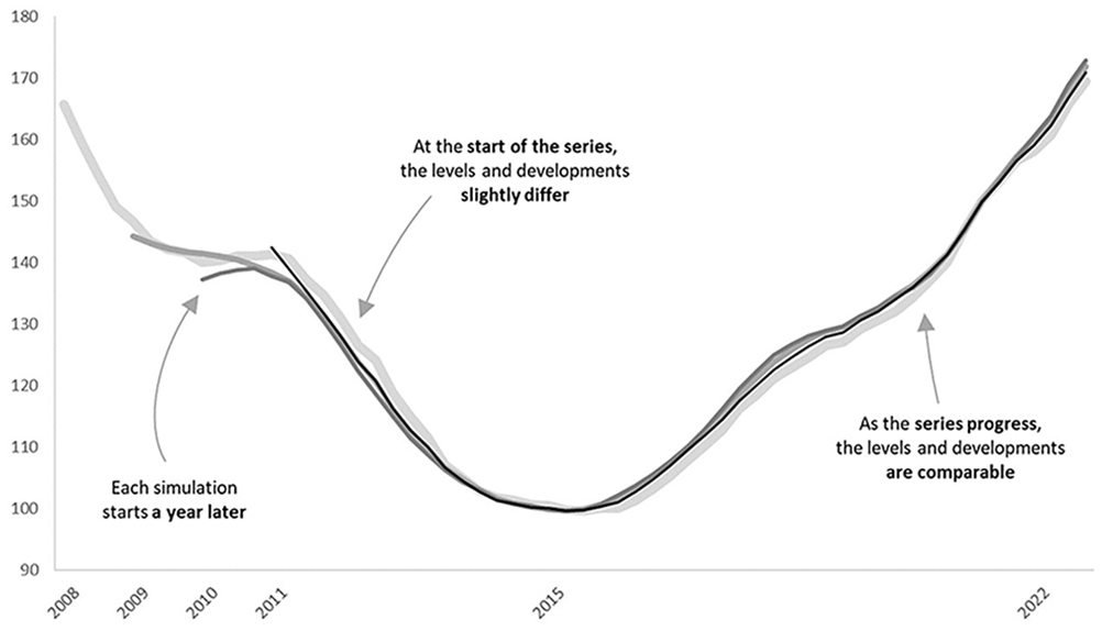
Circularity test: reference year 2015.

4.5. Reference Comparisons

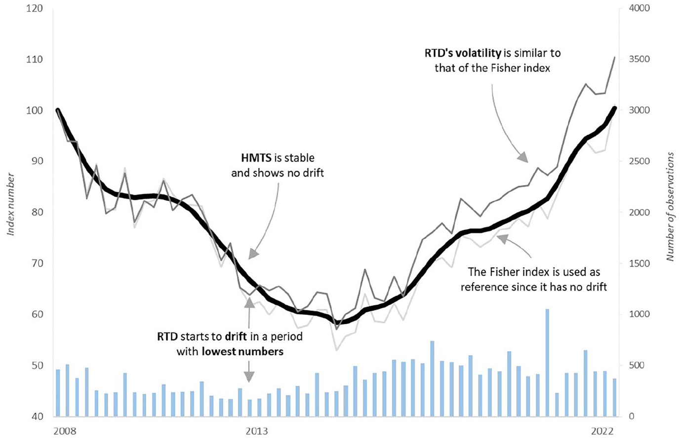
The Rolling Time Dummy (RTD) method (De Haan 2015; Hill et al. 2022) is one of the most serious alternatives when it comes to small domains and heterogeneous markets. The multiperiod regression increases the sample size (thus lowering the effect of small domains with heterogeneous markets) and the rolling window prevents continues revisions. Figure 10 shows the HMTS index alongside the RTD index and the Fisher HDI index. The RTD is calculated with a window length of three periods and a movement splice as described by De Haan (2015). The RTD index still shows volatility similar to the Fisher HDI index. In addition, the RTD shows drift, caused by “weak” periods in 2013. The Fisher index has no drift (by definition) and, therefore, illustrates the impact of the RTD’s drift. The RTD was also calculated with increased window lengths. Each window-increase caused the index to be closer to the Fisher index. This proves the sensitivity of the RTD to drift. The HMTS index is stable and shows no sensitivity to drift.

Figure 10.

HMTS, Fisher HDI, and Three-Window Rolling Time Dummy (RTD).

As time series re-estimation is introduced in step 3 of the method, there may be a concern for delay in the HMTS index. By looking at Figure 10, there is no solid way to tell if the HMTS lags the Fisher index. A test for Granger causality as used by Shimizu et al. (2010) is also performed in this study to investigate lead-lag relationships. The tests were run pairwise on the HMTS and a hedonic double imputation index with the first period as base period (step 1), a multilateral hedonic double imputation index (step 2) and Fisher hedonic double imputation index. Both a possible lead and lag role for the HMTS was tested. With p-values of respectively 1.371 × 10⁻⁴, 5.827 × 10⁻⁴, and 1.657 × 10⁻⁰⁶, a lag role of the HMTS is in all cases significant. However, with p-values of respectively 3.154 × 10⁻¹³, 5.127 × 10⁻¹⁶, and 1.678 × 10⁻¹², this shows that there is no clear lag of the HMTS. If any, the HMTS leads the other indices, most likely due to minimal volatility: a Fisher peak is, for example, a rise followed by a drop. If there was a downward trend before, the HMTS probably shows a drop twice and thus leads the Fisher index.

5. Conclusion

The HMTS index shows several practical advantages. There is an option to reduce and lengthen the number of provisional periods. Furthermore, stability is introduced without losing market information like a timely detection of turning points. It also reduces the reliance on the base period. This can be beneficial in case of insecurities about data quality or representativeness. Regarding CRE, this is often the case. The methodological index tests on the other hand, are not strictly (mathematically) met by the HMTS method. Analyses show, however, that the time reversal test is approximately (numerically) met in practice without splice. The splice creates a loss of time reversibility. This property of the HMTS shows that a sequential order of time is important. It is, however, good to see that right before slicing, time reversibility is mostly retained. The circular test is not fully met in practice, but analyses show that a large amount of circularity is retained in the index construction. Independence of one base period is especially important in small domains and the result in the circularity test shows the effectiveness of the HMTS in this regard. The identity test is not mathematically nor numerically met. Certainly, in cases of small domains with heterogeneous observations, the identity property may not be the index characteristic to primarily aim for. As shown in the analyses, identity-proof indices directly reflect changes in prices, regardless of the trend. If an index level is at 150 and the prices indicate a drop by 50%, an index that meets the identity test returns to 100 immediately. This is exactly what makes an index volatile. The assumption in the HMTS method is that the observations are subject to transaction noise. The lower the transaction numbers and higher the degree of heterogeneity, the safer this assumption seems to be. All in all, the methodological properties are not mathematically met, but in cases of small domains and heterogeneous markets (such as in commercial real estate) it may be worthwhile to loosen the desirability of these properties and balance it with practical properties.

The HMTS index is constructed with the desired properties of statistical agencies in mind. As the results seem adequate and the index outperforms the alternatives at some critical points, the HMTS index may aid statistical agencies in constructing reliable CPPIs. Complexity of the method and many hours of required coding can be considered disadvantages of the method. The code in R programming language is, therefore, available at request from the authors.

The HMTS could be applied beyond commercial real estate. A next best application would be for the construction of house price indices at a lower regional level, which can also be small domains. This relates to the strategic goals of statistical agencies and user’s needs to measure phenomena at a more regional level. As long as a hedonic model is used, the HMTS is applicable. Beyond real estate, however, it has not been studied. This is a topic for future study. A remark on using the HMTS method, is that if a common index method is sufficient, this probably has the preference. Primarily in case of small domains and heterogeneous goods, and when common index methods fail at capturing realistic price developments, the HMTS may provide a solid alternative.

5.1. Research Limitations

In cases where there are (almost) no observations, the HMTS index in its current form does not work. Each period should have a few observations with explanatory variables that show variation. A possibility to solve this, is to implement a multiperiod regression in the hedonic imputation: if a period does not have sufficient observations, the observations of the adjacent periods are added to complete the regression. This possibility has not been fully studied yet.

Footnotes

Appendix

Appendix 2.

Results Time Series Analyses.

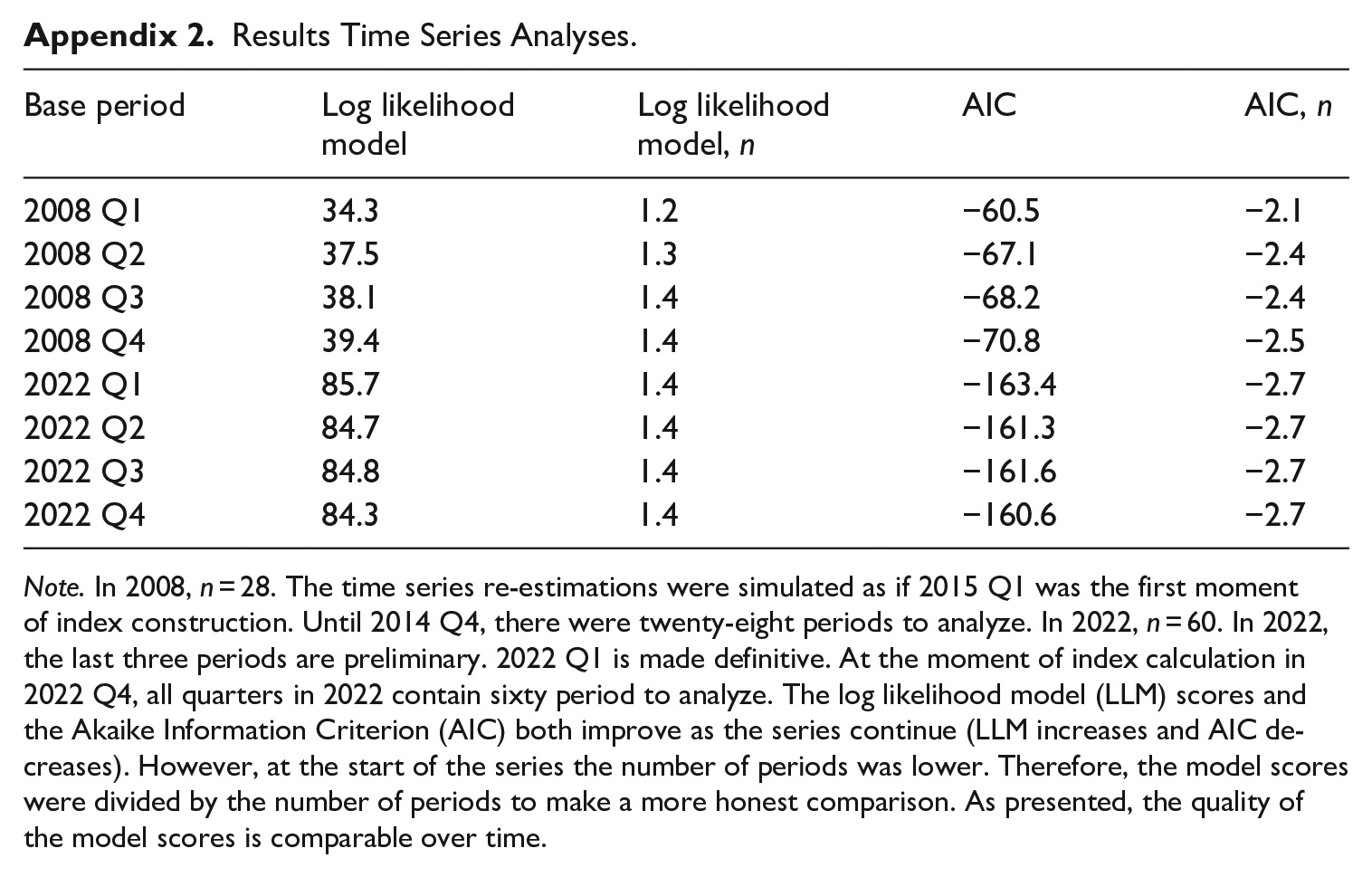
Base period	Log likelihood model	Log likelihood model, n	AIC	AIC, n
2008 Q1	34.3	1.2	−60.5	−2.1
2008 Q2	37.5	1.3	−67.1	−2.4
2008 Q3	38.1	1.4	−68.2	−2.4
2008 Q4	39.4	1.4	−70.8	−2.5
2022 Q1	85.7	1.4	−163.4	−2.7
2022 Q2	84.7	1.4	−161.3	−2.7
2022 Q3	84.8	1.4	−161.6	−2.7
2022 Q4	84.3	1.4	−160.6	−2.7

Note. In 2008, n = 28. The time series re-estimations were simulated as if 2015 Q1 was the first moment of index construction. Until 2014 Q4, there were twenty-eight periods to analyze. In 2022, n = 60. In 2022, the last three periods are preliminary. 2022 Q1 is made definitive. At the moment of index calculation in 2022 Q4, all quarters in 2022 contain sixty period to analyze. The log likelihood model (LLM) scores and the Akaike Information Criterion (AIC) both improve as the series continue (LLM increases and AIC decreases). However, at the start of the series the number of periods was lower. Therefore, the model scores were divided by the number of periods to make a more honest comparison. As presented, the quality of the model scores is comparable over time.

Acknowledgements

The authors would like to thank Peter Boelhouwer, Jan de Haan, Miriam Steurer, Robert Hill, and Norbert Pfeifer for reviewing draft versions of the paper and providing valuable feedback.

Funding

The author(s) declared that they received no financial support for the research, authorship, and/or publication of this article.

Received: March 2023

Accepted: May 2024

References

Babbie

Earl R.

2014. The Practice of Social Research. 10th ed. Belmont: Wadsworth/Thomson Learning.

Balk

Bert M.

1995. “Axiomatic Price Index Theory: A Survey.” International Statistical Review 63 (1): 69–93. DOI: https://doi.org/10.2307/1403778.

Balk

Bert M.

2012. Price and Quantity Index Numbers: Models for Measuring Aggregate Change and Difference. Cambridge: Cambridge University Press. https://books.google.nl/books?hl=nl&lr&id=ZvSkHKo1iZMC&oi=fnd&pg=PR11&dq=index+axiom+balk&ots=ghCSQBpo4F&sig=9Dlc.

Bentley

Alan

. 2022. “Rentals for Housing: A Property Fixed-Effects Estimator of Inflation from Administrative Data.” Journal of Official Statistics 38 (1): 187–211. DOI: https://doi.org/10.2478/jos-2022-0009.

CBS. 2022. “Measuring Commercial Property Prices.” https://www.cbs.nl/en-gb/about-us/innovation/project/measuring-commercial-property-prices.

Chessa

Antonio G.

2021. “Extension of Multilateral Index Series Over Time: Analysis and Comparison of Methods.” In 2021 Meeting of the Group of Experts on Consumer Price Indices, edited by Chessa

Antonio G.

The Hague: Statistics Netherlands.

Clapham

Eric

Englund

Peter

Quigley

John M.

Redfearn

Christian L.

2006. “Revisiting the Past and Settling the Score: Index Revision for House Price Derivatives.” Real Estate Economics 2 (34): 275–302. DOI: https://doi.org/10.1111/j.1540-6229.2006.00167.

Commandeur

Jacques J. F.

Koopman

Siem Jan

. 2007. An Introduction to State Space Time Series Analysis. Oxford: Oxford University Press.

De Haan

Jan

. 2015. “Rolling Year Time Dummy Indexes and the Choice of Splicing Method.” In Room Document at the 14th Meeting of the Ottawa Group, May (Vol. 22). https://www.stat.go.jp/english/info/meetings/og2015/pdf/t1s3room.pdf.

10.

De Haan

Jan

Van der Grient

Heymerik A.

2011. “Eliminating Chain Drift in Price Indexes Based on Scanner Data.” Journal of Econometrics 161 (1): 36–46. DOI: https://doi.org/10.1016/j.jeconom.2010.09.004.

11.

De Haan

Jan

Van der Grient

Heymerik

. 2008. “Indexcijfers.” Den Haag/Heerlen. www.cbs.nl.

12.

Deng

Yongheng

Quigley

John M.

2008. “Index Revision, House Price Risk, and the Market for House Price Derivatives.” Journal of Real Estate Finance and Economics 37 (3): 191–209. DOI: https://doi.org/10.1007/s11146-008-9113-7.

13.

Diewert

W. Erwin

. 2007. “Index Numbers.” Discussion Paper 07-02, Department of Economics.

14.

Diewert

W. Erwin

. 2020. “Basic Index Number Theory.” Discussion Paper 20-02, Vancouver School of Economics.

15.

Diewert

W. Erwin

Fox

Kevin J.

2022. “Substitution Bias in Multilateral Methods for CPI Construction.” Journal of Business and Economic Statistics 40 (1): 355–69. DOI: https://doi.org/10.1080/07350015.2020.1816176.

16.

Durbin

Koopman

S. J.

2012. Time Series Analysis by State Space Methods. 2nd ed. Oxford: Oxford University Press. http://www.oup.co.uk/academic/science/maths/series/osss/.

17.

Efron

Bradley

Tibshirani

Robert

. 1994. An Introduction to the Bootstrap. New York, NY: Chapman & Hall.

18.

Eichhorn

1976. “Fisher’s Tests Revisited.” Econometrica 44 (2): 247–56.

19.

European Commission. 2021. “Progress Report on Commercial Real Estate Statistics.” Brussels. https://ec.europa.eu/eurostat/documents/7590317/14115047/SWD-2021-421-Commercial-real-estate-statistics.pdf.

20.

European Union. 2023. “Commission Implementing Regulation (EU) 2023/1470.” Brussels. https://eur-lex.europa.eu/eli/reg_impl/2023/1470/oj.

21.

Eurostat. 2013a. ESS Guidelines on Revision Policy for PEEIs. Luxembourg: Publications Office of the European Union.

22.

Eurostat. 2013b. Handbook on Residential Property Prices (RPPIs). Luxembourg: Publications Office of the European Union. https://doi.org/10.5089/9789279259845.069.

23.

Eurostat. 2017. “Commercial Property Price Indicators: Sources, Methods and Issues.” Eurostat Methodologies & Working Papers. Publications Office of the European Union. https://doi.org/10.2785/050176.

24.

Eurostat. 2022. Guide on Multilateral Methods in the Harmonised Index of Consumer Prices. Luxembourg: Publications Office of the European Union.

25.

Francke

Marc K.

2010. “Repeat Sales Index for Thin Markets.” Journal of Real Estate Finance and Economics 41 (1): 24–52. DOI: https://doi.org/10.1007/s11146-009-9203-1.

26.

Francke

Marc K.

de Vos.

A. F.

2000. “Efficient Computation of Hierarchical Trends.” Journal of Business & Economic Statistics 18 (1): 51–7. DOI: https://doi.org/10.1080/07350015.2000.10524847.

27.

FSB, and IMF. 2022. “G20 Data Gaps Initiative (DGI-2) Progress Achieved, Lessons Learned, and the Way Forward.” https://www.fsb.org/2022/06/g20-data-gaps-initiative-dgi-2-progress-achieved-lessons-learned-and-the-way-forward/.

28.

Hill

Robert J.

Rambaldi

Alicia N.

Scholz

Michael

. 2021. “Higher Frequency Hedonic Property Price Indices: A State-Space Approach.” Empirical Economics 61 (1): 417–41. DOI: https://doi.org/10.1007/s00181-020-01862-y.

29.

Hill

Robert J.

Scholz

Michael

Shimizu

Chihiro

Steurer

Miriam

. 2022. “Rolling-Time-Dummy House Price Indexes: Window Length, Linking and Options for Dealing with Low Transaction Volume.” Journal of Official Statistics 38 (1): 127–51. DOI: https://doi.org/10.2478/jos-2022-0007.

30.

Hill

Robert J.

Steurer

Miriam

. 2020. “Commercial Property Price Indices and Indicators: Review and Discussion of Issues Raised in the CPPI Statistical Report of Eurostat (2017).” Review of Income and Wealth 66 (3): 736–51. DOI: https://doi.org/10.1111/roiw.12473.

31.

ILO, International Monetary Fund, Eurostat, United Nations Economic Commission for Europe, Organisation for Economic Co-operation and Development, and The World Bank. 2020. “Consumer Price Index Manual, Concepts and Methods.”

Washington, D.C.

www.elibrary.imf.org.

32.

Ivancic

Lorraine

Diewert

W. Erwin

Fox

Kevin J.

2011. “Scanner Data, Time Aggregation and the Construction of Price Indexes.” Journal of Econometrics 161 (1): 24–35. DOI: https://doi.org/10.1016/j.jeconom.2010.09.003.

33.

Johnson

R. W.

2001. “An Introduction to the Bootstrap.” Teaching Statistics 23 (2): 49–54. http://danida.vnu.edu.vn/cpis/files/Refs/LAD/An Introduction to the Bootstrap.pdf.

34.

Kalman

R. E.

1960. “A New Approach to Linear Filtering and Prediction Problems.” Journal of Basic Engineering 82: 35–45. DOI: https://doi.org/10.1115/1.3662552.

35.

Krsinich

Frances

. 2016. “The FEWS Index: Fixed Effects with a Window Splice.” Journal of Official Statistics 32 (2): 375–404. DOI: https://doi.org/10.1515/JOS-2016-0021.

36.

Miyakawa

Daisuke

Shimizu

Chihiro

Uesugi

Iichiro

. 2024. “Do Foreign Buyers Pay More Than Domestic Buyers? Evidence from International Transaction-Level Data.” The Journal of Real Estate Finance and Economics 68: 394–424. DOI: https://doi.org/10.1007/s11146-022-09937-6.

37.

OECD. 2012. “Quality Framework and Guidelines for OECD Statistical Activities.” https://www.oecd.org/sdd/qualityframeworkforoecdstatisticalactivities.htm.

38.

O’Hanlon

Niall

. 2011. “Constructing a National House Price Index for Ireland.” Journal of the Statistical and Social Inquiry Society of Ireland 40: 167–96. Available at: http://hdl.handle.net/2262/62349.

39.

Pierson

N. G.

1896. “Further Considerations on Index-Numbers.” The Economic Journal 6 (21): 127–31. Available at: https://about.jstor.org/terms.

40.

Rambaldi

Alicia N.

Fletcher

Cameron S.

2014. “Hedonic Imputed Property Price Indexes: The Effects of Econometric Modeling Choices.” Review of Income and Wealth 60 (S2): S423–48. DOI: https://doi.org/10.1111/roiw.12143.

41.

Schwann

Gregory M.

1998. “A Real Estate Price Index for Thin Markets.” Journal of Real Estate Finance and Economics 16 (3): 269–87.

42.

Shimizu

Chihiro

Nishimura

Kiyohiko G.

Watanabe

Tsutomu

. 2010. “Housing Prices in Tokyo: A Comparison of Hedonic and Repeat Sales Measures.” Jahrbücher für Nationalökonomie und Statistik 230 (6): 792–813. DOI: https://doi.org/10.1515/jbnst-2010-0612.

43.

Silver

Mick

. 2016. “How to Better Measure Hedonic Residential Property Price Indexes.” IMF Working Papers. Vol. 16. DOI: https://doi.org/10.5089/9781475552249.001.

44.

UN. 2014. “Fundamental Principles of Official Statistics.” Sixty-Eighth Session of General Assembly. Vol. 9. https://unstats.un.org/unsd/dnss/gp/fundprinciples.aspx.

45.

Wald

1937. “Zur Theorie Der Preisindexziffern.” Journal of Economics 8 (2): 179–219. https://about.jstor.org/terms.

46.

Willenborg

Leon

. 2017. From GEKS to Cycle Method. The Hague: Statistics Netherlands.

47.

Willenborg

Leon

. 2018. Transitivity of Price Indices. The Hague: Statistics Netherlands.

48.

Willenborg

Leon

Scholtus

Sander

. 2018. Bootstrapping the SPAR Index. The Hague: Statistics Netherlands. DOI: https://doi.org/10.13140/RG.2.2.22772.60802.

Constructing Limited-Revisable and Stable CPPIs for Small Domains

Abstract

Keywords

1. Introduction

2. Background

2.1. Desired Methodological Properties

2.2. Desired Practical Properties

3. Methodology

3.1. Step 1: Hedonic Imputations

3.2. Step 2: Multilateral Imputations

3.3. Step 3: Time Series Re-Estimated Imputations

3.4. Step 4: Window Splice

4. Data and Empirical Findings

4.1. Data: Office Building Transactions in the Netherlands

4.2. Results Step 1 to 4

4.3. Assessment of Practical Properties

4.4. Assessment of Methodological Properties

4.5. Reference Comparisons

5. Conclusion

5.1. Research Limitations

Footnotes

Appendix

Acknowledgements

Funding

References