
Abstract
Relational event models (REMs) are the primary choice for the analysis of relational-event network data. However, the standard REM assumes static parameters, which hinders the modeling of time-varying dynamics. This assumption might be too restrictive in real-life scenarios, making a model that allows for time-varying parameters more valuable. We introduce a state-space extension of the relational event model as a way to tackle this problem. The model has three main attributes. First, it provides a statistical framework of the temporal change of the parameters. Second, it enables the forecasting of future parameter values (which can be utilized to simulate new networks that can account for temporal dynamics in out-of-sample predictions). Third, it requires smaller data structures to be loaded into computer memory compared to the standard REM; this makes the model easily scalable to large networks. We conduct empirical analyses on bike-sharing data, corporate communications, and interactions among socio-political actors to illustrate model usage and applicability.
Introduction
Relational event data are a representation of a social network data that contain information on actors’ interactions over time (Butts and Marcum, 2017) by encoding who interacts with whom at what point in time. This data type can provide a wealth of insights for social science researchers interested in unveiling the intricacies of social interactions. With the advent of new technologies, such as web applications that allow for instant messaging, these data have become increasingly prevalent. Research analyzing relational event data has appeared in a variety of disciplines and topics, ranging from logistics (Vu et al., 2017) to finance (Zappa and Vu, 2021), and from social hierarchies (Redhead and Power, 2022) to friendships (Goodreau et al., 2009; Meijerink-Bosman et al., 2023).
The relational event model (REM) introduced by Butts (2008) is the stepping stone of most of the research published in this field. This model has been extended in many different ways. Perry and Wolfe (2013) have proposed a partial likelihood approach for modeling the receiver given the sender. Extensions have been proposed to model the memory decay of past interactions (Arena et al., 2023a). Karimova et al. (2023) applied regularization methods to perform variable selection in relational event models.
The relational event model is dynamic in the sense that its log-linear regression structure allows the introduction of time-varying covariates. This allows the rate at which specific network interactions occur to vary over time. However, the REM does not allow the regression parameters themselves to vary over time, which might be a restrictive assumption, given the dynamic nature of relational event data. Although the REM allows for the rate of dyadic interactions to be different at different points in time, the exact way in which it depends on previous interactions is assumed to remain constant. In real-life social interaction data the interaction rate between actors can be highly dynamic (Boschee et al., 2015; Klimt and Yang, 2004; O’Mahony and Shmoys, 2015) and the way in which actors respond to different levels of transitivity or subgroup membership can change over time. Social network researchers are interested in understanding what drives these dynamics. For example, it could be the case that the average event rate (captured by the intercept) changes over time, while the effects of social interaction structure (e.g. inertia, reciprocity, participation shifts) remain roughly constant. Conversely, it could also be that the intercept remains constant and structural interaction mechanisms time-vary. Either way, it may often be desirable to allow the values of the parameters in the relational event model to vary over time, rather than only the values of the (exogenous and endogenous) statistics.
In this paper, we propose a state-space model for relational event data. The state-space model is the gold standard for dynamic modeling (West et al., 1985; West and Harrison, 1989, 2006), but it has not been applied in the relational event model literature. In traditional state-space models, the parameters change after every observation (Petris et al., 2009). However, this is not realistic within the REM framework. First, a single event says very little about the global network dynamics. Second, the REM uses sufficient statistics in its specification. These are computed as functions of past events, and having only a single event precludes the computation of most network statistics. In order to obtain insight into real-world network dynamics, it often suffices to understand how the parameters change on a slightly wider temporal scale. Thus, to take this into account, we split the event sequence into blocks of meaningful time units (e.g. seconds, minutes, hours) and assume the parameters to be fixed throughout that specific period only. Then, we assume a state-space model for these relational event sequence blocks.
This model has the following properties: (i) it provides a formal framework to model the dynamics governing the time-varying parameters; (ii) it allows for the estimation of parameters for future time points (this can be used to simulate future networks that takes temporal dynamics into account in out-of-sample predictions); (iii) by separating the relational event sequence in blocks, only a smaller portion of the data matrix needs to be loaded into computer memory, which makes the model much more scalable to large networks than the traditional REM. Other approaches have also been proposed for time-varying REM parameters (e.g. Kamalabad et al., 2023; Mulder and Leenders, 2019; Vu et al., 2011) but they do not possess the same attractive properties as the state-space model. To illustrate the model, we conduct empirical analyses on bike sharing in New York City (O’Mahony and Shmoys, 2015), corporate email communications (Klimt and Yang, 2004), and interactions among socio-political actors in India (Boschee et al., 2015).
The remainder of the text is structured as follows: Section 2 briefly describes the relational event model; Section 3 presents the state-space model and describes algorithms used for model estimation and prediction; Section 4 features the application of the proposed model to three different empirical data sets; and Section 5 concludes the paper with a discussion of the main points and offers future research routes.
The relational event model
A relational event sequence is defined as an ordered sequence of dyadic events among a finite set of actors along a time scale (Butts and Marcum, 2017). In its simplest form, a dyadic event entails a sender of an interaction, a receiver, and the time point at which the interaction occurred. Thus, let a network contain
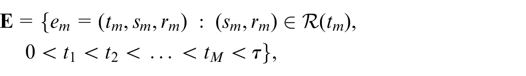
where
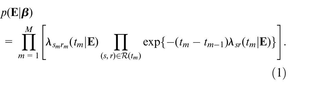
Butts (2008) assumes a constant piecewise exponential model for these data (Friedman, 1982), where the rate of events between actors
The likelihood function of this model is given by
In this paper, we will write
A state space approach for the relational event model
In traditional state-space models, the parameters change after every observation (Petris et al., 2009). Thus, assuming a state-space model for the relational event sequence, for every event
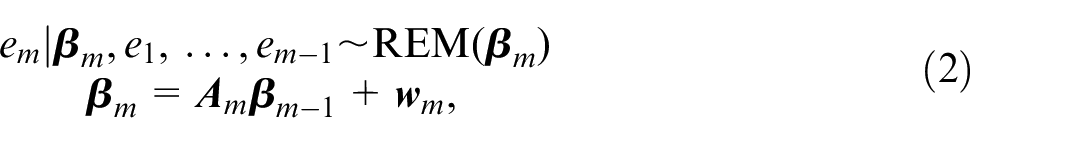
where
Generally, in relational event modeling, the interest is in fairly broad temporal dynamics that are unlikely to be captured by changing the parameters after every event. For instance, Mulder and Leenders (2019) considered relational event data of email exchanges among colleagues in a company’s department. They were interested in analyzing how the information-sharing behavior changes over a period of several months. Thus, they analyzed the temporal changes on monthly intervals, even though the timing of the emails themselves is much more fine-grained (in their dataset milliseconds).
In this study, we consider the case where it can be assumed that the effects represented by
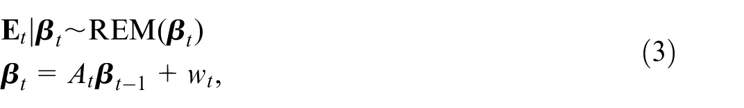
where
Vieira et al. (2023) have shown that a REM can be approximated by a Gaussian distribution in case the size of the batch
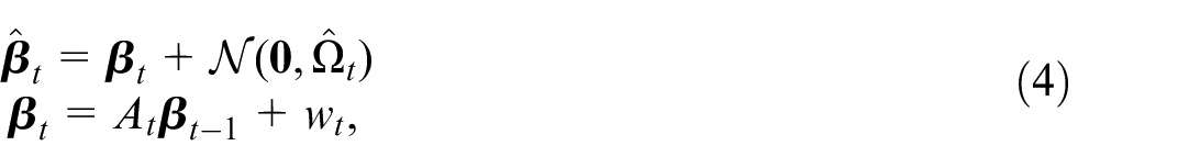
where
Computationally, one of the main advantages of the setup in equation (4) is that it saves considerable amounts of computer memory. For the static REM, the data matrix
In summary, the main idea of the state-space model is that for every discrete time point, there exists an underlying temporal process in nature (e.g. the natural conditions through which actors interact between themselves), which we call the state process
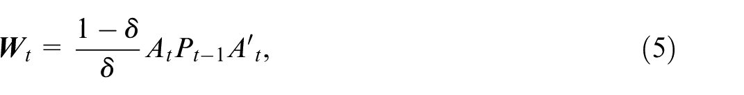
Weight matrix specification
The matrix
The state process innovation covariance matrix
From equation (4), it is clear that the residual covariance matrix of the state process equation
First, note that the residual state process covariance matrix is responsible for balancing the passing of information from

If there is no error in the estimation of the state
where
Model estimation: The Kalman filter
The Kalman filter is an iterative procedure used for parameter estimation and prediction (Kalman, 1960; Kalman and Bucy, 1961). This algorithm leverages the Gaussian structure of the model in equation (4). The steps to estimate this model via the Kalman filter are given in Algorithm 1. The Kalman filter uses recursive estimation and prediction of the state of a dynamic system in the presence of noise. It operates recursively by updating its estimate of the state of the system as new measurements become available over time.
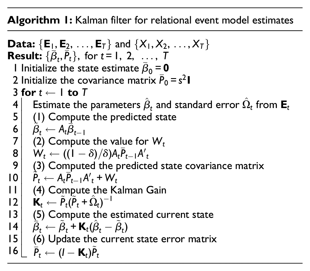
In the initial state
Predicting future events
One of the main advantages of the state-space model is that it provides a formal framework to predict future events while incorporating temporal dynamics. Algorithm 2 describes the steps to generate future events. This algorithm works by leveraging the state equation to generate predictions for future values of the network states. Subsequently, it generates new networks using that predicted stated as the true value for the parameters in the model.
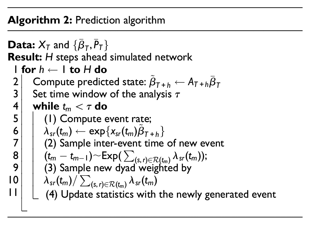
Here,
Finally, to generate prediction intervals, the covariance matrix of the newly predicted state
Empirical illustrations
In this Section, we provide three empirical examples to illustrate the model’s ability to capture time series relational event patterns. The goal is to show how the model can be used to study the temporal dynamics of social mechanisms and also to disentangle what explains the change in interaction rates in applications on bike sharing (O’Mahony and Shmoys, 2015), email communications (Klimt and Yang, 2004), and interactions among socio-political actors (Boschee et al., 2015). In all illustrations, we employed a discount factor of
Bike sharing in New York City
The sharing of Citi bikes in the city of New York is registered in this data set with timestamps, and start and end stations of each bike ride (O’Mahony and Shmoys, 2015).This data is freely available on https://citibikenyc.com/system-data. Table 1 shows the first five rows of the relational event sequence, the columns for sender and receiver represent the station where the ride started and the station where it ended, respectively. The data were analyzed hourly from 9 AM to 6 PM and represent the first 10 days of August 2023. The data have 111 stations and the 50 most active were selected. In total, 13,830 events were analyzed.
First five rows of the bike sharing data.
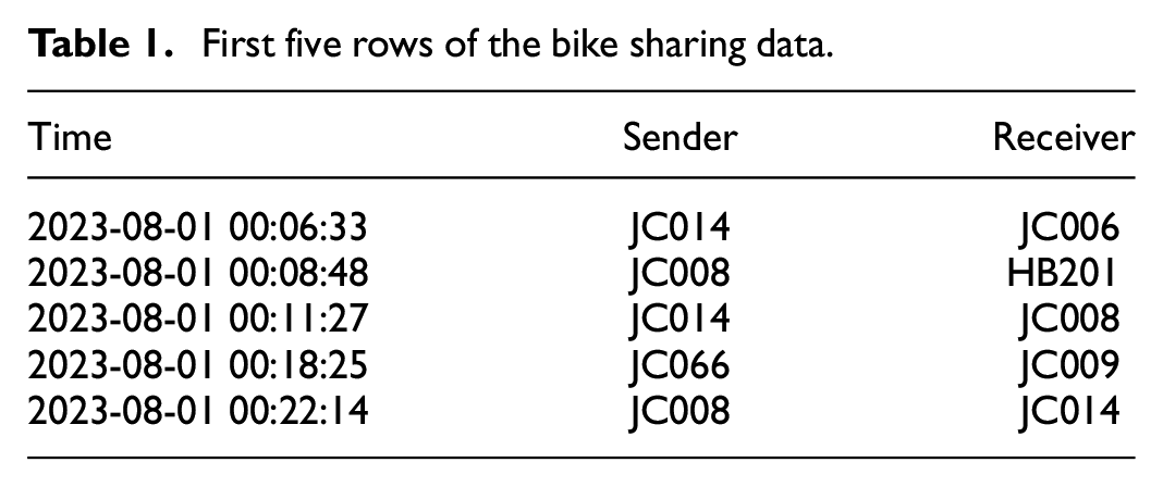
Figure 1 displays the number of events per hour, where every bar represents an hour. The time series displays strong seasonality with a spike in the number of events for the last 3 hours of the time window. The number of events per batch (i.e. per hour) ranges from a minimum of 31 to a maximum of 329 events. The number of dyads at risk at each point in time is 50 × 49 = 2450. Hence, the largest data matrix loaded into computer memory has dimensions 329 × 2450 × 5, as opposed to 13,830 × 2450 × 5 required by the static REM.
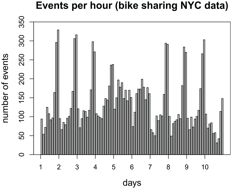
Number of events (bike rides) per hour from 9 AM to 6 PM for the first 10 days of August 2023.
We specified the rate of our model with an intercept and four network effects (out-degree sender, in-degree receiver, reciprocity, and inertia). The out-degree sender represents the number of bikes that started a ride at a certain station. The in-degree receiver is the number of bikes that finished a ride at a certain station. Reciprocity is the number of times that station A received a bike from station B, after sending a bike to station B. Inertia is the number of times that someone started a bike ride at station A and ended at station B. Thus, substantively, this model describes the bicycle traffic in terms of activity (out-degree) and popularity (in-degree) of stations. Moreover, inertia and reciprocity are also important in this context. For instance, if we think simply in terms of spatial distribution of stations, it is likely that commuters will use bicycles everyday to go from a station close to their homes to a station close to their work, accentuating the effect of inertia in the data. Then, they would take the inverse route to go back home, accentuating the effect of reciprocity.
Figure 2 shows the predicted state per hour in the first 10 days of August 2023. The shaded area is a
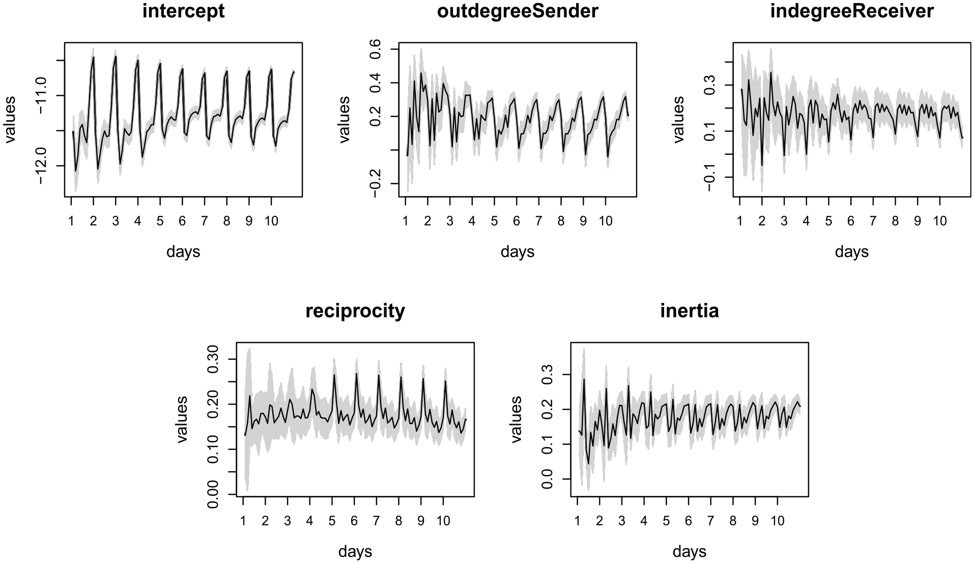
Predicted states per time point in the first 10 days of August 2023, for the bike sharing application.
Finally, Figure 3 displays a plot of the number of events with an out-of-sample prediction of one-day ahead, for the 10-day window analyzed. As it can be seen in Table 1, the events are recorded with a precision down to the seconds. Since we analyzed the relational event sequence in hourly intervals, we specified
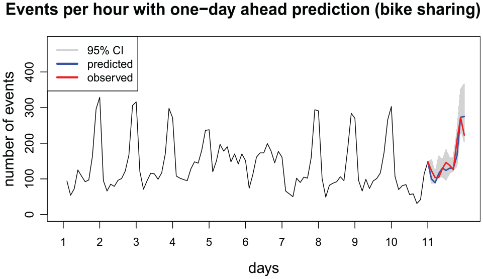
Number of events (bike rides) per hour from 9 AM to 6 PM for the first 10 days of August 2023 with predictions for the next day.
Predictions of number of events with 95% confidence interval and prediction error for the Bike sharing data.
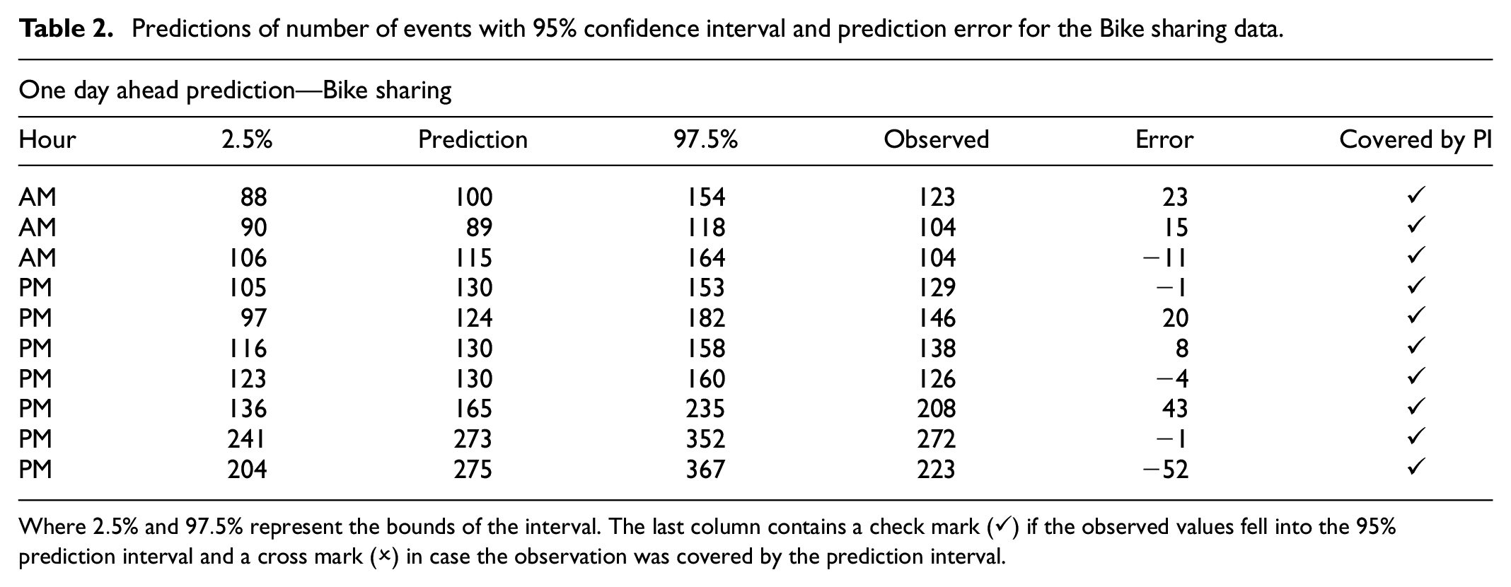
Where
Email communications in corporate networks
Enron was a company in the energy sector that went bankrupt after a series of events involving dubious accounting practices. The data set containing email communications among its employees has been featured in the literature in the past (Klimt and Yang, 2004; Perry and Wolfe, 2013). In this illustration, we follow Perry and Wolfe (2013) and analyze only those events that had five receivers or less. We consider the email data in the years of 2000 and 2001, this is the period in which the “Enron scandal” was unveiled. For instance, according to Bondarenko (2004), Enron’s share went from around $90 in the mid-2000 to less than $12 by the end of 2001. This time frame contains 153 actors and 34,180 events; we analyzed the events in monthly intervals. Our interest is in the general change of the email interaction structure over the 2-year period; intervals of 1 month results in batches with a sufficient number of events to use the Gaussian approximation approach (Vieira et al., 2023). The number of events in each batch ranges from 363 to 3403. Table 3 displays the first five rows in the relational event sequence.
First five rows of the Enron email data.
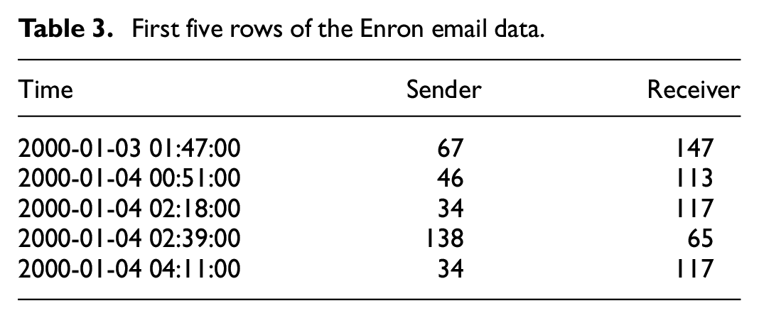
Figure 4 displays the number of events per month during the period analyzed, every bar represents 1 month. We can clearly see a growing trend in the number of emails across these 2 years. We specified a model with an intercept and six network effects (out-degree sender, in-degree sender, out-degree receiver, in-degree receiver, reciprocity, and inertia). The model captures the activity of senders and receivers through out-degree sender and out-degree receiver. It also includes the popularity of senders and receivers via in-degree sender and indegree-receiver. We included reciprocity to capture the tendency of email messages to be reciprocated and inertia to reflect the fact that usually in a company senders tend to mail the same receivers over and over (e.g. lower level employees reporting to managers via email).
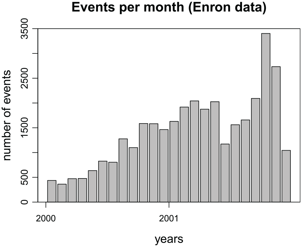
Number of events (emails) per month from January 2000 to December 2001.
Figure 5 presents the series of predicted states for this model, with shades representing
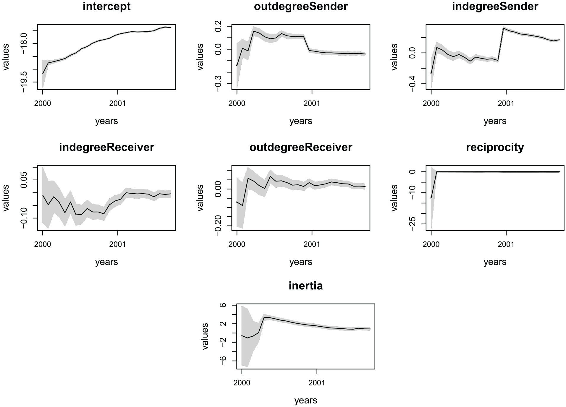
Predicted states per month from January 2000 to December 2001 for the Enron email data set.
Finally, as seen in Table 3 the events are recorded with timestamps down to the seconds. Thus, given that we analyzed events monthly, we specify
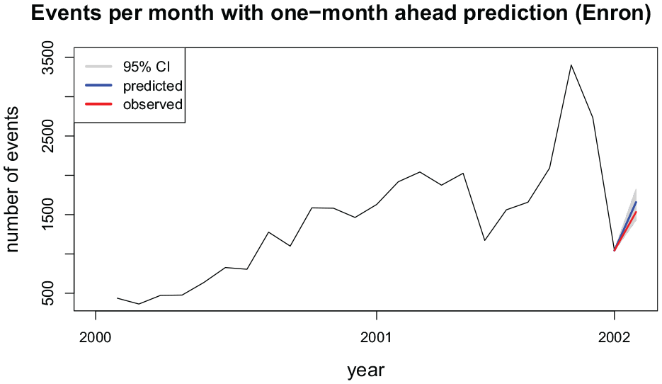
Number of events (emails) per month from January 2000 to December 2001 with a prediction for January 2002.
Predictions of number of events with 95% confidence interval and prediction error for the Enron email data.
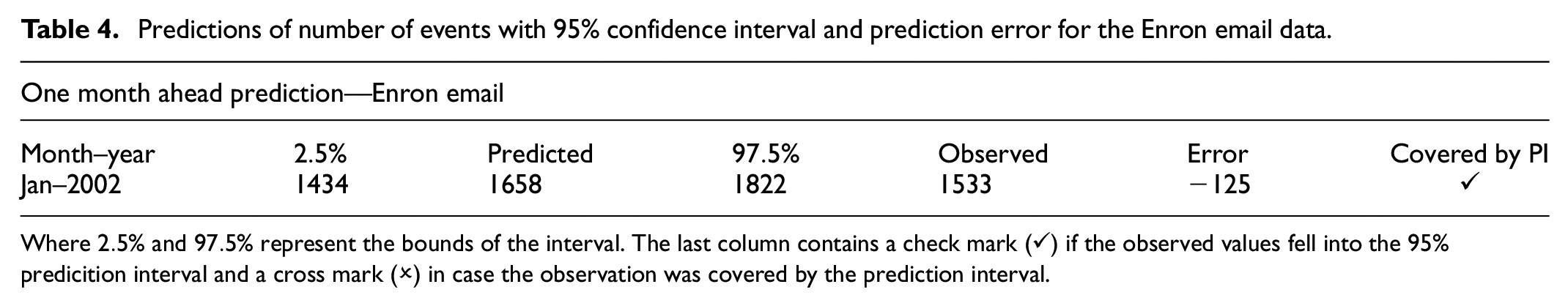
Where
Interactions between socio-political actors within news outlets
The Integrated Crisis Early Warning System (ICEWS) is a database consisting of dyadic interactions among socio-political actors collected from news outlets (Boschee et al., 2015).This system is used by the United States military to provide conflict early warnings that can help decision-makers to allocate resources and draw effective mitigation plans (O’brien, 2010). In this illustration, we analyze the network of monthly events among Indian socio-political actors from 2011 to 2018. The network contained a total of 1612 actors. Here, only the 50 most active actors were selected and in total, there were 419,274 events. Table 5 shows the first five rows of the relational event sequence. The number of events in each month ranges from 1397 to 8368.
First five rows of the ICEWS event history of interactions among Indian political actors.
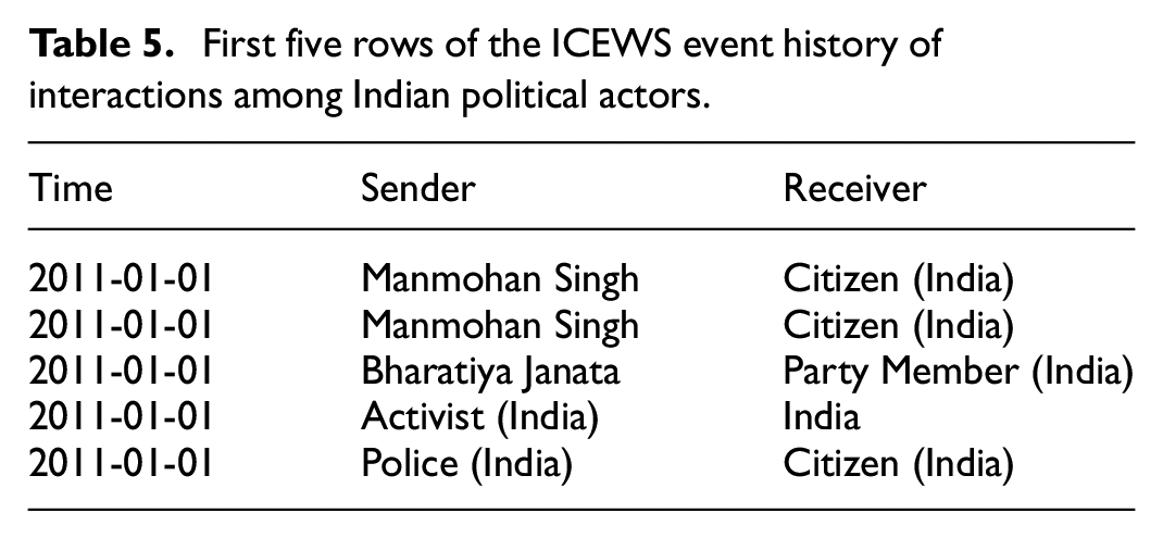
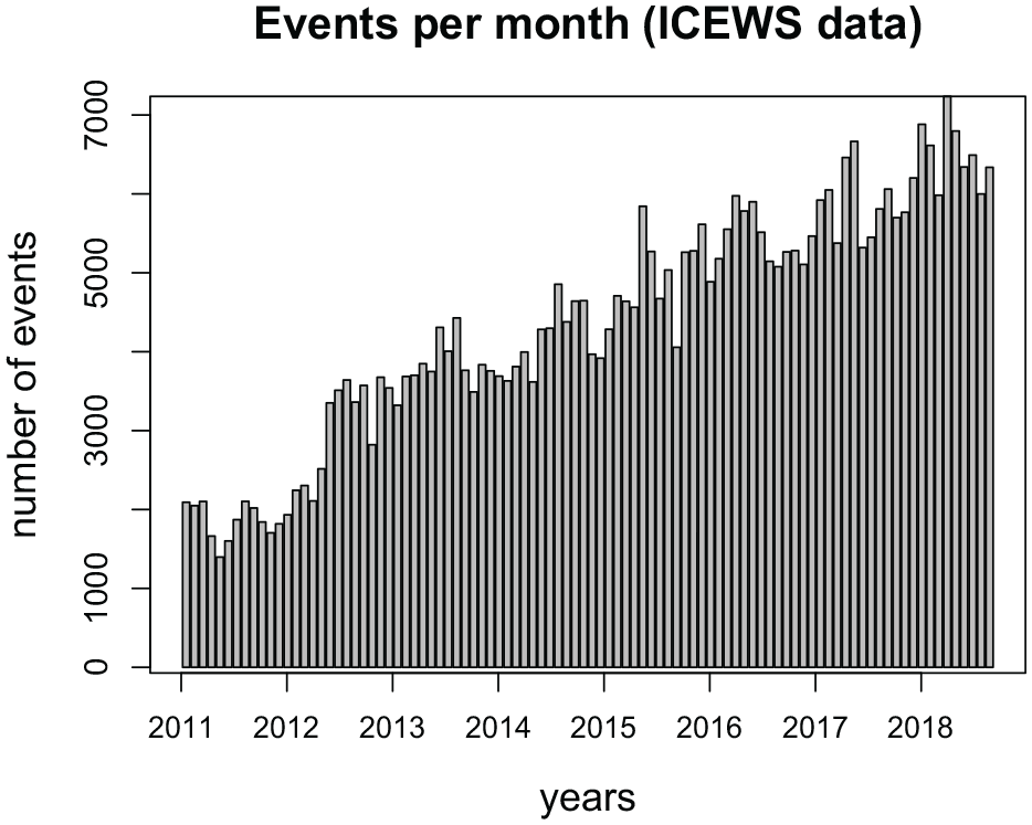
Figure 7 shows the distribution of the number of events from January 2011 to December 2018. These data display a strong upward trend and a very slight seasonality. We specify a model with an intercept and six network effects. We focus on analyzing the activity and popularity of senders and receivers by including the network effects out-degree sender (activity) and in-degree receiver (popularity). We also include inertia and reciprocity, to capture the tendency of actors to forge communications partnerships and reciprocate events, which can be important in the context of interactions amongst political entities. Finally, the participation shifts ABBA and ABXA were included in the model. The former indicates that after actor A sending an event to actor B, actor B immediately reciprocates (the difference between ABBA and reciprocity is that ABBA captures immediate reciprocation of the BA event by A, whereas reciprocity captures the tendency for A to respond to the accumulated past BA events). The latter indicates that after actor A sends an event to actor B, another actor X (different than B) sends an event to A. These participation shifts can be important in this context, given that politicians often refer to other politicians when addressing the press and giving speeches (Bhatia, 2006).
Number of events among Indian political actors extracted from news outlets per month from January 2011 to December 2018.
Figure 8 shows the predicted states for the effects in this model. The shaded areas are the 95% confidence intervals. As expected, the intercept presents a strong upward trend. A slight seasonality is clearly seen with the intercept, out-degree sender, and in-degree receiver, which indicates that these effects are mimicking the slight seasonality displayed in the series of number of events. The other effects display stationary behavior (except for inertia that displays a slight downward trend). Overall, the dynamics seem to be fairly stable for reciprocity, ABBA, and ABXA. Out-degree sender, in-degree receiver, and inertia display patterns that might point toward a future change in the level of these effects, with out- and in-degree being likely to increase slightly at the end of the observed time window and inertia being more likely to slightly decrease.
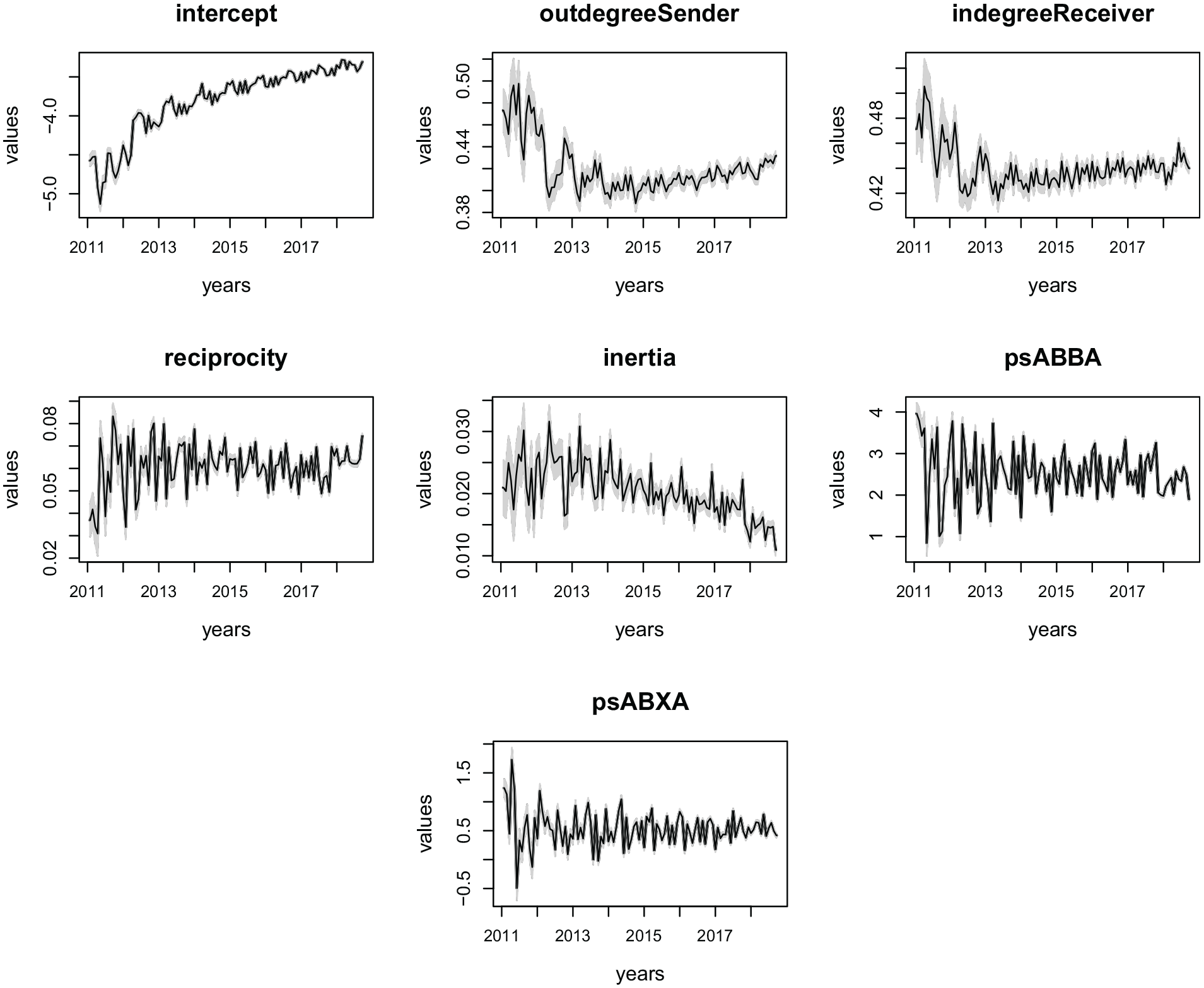
Predicted states per month from January 2011 to December 2018 for the ICEWS data set of interactions among Indian political actors.
Finally, Figure 9 shows the number of events with an out-of-sample prediction of 1-year-ahead for the year 2019. For these data, as opposed to the previous data sets presented, we do not have the timestamps of the events (see Table 5). All we know is the order in which the events occurred. This makes it hard to specify the
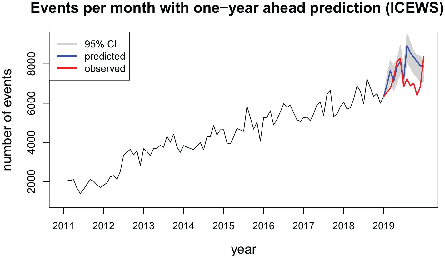
Number of events among Indian political actors extracted from news outlets per month from January 2011 to December 2018 with a prediction for the year 2019.
Hence, Figure 9 presents the predictions derived from
Predictions of number of events with 95% confidence interval and prediction error for the ICEWS data.
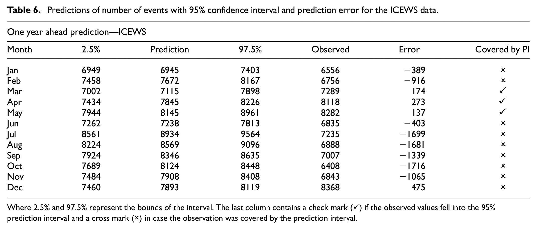
Where
Discussion
The relational event model (REM) has been the main choice in the literature for analyzing relational event data. However, even though this data type is essentially dynamic, the standard REM does not support the modeling of time-varying parameters. The static nature of the parameters in this model can be considered a restrictive assumption in most applications (see Section 4). This paper presented a state-space model extension of the relational event model. This model has three main advantages over the traditional REM. First, it is equipped with a formal rule that drives the parameter changes over time, being flexible enough to capture time series patterns (e.g. trend and seasonality) in the estimates without requiring additional modeling effort. This allow us to better understand what drives the changes in social interaction rates in the data. Second, it provides a framework to predict future states that can be used to produce out-of-sample predictions that take the temporal dynamics into account. Third, it requires smaller data structures making it more easily scalable to larger networks than the static REM. The use of these smaller structures is a big advantage, particularly for researchers who do not have vast computational resources at their disposal.
We presented three empirical illustrations to showcase the method. These applications concerned a varied set of data on bike sharing in New York City (O’Mahony and Shmoys, 2015), email communications in corporate networks (Klimt and Yang, 2004), and interactions between Indian socio-political actors in news outlets (Boschee et al., 2015).The examples show that it can be quite important to model the time-varying dynamics in relational event networks. If the static REM had been employed, we would have only learned average effects and miss the temporal information brought up by the state-space model.
On the other hand, there may be cases where the proposed state-space relational event model may not be preferred. One example would be when there are sudden changes in the interaction behavior between the actors which would cause abrupt changes of the model parameters. In this case, the state of the model parameters before the change could result in bad predictions right after the change, due to violations of the pre-specified values in the weight matrices
In this case, it may be preferred to estimate the weight matrix, even though this could be highly computationally intensive (see Section 3.1). State-space approaches for relational event models may also then be preferred (Kamalabad et al., 2023). Second, there might be rare instances where the interaction behavior is static in the sense that the model parameters remain approximately constant over the observational period. Using the state-space relational event model would then result in statistical overfitting where the noise could incorrectly be identified as the signal resulting in potential poor predictive performance. This may especially be the case when fitting relational event models with a very large number of possible drivers of social interaction behavior (Karimova et al., 2023).
We leave for future research the investigation of the choice of batch sizes. Most of the time, a researcher would be interested in a particular time unit (i.e. days, hours, weeks, etc.). In this case, the partition of the network is natural. However, it might be the case that partitioning according to a particular time unit might result in batches that are too small to use the Gaussian approximation. Thus, providing rules of thumb for the choice of batch sizes can aid researchers in deriving meaningful inferences from this model. Moreover, it is also useful to develop model evaluation metrics for the out-of-sample prediction. In the empirical illustrations we only predicted the future number of events (within a certain time period). For this purpose, metrics such as the root-mean-squared error (RMSE) would suffice for model evaluation. But, to obtain an estimate for the future number of events, multiple networks were generated. Therefore, there is a need to evaluate how well those simulated networks reflect the actual future observations. Although out-of-sample prediction has been used routinely to assess the fit of a relational event model, it is not yet clear how this would be used best in the case where model parameters change over time and the model might fit specific parts of the observation period better than other parts. Assessing model fit for dynamic models is a generally important issue and will need to be developed further in future research. Finally, another issue that needs to be tackled concerns the definition of the time window in which predictions will be generated, defined by
Footnotes
Declaration of conflicting interests
The author(s) declared no potential conflicts of interest with respect to the research, authorship, and/or publication of this article.
Funding
The author(s) disclosed receipt of the following financial support for the research, authorship, and/or publication of this article: This research was supported by the Netherlands Organization for Scientific Research (NWO) Grant to JM and FV (452-17-006).
Data availability statement
The data associated with the manuscript is available upon request.