
Abstract
Income inequality estimators are biased in small samples, leading generally to an underestimation. This aspect deserves particular attention when estimating inequality in small domains and performing small area estimation at the area level. We propose a bias correction framework for a large class of inequality measures comprising the Gini Index, the Generalized Entropy, and the Atkinson index families by accounting for complex survey designs. The proposed methodology does not require any parametric assumption on income distribution, being very flexible. Design-based performance evaluation of our proposal has been carried out using EU-SILC data, their results show a noticeable bias reduction for all the measures. Lastly, an illustrative example of application in small area estimation confirms that ignoring ex-ante bias correction determines model misspecification.
1. Introduction
The interest in reliable local estimates of economic inequality is growing due to the observed increment in the income gap and social exclusion among regions. Specifically, inequality estimates for specific sub-populations—such as areas at a fine level of geographical disaggregation or rather specific socio-demographic groups—are increasingly in demand (Márquez et al. 2019). Policymakers and stakeholders need these to formulate and implement policies, distribute resources, and measure the effect of policy actions at local levels. In addition, their contribution to regional studies is valuable in the process of decomposing spatial spillovers and identifying local areas that drive inequality at national levels (Cavanaugh and Breau 2018).
When dealing with inequality estimation in specific groups or local scales, a problem of observations scarcity typically arises. Disposable income is generally adopted as the variable of interest and the primary source of data collection is through household surveys. However, since such surveys are not planned for the estimation of target quantities in specific domains, they result in small sample sizes. In this context, small area estimation techniques are applied, integrating survey data with auxiliary data to “borrow strength” across areas and, in this way, improve the reliability of estimates.
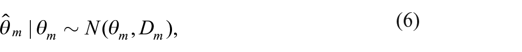
The small area models can be specified at the unit (individual or household) level; previous proposals dealing with inequality estimation are provided by Tzavidis and Marchetti (2016) and Marchetti and Tzavidis (2021) by means of robust methods. However, such models require a large amount of data as, generally, the auxiliary variables have to be known for each unit of the population and linked to survey data. This may be hard to get as administrative archives are not publicly accessible at individual level, cross-linked and associated with survey data (Harmening et al. 2023). On the other hand, small area models defined at the area level are less demanding in terms of data requirements, needing only survey (direct) estimates endowed with related measures of uncertainty and areal covariates (Rao and Molina 2015). An application of such models to inequality estimation can be found in Benedetti and Crescenzi (2023).
Area-level models in their classical specification, the Fay-Herriot model (Fay and Herriot 1979), have the strict assumption of (approximate) unbiasedness of the survey estimators given as input (Rao and Molina 2015). However, inequality estimators are biased in small samples, often underestimating inequality (Breunig and Hutchinson 2008; Deltas 2003). In this paper, we focus on such bias which may depend on the non-linear nature of inequality indicators, on the characteristic of the distribution of the variable of interest, that is, the income variable (Breunig 2001), and on the uncertainty induced by the sample selection scheme.
Unfortunately, such an issue is typically neglected when measuring inequality with area-level models, leading to model misspecification and thus to a possible misleading inference. Note that this aspect deserves attention given that estimates of inequality measures are often used for comparisons across time and locations. Neglecting it may bring out discrepancies that, rather than being true inequality gaps, may be due to disparate sample sizes or to different underlying distributions of the variable of interest (Breunig and Hutchinson 2008). In this vein, we propose a bias correction strategy for a large set of inequality measures and we adopt it in an illustrative small area estimation exercise.
Concerning the Gini index, a large body of literature faces the small sample bias issue, such as Jasso (1979), Lerman and Yitzhaki (1989), Deltas (2003), Davidson (2009), Van Ourti and Clarke (2011) in iid samples. The context of application is varied, spanning from economic inequality to crime or concentration of scholarly citations (Kim et al. 2020; Mohler et al. 2019). Fabrizi and Trivisano (2016) tackle such an issue in the complex survey case and their correction is indeed considered within a small area estimation framework. However, concerning alternative measures such as Atkinson Indexes and the Generalized Entropy (GE) measures, the literature on bias is very scarce, even in the iid case: some contributions are provided by Giles (2005), Breunig and Hutchinson (2008), Schluter and van Garderen (2009) by adopting different methodological approaches of correction.
Note that income data are collected through household surveys with complex sampling designs that adopt stratification and/or selection of sampling units in more than one stage. Thus, the sample selection process, together with ex-post treatment procedures such as calibration and imputation, invariably introduces a complex correlation structure in the data that has to be taken into account. This makes the development of a theoretically valid bias correction challenging, in contrast to classical iid settings. Furthermore, the bias issue is even exacerbated in income data applications, traditionally affected by extreme values (Van Kerm 2007), since inequality measures are known to be highly unrobust to them (Cowell and Victoria-Feser 1996). This aspect depends clearly on the type of measure we are dealing with and it becomes even more cumbersome to handle in the case of small samples.
We investigate the nature of the bias and propose a methodological framework for bias correction. Our proposal constitutes a generalization of the framework of Breunig and Hutchinson (2008), developed for iid observations, to the finite population and design-based setting. At the same time, we extend the proposal to a wider set of measures from the Gini index to two parametric families of measures: the Atkinson and the Generalized Entropy family, commonly used to measure inequality (Daly and Valletta 2006). We consider a wide variety of measures as the concurrent estimation of alternative indicators—as opposed to the more commonly used Gini Index—may bring to light a wider picture of the inequality phenomenon. This is motivated by their interesting properties such as the additive decomposability, for Generalized Entropy measures, and the explicit social welfare representation, for Atkinson measures. Moreover, all the measures considered pertain to the class of dispersion-based measures, sharing common features that enable the development of a general bias correction framework. To the best of our knowledge, this is the first proposal of bias correction for the Atkinson and Generalized Entropy indexes in the complex survey case, whereas it provides an extension for the Gini index case with respect to existing proposals as it is made clear in Section 4.
To our purpose, we take advantage of a methodology based on Taylor’s expansions, even if the same analytical results can be obtained through other types of linearization, such as the one proposed by Graf (2011). Our extension for complex designs is based on the introduction in the estimation strategy of (i) sampling weights, as to consider the unequal probabilities of selection and (ii) relevant design information, such as strata and clusters, to control for possible correlation among units. Other limitations associated with household surveys are related to non-sampling issues, such as non-response and non-representativeness, which may significantly impact the accuracy of estimates. The incorporation of sampling weights, if properly treated for non-response and calibrated to known population totals, may also protect against such issues. This is the case of the Italian EU-SILC survey data we employ in this paper (ISTAT 2021).
By considering a combination of stratified and multistage cluster sampling, the incorporation of weights is made explicit by adopting Horvitz-Thompson type estimators and the ultimate clusters technique for design variances and covariances estimation. An advantage of our proposal is that any parametric assumption on income distribution is not required, providing a very flexible framework. Our bias correction proposal is evaluated via simulations showing a noticeable bias reduction for all the measures and leading, in some cases, to approximately unbiased estimators. Results under different simulation scenarios confirm that the presence of extreme values does not seem to compromise the bias correction process. Lastly, we provide a small area estimation exercise that shows the risk of ignoring ex-ante bias correction.
The paper is organized as follows. The considered inequality measures are defined in Section 2, while the bias correction strategy is set out in Section 3 and the bias-correction estimation steps are detailed in Section 4. A design-based simulation study involving the European Statistics on Income and Living Condition (EU-SILC) income data is provided in Section 5 to evaluate the magnitude of the bias and the efficacy of our proposal. Lastly, a small area estimation exercise is carried out in Section 6, to highlight the utility of our proposal in practice. Conclusions are drawn in Section 7.
2. Inequality Measures
The most famous inequality measure is, indeed, the Gini concentration index, employed in social sciences for measuring concentration in the distribution of a positive random variable. Suppose we have a finite population U of N < ∞ elements labeled as
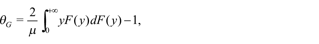
with
An explicit incorporation of social welfare in inequality measurement is given by Atkinson indexes, which provide for a complete ranking among alternative distributions at the expense of more stringent assumptions as to how to represent social welfare (Bellu and Liberati 2006). Atkinson index has support [0, 1] and is defined as
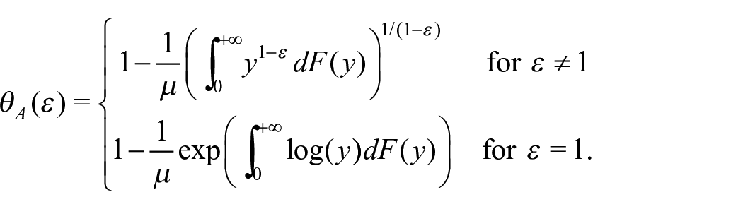
The parameter
Besides, an additive decomposable family of inequality measures is the Generalized Entropy class. As opposed to the measures seen before, this class has the advantage of being strongly transfer-sensitive, meaning that it reacts to transfers depending on donor and recipient income levels. It is based on the concept of entropy which, when applied to income distributions, has the meaning of deviation from perfect equality:
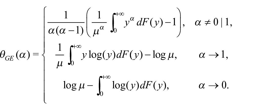
The parameter

In this paper, we consider the estimation of both classes separately, since common parameter values used in one family do not correspond deterministically to parameter values commonly used for the other family. Lastly, we consider the coefficient of variation (CV) as an inequality measure, being linked with a member of the GE family, namely
3. Bias Correction Proposal
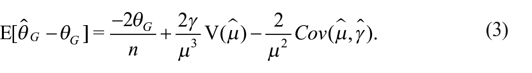
The bias of inequality estimators in small samples can be due to the structure of inequality measures as a non-linear function of estimators. The bias can be either positive or negative, depending on the characteristics of the reference variable distribution, except for the Mean Log Deviation which has a structurally negative bias as shown further on in this section. Among the measures with non-predictable bias direction, Breunig (2001) shows that the bias of CV and GE (2) is negatively related to the skewness of income distribution. This aspect could be analyzed in-depth by imposing a distributional assumption on the income variable, but this is beyond the scope of this paper. For GE and Atkinson measures, the limiting behavior of their bias is described in the following proposition.
Proposition 1. For the measures belonging to the GE and Atkinson families, the expectation of their sample estimator
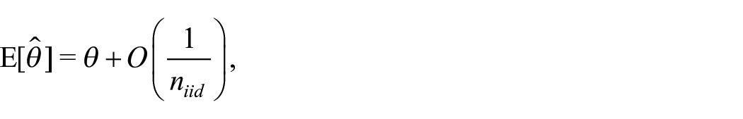
with
Proof. In appendix.
We are interested in a variety of non-linear functions of income values as inequality measures are. Let denote with
We consider the generic inequality measure written as a function of the mean m and

with
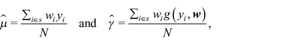
where
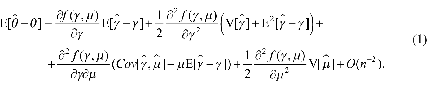
In Table 1, we detail the survey estimators for each inequality measure and their bias formulation based on Equation (1) along with all relevant quantities. The complex survey estimators of Atkinson and Generalized Entropy measures come from Biewen and Jenkins (2006), while as for the Gini index, we employ the alternative formulation defined by Sen (1997) and the complex survey estimator proposed by Langel and Tillé (2013). Let denote with
Relevant Quantities for Each Measure Including the Approximate Bias.
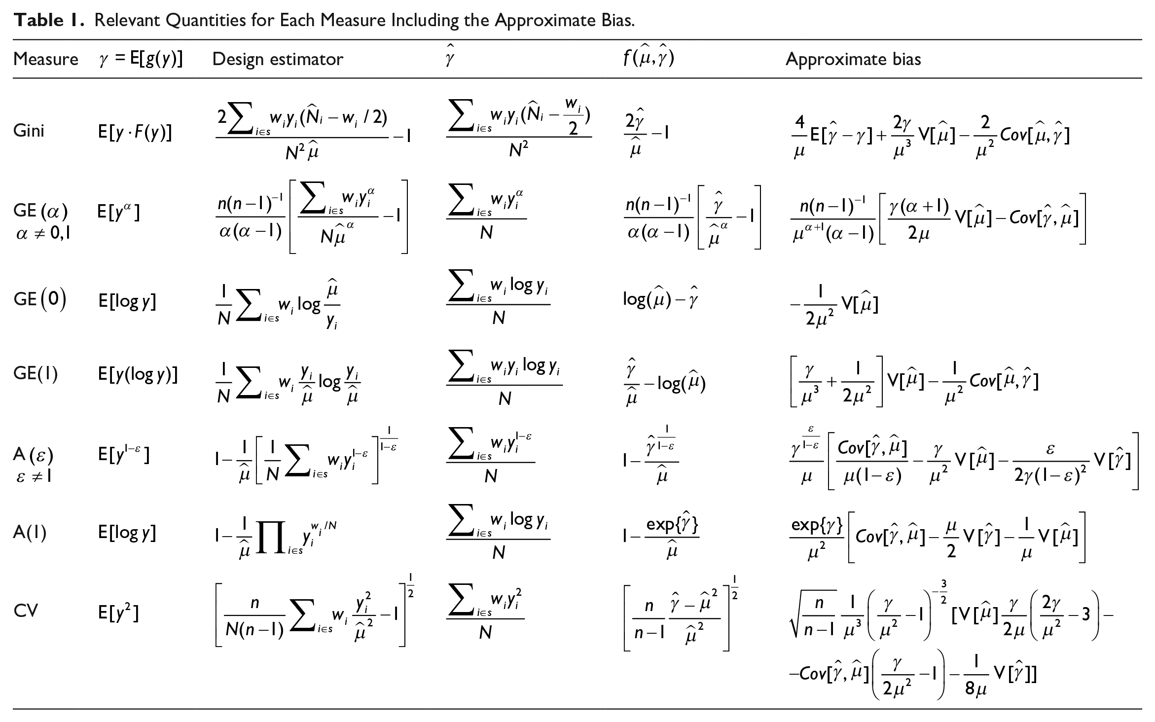
Let us denote the Gini index estimator with
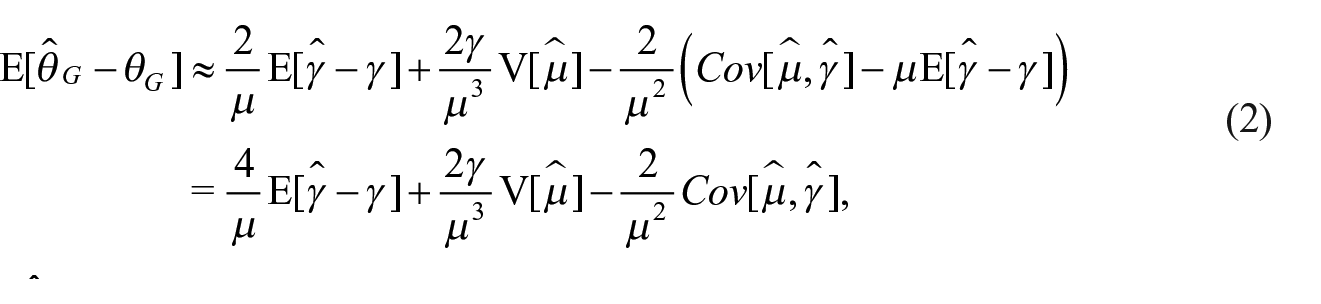
with
This correction is in line with Davidson (2009) and Fabrizi and Trivisano (2016) proposals. However these are based on a first-order Taylor’s expansions and thus limited to the first term of the right-hand side Equation (2), ours extends it to a second-order expansion. This translates into the fact that, while Jasso (1979), Deltas (2003), and Davidson (2009) proposals identify the adjusted Gini in iid context as
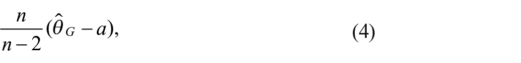
with
Note that the bias formulas of Table 1 can also be reached differently, namely by applying the linearization proposed by Graf (2011) and extended by Vallée and Tillé (2019), as made explicit in the Appendix. Graf’s methodology requires a separate derivation for each measure. In contrast, Equation (1) defines a general bias formulation of the bias that applies to the entire set of considered measures, isolating its components and easing a general interpretation. This is one of the pros of our methodology, together with the fact that it is a distribution-free procedure, not requiring any parametric assumption on income distribution. Another pro that is worth mentioning is that Taylor’s expansion in Equation (1) relies on design variance and covariances. Since uncertainty estimation of complex design estimators is of great interest, such quantities can safely be estimated in a complex survey context as several variance estimation techniques have been proposed and tested in literature. On the contrary, other methodologies, such as small-sigma or Edgeworth expansions, may require parametric assumptions on income distribution and/or the estimation of moments up to higher orders, which may be unreliable in the case of complex design data.
As is clear from Table 1, the bias correction of GE(2) does not include the coefficient of skewness of the income distribution, as shown by Breunig (2001). A reliable estimation of that quantity, while being straightforward in the iid case, appears cumbersome in the case of weighted data being defined on a discrete grid of values. This adds up to another aspect: their estimators may be particularly unstable in small samples (Joanes and Gill 1998). This leads to the non-applicability of Breunig (2001) result in our case.
4. Bias Estimation
In this section, we detail the estimation of the approximate bias defined in Table 1 for each measure. Such estimation is not trivial considering that the mentioned expressions depend on design variances and covariances
We define an unbiased estimator for the variance of Horvitz-Thompson estimators, such as m
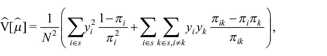
with πik,
Therefore, the variance estimator to be considered constitutes an approximation that relies on simplified assumptions. Firstly, we assume that Primary Sampling Units (PSU) are sampled with replacement, and secondly, we reduce multi-stage sampling into a single-stage process by relying on the Ultimate Clusters technique (Kalton 1979). Moreover, we take into account the hybrid nature of the probability scheme, blending a variance estimator for stratified design associated with the SR strata, including a finite population correction factor, and a typical Ultimate Cluster variance estimator for multi-stage schemes associated with the NSR strata. The latter one is widely used in official statistics, see Osier et al. (2013) for Eurostat procedures. Without loss of generality, let us consider a two-stage scheme, where
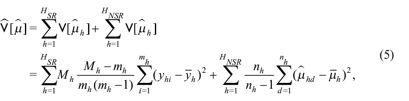
with
An estimator of
Thus, a possible estimator
The Gini index estimator differs from the other indexes since
for a generic unit
In this section, we have detailed the estimation of each quantity that contributes to the definition of the bias-corrected estimator of inequality measures. Note that the issues related to the sampling variance of bias-corrected estimators and its estimation are addressed later on in Section 6.
5. Design-Based Simulation
A design-based simulation study has been conducted to evaluate our bias correction proposal. In this simulation, the cross-section Italian EU-SILC sample (2017 wave) has been assumed as pseudo-population and the twenty-one NUTS-2 regions have been considered as target domains. The study is based on real income data, in order to check whether this specific framework works with close-to-reality data, affected by peculiar problems, for example, extreme values and skewness.
For comparison purposes, two simulation scenarios have been carried out. In the first one, the original income data are employed as pseudo-population. In the second one, an extreme values treatment is performed concerning both upper and lower tails, to circumvent non-robustness problems. The issue of robust estimation of economic indicators through an extreme values treatment in the upper tail of income distribution is well-established in the literature. See Brzezinski (2016) for a review and Alfons et al. (2013) for a suitable specification for survey data. On the contrary, the issue of treatment of extreme values in the lower tail of income distribution appears less established (Hlasny et al. 2022; Masseran et al. 2019; Van Kerm 2007).
The treatment is done at a regional level to the original EU-SILC sample and the detection of outlier is carried out by using the Generalized Boxplot procedure for skewed or heavy-tailed distributions (Bruffaerts et al. 2014). Outliers are defined as the observed values that exceed certain bounds computed by directly taking into account the skewness and tail heaviness of the distribution. Such outliers, once identified, are randomly replaced by draws from Pareto or inverse Pareto tails. On the upper tail, we operate a semi-parametric Pareto-tail modeling procedure using the Probability Integral Transform Statistic Estimator (PITSE) proposed by Finkelstein et al. (2006), which blends very good performances in small samples and fast computational implementation, as suggested by Brzezinski (2016). As regards the lower tail, we use an inverse Pareto modification of the PITSE estimator suggested by Masseran et al. (2019). The resulting dataset is specified as an alternative (hereafter, treated) pseudo-population. The number of treated observations, together with some summary statistics about survey data, can be found in the Appendix.
From both pseudo-populations, we repeatedly select 1,000 two-stage stratified samples, mimicking the sampling strategy adopted in the survey itself. In the EU-SILC survey, the first-stage is characterized by a stratified sampling of municipalities according to NUTS-2 region and population sizes. In the second-stage, households are selected within each PSU through systematic sampling. The simulation study mimics this design by approximating strata to NUTS-2 regions. We repeated the drawing for both scenarios involving different sampling rates, 1.5% and 3% respectively. Results before/after treatment are compared to isolate the effect of extreme values when evaluating bias-correction performances.
The Relative Bias (RB), Mean Square Error (MSE), its variance component percentage (%VAR) and the Root Mean Square Error (RMSE) are calculated for each region
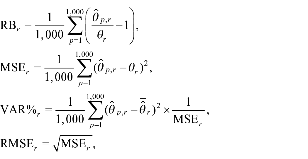
where
Concerning the treated pseudo-population scenario, Figure 1 illustrates the relative bias for each domain of non-corrected measures (gray line) and of corrected measures (blue line) in 3% samples versus the (average) sample size. The negative relation between sample size and average relative bias is clear for both the survey estimator
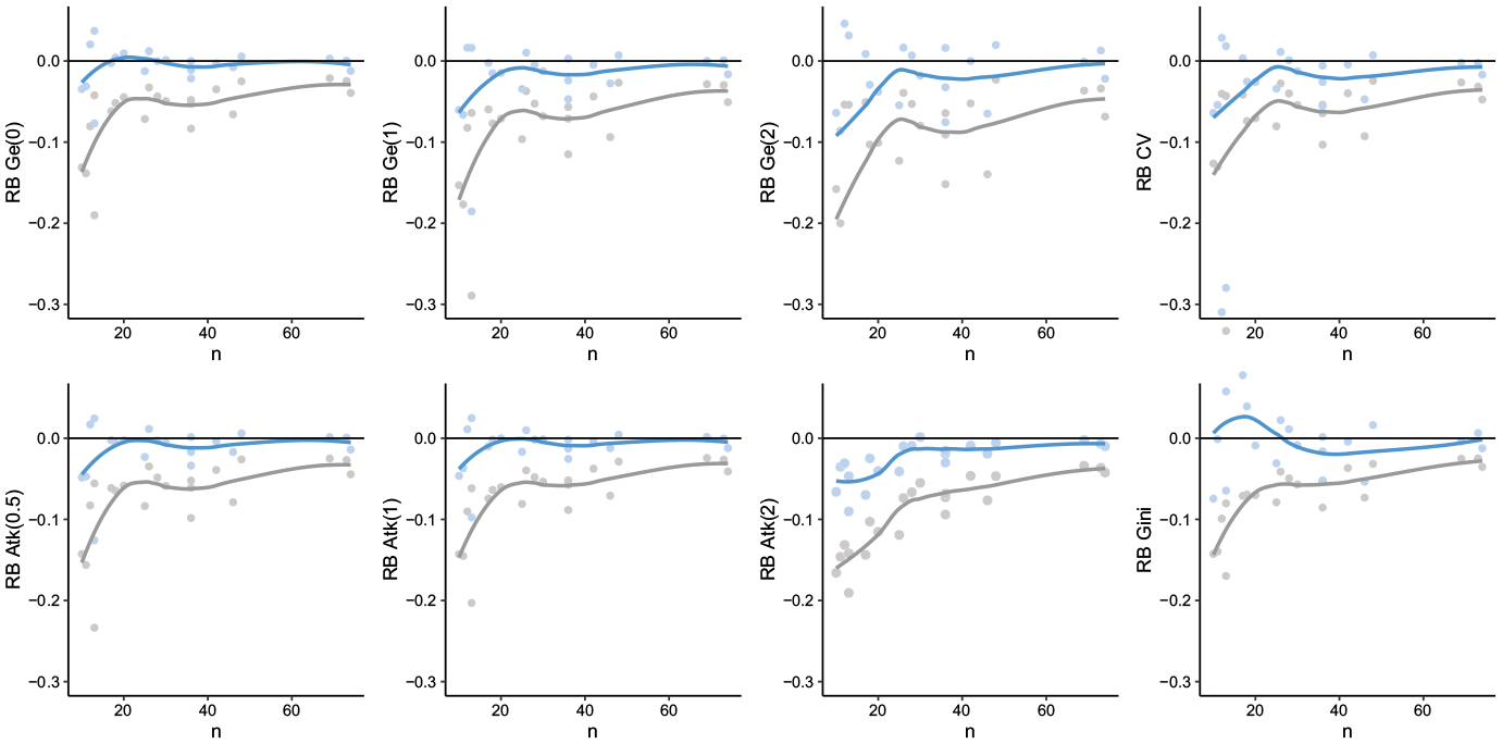
Relative Bias of non-corrected measures (gray line), and corrected measures (blue line) in 3% samples after extreme value treatment versus the (average) sample size.
Bias and error averaged across all areas for each scenario, sampling rate and estimator are shown in Table 2. By still focusing on treated population results, the correction induces a reduction of the RB spanning from 5% (CV, 3% rate) to 14% (Gini, 1.5% rate) approximately by considering both sampling rates. When the sample size is greater than 20
Percentage RB and RMSE Averaged on the Twenty-One Regions for Each Inequality Estimator and Scenario.
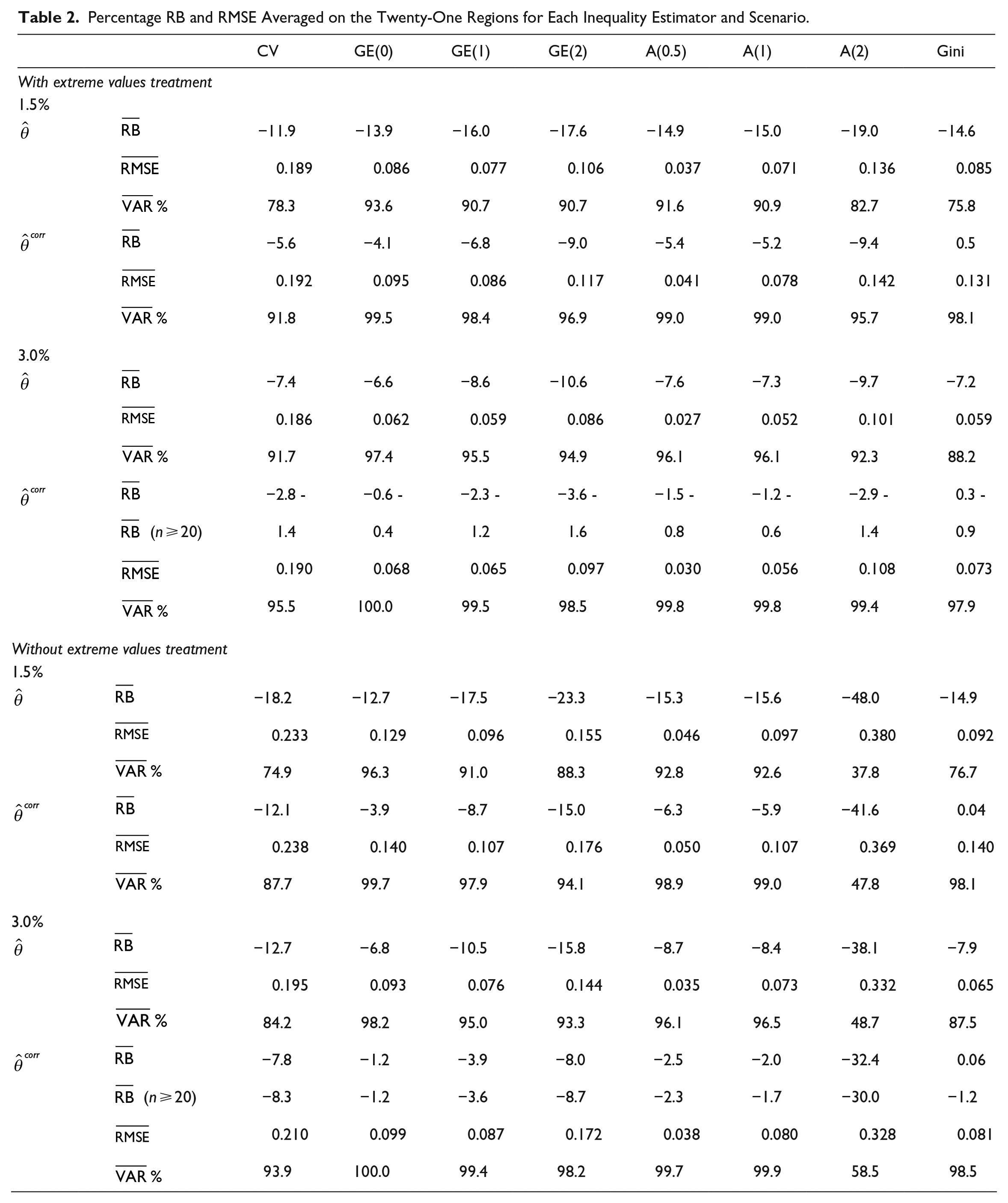
Note that the variance component percentage of MSE (%VAR) for the corrected estimators is always greater than for the non-corrected counterparts, and it reaches the 100% of MSE in some cases. This means that the error is largely due to estimators variance, while the bias has a minimal component. The price to pay for a bias correction procedure is an increase in variance; this bias-variance trade-off pushes us to a reflection. Since we are in a small sample context, both corrected and uncorrected estimators are strongly unreliable, requiring a variance reduction step. To undertake this step, the corrected estimators are preferable as their error is largely due to estimator variability
Let us focus on comparing the treated population scenario with the non-treated one. In the latter case, bias and error increase dramatically both for
To summarize, our results highlight that in the case of populations that are not affected by income extreme values, the bias correction may provide approximately unbiased estimates for a large class of measures at the expense of, in most cases, only a slight error increase. Vice versa, it might be necessary to restrict the attention to the most robust measures such as GE with
6. A Small Area Estimation Exercise
In the previous sections, we propose a method to correct the small sample bias of inequality estimators in complex surveys. Even if bias-corrected, such estimators are still unreliable due to the high variability induced by the small sample size: this means that estimates cannot be released or used for further inference. As a consequence, when measuring inequality at a fine-grained level, it becomes necessary to rely on Small Area Estimation (SAE) techniques. Such estimation techniques take advantage of available auxiliary information to produce estimates with acceptable uncertainty. More specifically, the model-based SAE techniques employ hierarchical models which can be defined both at area-level, linking area-defined survey estimates with areal covariates, or at unit (individual) level, linking individual income data with individual covariates. See Tzavidis et al. (2018) for an up-to-date review.
In this context, area-level models appear to be less demanding in terms of data requirements and enable the incorporation of design-based properties. Such models constitute a typical framework for the application of our bias-correction proposal, as they assume the unbiasedness of survey estimators used as input. As a consequence, their applicability to the estimation of inequality measures is inevitably tied to a preliminary bias correction, in contrast with unit-level models that do not involve survey estimators.
In this section, we perform an SAE exercise by measuring inequality in specific small domains through the 2017 Italian EU-SILC data, already employed in Section 5. The domains considered are the interaction between five NUTS-1 regions (North-East, North-West, Center, South, Insular), three DEGURBA classification types (Urban, Peri-urban, and Rural), and six household types (one-member households, lone parents with one or two dependent children, lone parents with three or more dependent children, couples with one or two dependent children, couples with three or more dependent children, households without dependent children). As dependent children, we mean sons/daughters aged less than twenty-five. This allows the estimation of inequality for geographics domains and specific sub-population of interest such as household types.
The purpose is not to propose a small area estimation strategy but rather to illustrate the framework of application of our bias-correction proposal and, especially, to underline the risk of avoiding bias-correction when estimating inequality in small domains. Such exercise is carried out by applying the Fay-Herriot model (Fay and Herriot 1979), a landmark model in the small area literature, implemented through the package sae (Molina and Marhuenda 2015) to both uncorrected and corrected survey estimators. The objective is to check whether the inclusion of biased or bias-corrected survey estimates in the model may lead to different results. We perform the exercise on the most popular estimators among the ones previously considered: the Theil index (Generalized Entropy with
Specifically, let us consider
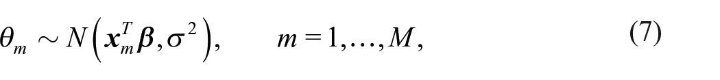
where
As mentioned above, the design variance is separately estimated from the data and given as input to the small area model: its estimation in real application is the crux of an SAE procedure. In the case of uncorrected inequality estimators, it may be easily carried out via linearization. Linearized variables for each measure could be derived consistently with Langel and Tillé (2013) for the Gini index and Biewen and Jenkins (2006) for the Generalized Entropy and the Atkinson indexes. On the other hand, the variance of bias-corrected estimators adds a new level of complexity since the estimator formula is no longer the classical one. Indeed, it comprises a bias correction component that appears cumbersome to estimate via linearization since it is inherently a result of several linearizations. Therefore, we recommend relying on resampling methods; a comprehensive review of the use of bootstrap methods for survey data can be found in Lahiri (2003). In this case, we employed the design-aware bootstrap procedure as presented by Fabrizi et al. (2011, 2020). The algorithm involves both a drawing procedure that considers the multi-stage selection process and a calibration procedure, applied to each bootstrap sample, that adjusts weights with respect to known totals. A similar process is performed to the original EU-SILC sample by national statistical offices.
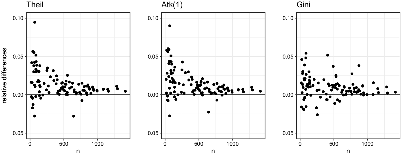
The comparison between uncorrected and corrected survey estimates for all three measures is displayed in relative differences, that is,
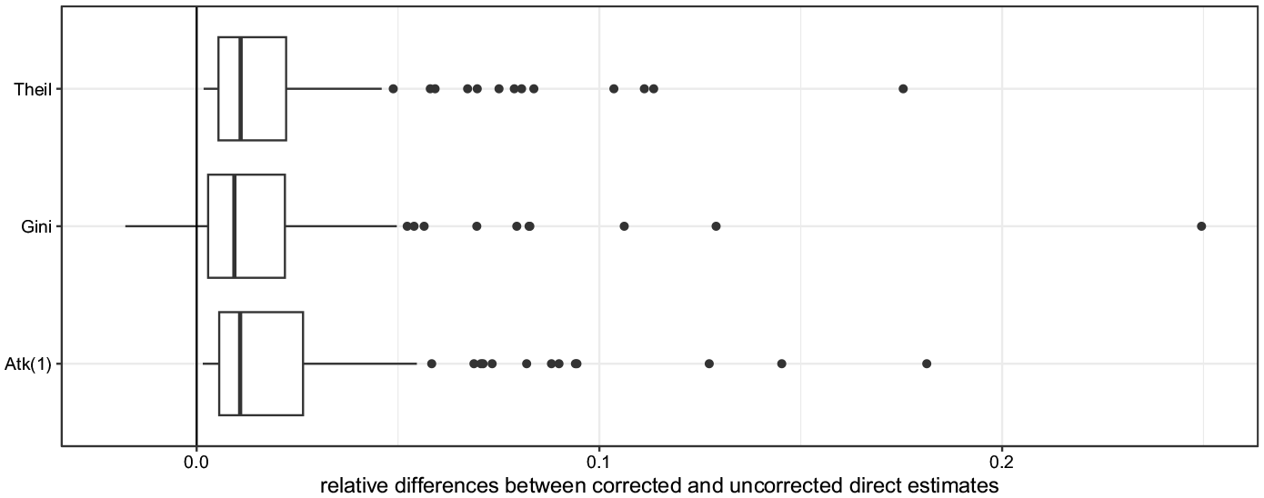
Relative differences between corrected and uncorrected direct estimates for each measure.
We separately fit the Fay-Herriot model for both corrected and uncorrected estimators by using the same set of covariates. We consider only covariates defined for the geographical area of interest of the domains: the aged dependency ratios from census data and the average values and incidence by income source from tax forms data. Indeed, due to data disclosure issues, it is not possible to retrieve the disaggregated information by household type. Such covariates are subjected to variable selection to avoid multicollinearity and to neglect irrelevant regressors. The final set includes (i) the age dependency ratio, measuring the population aged between zero and fourteen over the total population, being positively related to inequality, (ii) the average income declared by entrepreneurs, and (iii) the employee income incidence, both negatively related to inequality. The model-based (or EBLUP, Empirical Best Linear Unbiased Predictor) estimates in both cases are compared in terms of relative differences in Figure 3. The inequality levels estimated by the misspecified model are lower in most of the cases, resulting in a misleading inference. The greatest divergences show that the model-based estimate resulting from an ex-ante bias correction is 11.4% higher than the one without correction. This confirms the risk of underestimation of inequality when neglecting such an issue. As expected, the divergences between model-based estimates in both cases decrease to zero at increasing sample sizes.
Sample sizes versus relative differences between model-based estimates based on corrected survey estimates and model-based estimates based on uncorrected ones.
By focusing only on EBLUP results based on corrected estimates, the decrease in terms of error induced by the model is depicted in Figure 4. The reduction is relevant and testifies that the variance reduction procedure, put in place by the SAE model, is effective. As a consequence, such model-based estimates result to be reliable and ready to be used for further analysis or mapping.
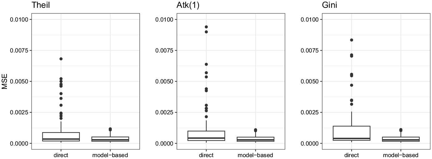
MSE of inequality estimators. Bias-corrected direct estimators versus model-based estimators.
7. Conclusions
A strategy based on Taylor’s expansion has been proposed to correct the small sample bias of inequality estimators. The inequality measures considered are several, as the comparison of diverse measures may enable us to enlighten the specific point of view that each measure provides, like single tiles in a mosaic. Indeed, the well-known Gini and Theil indexes are widely applied in several fields for inequality and concentration estimation.
A sensitivity analysis with respect to outliers and a simulation study have been conducted to study the estimator behavior to extreme values and the performance of the proposed correction. Results show that survey-based estimators may be biased in small samples, inducing an underestimation that is even greater in the case of populations affected by extreme values. Moreover, simulation results validate the correction proposal as effective, consistently reducing the bias and leading in some cases to approximately unbiased estimators.
An underlined heterogeneity of sensitivities and bias is recorded across measures. As a consequence, our results may help in choosing the most suitable inequality measure depending on the context. The measures that are structurally more sensitive to extreme values appear to be more biased, in particular, GE with
An illustrative small-area application has been carried out to evaluate the effect of disregarding bias in a typical small-sized sample context. The results obtained show that neglecting it translates into a misleading inference and inequality underestimation. In such an application, we use a basic area-level model, the Gaussian one. Indeed, the possibly not-Gaussian sampling distributions of inequality estimators and the unit-interval support of Gini and Atkinson estimators might urge a more refined model, which may lead to model-based estimators with increased performances: this suggests an interesting direction for future research. Further directions also include the extension of this framework to other widely used inequality measures, such as those based on quintiles and the development of a multivariate SAE framework.
Footnotes
Appendix
Funding
The author(s) disclosed receipt of the following financial support for the research, authorship, and/or publication of this article: The work of Silvia De Nicolò was partially funded by the ALMA IDEA 2022 grant (title: “Social exclusion and territorial disparities: poverty and inequality mapping through advanced methods of small area estimation,” project J45F21002000001) and by the PNRR PE10 ONFOOD project (title: “Research and innovation network on food and nutrition Sustainability, Safety and Security – Working ON Foods,” project J33C22002860001). Part of the European Union—NextGenerationEU funding. The work of Maria Rosaria Ferrante was funded by the European Union - NextGenerationEU, in the framework of the “GRINS -Growing Resilient, INclusive and Sustainable project” (PNRR - M4C2 - I1.3 - PE00000018 – CUP J33C22002910001). The views and opinions expressed are solely those of the authors and do not necessarily reflect those of the European Union, nor can the European Union be held responsible for them.
Received: March 2023
Accepted: December 2023