Defining Ad-Hoc Sampling Designs for Small Area Estimation

Abstract

The paper sketches a proper statistical setting necessary to define the sampling design for Small Area Estimation (SAE). Since SAE techniques are commonly used in official statistics, relying on appropriate sampling designs to improve the quality of estimates becomes crucial. The sampling design is based on both allocation and sampling selection. The allocation step solves a non-standard problem necessary for finding the minimum-cost solution that controls the accuracy of the model-based small area estimator. The sampling selection ensures the planned sample sizes for each level of random effects affecting the variables of interest.

1. Introduction

The paper outlines a proper statistical setting necessary to define the sampling design for Small Area Estimation (SAE). An area (or domain) is considered small if a direct estimator based on the sampling design, for example, the Horvitz-Thompson estimator (Särndal et al. 1992), produces unreliable estimates. Let us imagine that we do not observe a domain in the sample. In this case, we cannot compute the direct estimate since the applicability of the estimator depends on the presence of sampling units in the domain of interest (Lehtonen et al. 2003; Lehtonen and Veijanen 2009; Rao and Molina 2015). According to a model-based approach, we usually treat the SAE problem via indirect estimation exploiting the values of the variable of interest $y$ also from different areas or the same area but using data from previous survey occasions (Rao and Molina 2015). This approach does not consider sampling design issues.

In this paper, we use another approach and investigate the issues of how to define a random sampling design and selecting the sample units in the case where we estimate the characteristics of interest at the domain level with SAE techniques developed under a model-based approach to inference (Chambers and Clark 2012). We try to define a random sampling strategy consistent with the adopted estimation method. In essence, the strategy we propose seeks to plan and select the sample in the best possible way to guarantee, within the available budget, predefined levels of accuracy for model-based estimates by domain. In our approach, we propose controlling the sample size at each level of the random effects considered in the SAE model used for estimation. For instance, if the SAE model includes a random effect for each small area of interest, the sampling design could specify a targeted sample size for each small area. Conversely, if the model assumes random effects only at the level of broader macro-areas, the sampling design should be adjusted to allocate sample sizes appropriately for those macro-areas. This approach ensures more accurate model-based estimates compared to scenarios where some levels are not observed in the sample. This condition provides more accurate model-based estimates than the situation where we do not observe some levels in the sample. A significant result we provide is the definition and the algorithmic solutions to the non-standard problem for identifying the inclusion probabilities as the result of a minimum cost problem, ensuring predefined thresholds for the accuracy of small area estimates.

Dealing with the problem of defining the sampling design when using the SAE techniques may sound strange, given that these techniques were created to overcome the insufficient sample sizes of the domains that were not planned at the moment of the survey design. However, in the last few decades, a growing number of national statistical institutes and other statistical organizations worldwide have recognized the value of regularly producing small-area statistics and using them to provide information for policy-making decisions (Kordos 2014). Some small-area estimates have been recognized as official national statistics. Two examples refer to the United Kingdom (Tzavidis et al. 2018) include the annual set of unemployment estimates for unitary authorities and local authority districts, broken down by gender and age group, and the average income estimates for electoral wards. In more than 20 developing countries, the World Bank has used SAE techniques to create poverty maps (Bedi et al. 2007). Another relevant example is the yearly dissemination of employment and unemployment statistics at a municipality level for the Italian Permanent Population Census (UNECE 2018). Furthermore, Article 9 of “Regulation (EU) 2019/1700 of the European Parliament and of the Council of 10 October 2019” includes SAE methods, intended to cover the territorial diversity, provided that they fulfill the prefixed precision requirements. In synthesis, official statistics organizations regularly disseminate estimates for small areas using SAE techniques. Therefore, it becomes relevant to develop the suggestion by Singh et al. (1994), as they noted a need to create an overall strategy that deals with the SAE problem, involving planning sample design and estimation aspects.

A consolidated approach (see Chambers and Clark 2012; Dorfman and Valliant 2005; Valliant et al. 2000) to construct the overall strategy recommends selecting a random sample and using the models to predict values for the non-sampled units of the population. Indeed, in such model-based inference, it is crucial to guard against problems arising from model failure.

Marker (2001) first contributed to defining a sampling design as it urged spreading the sample design across potential small areas to improve their estimation. It also provided examples of requiring the sample to be selected from each small area known in advance. An easily practicable way to control the sample at the level of the small areas known in advance is to adopt stratified designs where the intersection of the small areas and other design variables defines the layers. We call these cross-stratified designs. However, in many practical situations, this design is unsuitable since it requires selecting a huge number of sampling units as large as the product of the number of categories of the stratification variables (Cochran 1977, 124). Falorsi and Righi (2008) and Falorsi and Righi (2015) overcame the weakness of the cross-classified stratified design, introducing the use of the incomplete stratified design. This approach controls the sample sizes for the marginal strata, corresponding to the domain partitions, while the sample size in the cross-classified strata is a random variable. The proposed strategy uses a balanced selection technique (Deville and Tillé 2004). The sample allocation specifies the sample sizes in the marginal strata to ensure that the sampling errors of the domain estimators are lower than pre-specified thresholds. Moreover, in Falorsi and Righi (2015), a GREG-type estimator is adopted (Lehtonen et al. 2003; Lehtonen and Veijanen 2009). Furthermore, Falorsi and Righi (2008) extended this strategy to synthetic estimators and, more generally, to model-based estimation. Burgard et al. (2014) and Friedrich et al. (2018) focused on a topic related to optimal SAE sampling. In both papers, the authors highlight the need to provide samples at the domain levels and a variety of subclasses. The use of cross-classified stratified design leads to a too-detailed stratification of the population. Optimizing the accuracy of design-based estimator for stratified random samples requires incorporating many strata at various levels of aggregation. Considering several variables of interest for the optimization yields a multivariate optimal sampling allocation. In particular, Burgard et al. (2014) studied the effect of some SAE sampling designs for business data and suggest considering the box-constraint optimal allocation proposed by Gabler et al. (2012). Rao and Molina (2015, Section 2.6) advocate for effective sampling designs to improve small area estimation. Their key proposals include minimizing clustering to enhance effective sample size, using stratification to create smaller strata for better data quality, and implementing compromise sample allocations for reliability across small and large areas. They also suggest employing dual-frame surveys and harmonizing questions across surveys to increase effective sample sizes. Keto et al. (2018) recommended a sampling allocation based on multi-objective optimization using a small-area model and estimation method introduced by Falorsi and Righi (2008). Breidt and Chauvet (2012) review balanced sampling and the cube algorithm, proposing an implementation that allows the selection of penalized balanced samples. Such samples can lessen or even remove the need for linear mixed model weight adjustments and yield highly efficient Horvitz–Thompson estimators when responses are well captured by a linear mixed model with auxiliary information. Finally, at the end of this short bibliographic review, the work of Pfeffermann and Ben-Hur (2019) is worth mentioning as well. They contributed to the topic of joint use of random sampling and model-based inference by proposing a hybrid inferential approach to estimating the design-based mean squared error of model-dependent small area predictors. Having adequate and general measures of the mean squared errors in this context is important in order to be able to produce accurate measures of the quality level of the estimates produced.

Our proposed solution addresses the SAE problem through three key steps: (1) defining a budget-aligned SAE working model that balances complexity and feasibility, (2) optimizing inclusion probabilities for cost-effective allocation while maintaining model-based accuracy, and (3) employing balanced sample selection techniques to account for random effects and auxiliary variables. This comprehensive strategy enhances SAE estimate accuracy through an improved sampling design. Additionally, we introduce an algorithm to solve the optimization problem and demonstrate its practical implementation with a case study based on real data and a simulated dataset.

The article is organized as follows. Section 2 formalizes the statistical and mathematical aspects of the problem at hand. Section 3 shows traditional small area estimation models that could be implemented in line with our proposal. Section 4 proposes a formulation for the sampling optimization problem. Section 5 presents empirical evidence based on a simulated and real datasets. Finally, Section 6 offers some concluding remarks.

2. Statistical Setting

2.1. Parameters of Interest

Let $U$ be a population of size $N$ , and let $U_d(d=1,\dots ,D)$ be a particular sub-population of $U$ of size $N_d$ . The target parameters are the domain-level means of one or more variables of interest

$${\overline{Y}}_{\mathrm{vd}}=\frac{1}{N_d}\sum _{i\in U}{y}_{\mathrm{vi}}{\lambda }_{\mathrm{di}}=\frac{1}{N_d}\sum _{i\in U_d}{y}_{\mathrm{vi}}$$

(2.1)

where $y_{\mathrm{vi}}$ $(v=1,\dots ,V;i=1,\dots ,N)$ indicates the value of the variable of interest ${\mathcal{y}}_v(v=1,\dots ,V)$ in the $i$ -th $(i=1,\dots ,N)$ unit of the population $U$ and ${\lambda }_{\mathrm{di}}(d=1,\dots ,D;i=1,\dots ,N)$ is the domain membership variable, where ${\lambda }_{\mathrm{di}}=1$ if $i\in U_d$ , and ${\lambda }_{\mathrm{di}}=0$ otherwise. Equation (2.1) identifies a multivariate-multi-domain schema. Indeed, there are $V$ (variables $)\times D$ (domains) target means. Finally, let ${\mathit{x}}_i={(x_{1i},\dots ,x_{\mathrm{Pi}})}^{\prime }$ be a vector of $P$ auxiliary variables known for all population units.

2.2. Sampling

We assume for now that the domain membership variables are available in the sampling frame and observable without measurement error. We observe the variables of interest ${\mathcal{y}}_v(v=1,\dots ,V)$ on a random sample $S$ of fixed size $n$ selected from the population $U$ with the vector $\mathit{\pi }={({\pi }_1,\dots ,{\pi }_i,\dots ,{\pi }_N)}^{\prime }$ of inclusion probabilities. Let $S_d\equiv \cap S{U}_d$ be the subset of sample units belonging to the population $U_d$ . $n_d$ is the number of units in $S_d$ .

We select the sample $S$ with the Cube algorithm (Deville and Tillé 2004), respecting, at least approximately, the following balancing equations:

$$\sum _{i\in S}\frac{{\mathit{b}}_i}{{\pi }_i}\cong \sum _{i\in U}{\mathit{b}}_i$$

(2.2)

where ${\mathit{b}}_i$ is a vector of auxiliary variables for the unit $i$ . We define the variables ${\mathit{b}}_i$ such that precisely $n_d$ units are selected in each sample selection, where $n_d$ is an integer.

Let ${\mathbf{\lambda }}_i={({\lambda }_{1i},\dots ,{\lambda }_{\mathrm{di}},\dots ,{\lambda }_{\mathrm{Di}})}^{\prime }$ be a known column vector of $D$ entries. Deville and Tillé (2004, 895 and 905) demonstrate that if $\mathit{n}=\sum _{i\in U}{\pi }_i{\mathbf{\lambda }}_i$ , is a vector if $D$ integers, and we define the balancing variables in Equation (2.2) as

$${\mathit{b}}_i={\pi }_i{\mathbf{\lambda }}_i,$$

(2.3)

then Equation (2.2) is fully satisfied and the sampling selection ensures the planned sample sizes, $n_d(d=1,\dots ,D)$ for each domain. A rounding problem must be solved to ensure that the vector $\mathit{n}=\sum _{i\in U}{\pi }_i{\mathbf{\lambda }}_i$ is a vector of integers. Deville and Tillé (2005, 577) and Tillé and Favre (2005, 168) have shown that several customary sampling designs may be considered as special cases of balanced sampling, by properly defining the vectors $\mathit{\pi }$ and ${\mathbf{\lambda }}_i$ .

Let ${\overline{\mathit{X}}}_{\mathrm{ds}}=n_d^{-1}\sum _{i\in S}{\mathit{x}}_i{\lambda }_{\mathrm{di}}$ , and ${\overline{\mathit{X}}}_d=N_d^{-1}\sum _{i\in U}{\mathit{x}}_i{\lambda }_{\mathrm{di}}$ be the domain means of auxiliary variables respectively for the sample and the whole population. Consider the case where the values of the inclusion probabilities for the units of domain $U_d$ are sufficiently homogeneous among each other and approximately equal to $n_d/N_d$ . In that case, if the balancing variables in Equation (2.2) are defined as

$${\mathit{b}}_i={\pi }_i{({\mathbf{\lambda }}_i^{\prime },{\mathit{x}}_i^{\prime })}^{\prime },$$

(2.4)

then the selected sample respects the planned sample sizes $\mathit{n}$ , and, at least approximately, the conditions ${\overline{\mathit{X}}}_{\mathrm{ds}}\cong {\overline{\mathit{X}}}_d$ . Indeed, we have

$$\sum _{i\in S}\frac{{\pi }_i{\mathit{x}}_i{\lambda }_{\mathrm{di}}}{{\pi }_i}=\sum _{i\in S}{\mathit{x}}_i{\lambda }_{\mathrm{di}}={\overline{\mathit{X}}}_{\mathrm{ds}}{n}_d\mathrm{and}\sum _{i\in U}{\pi }_i{\mathit{x}}_i{\lambda }_{\mathrm{di}}\cong \sum _{i\in U}{\mathit{x}}_i{\lambda }_{\mathrm{di}}\frac{n_d}{N_d}={\overline{\mathit{X}}}_d{n}_d.$$

Finally, we note that the Local Cube method (Grafström and Lundström 2013; Grafström et al. 2012) is a helpful enhancement to the Cube algorithm in our setting since it enables the selection of samples that are balanced on several auxiliary variables and, at the same time, is well-spread for some variables, which can be geographical coordinates.

The proposed design employs unequal inclusion probabilities but is noninformative for the model based on the selected sample. According to Särndal et al. (1992, Section 2.4.4), Chambers and Clark (2012, Section 1.4), and Rao and Molina (2015, Section 7.6.3) this means that once we condition on the sample $S$ , the same superpopulation model that applies to the entire population is also valid for the sample units. More formally, the joint conditional distribution of the sample ${\mathcal{y}}_v$ values, given the population values of ${\mathit{x}}_i$ , is equivalent to the population distribution of ${\mathcal{y}}_v$ given the population values of ${\mathit{x}}_i$ . This equivalence holds because the ${\mathit{b}}_i$ design values—which consist of the domain membership variables and possibly the ${\mathit{x}}_i$ values—are the same basis upon which model inference is established.

2.3. Estimation

The estimation of ${\overline{Y}}_{\mathrm{vd}}$ is based on the super-population small-area model that connects the sampled values $y_{\mathrm{vi}}$ to the available covariate vectors ${\mathit{x}}_i$ . The basic unit-level model (Rao 2003, Section 7.2.1) is the simplest model we are considering in this case:

$$y_{\mathrm{vi}}={\mathit{x}}_i^{\prime }{\mathit{\beta }}_v+u_{\mathrm{vd}}+e_{\mathrm{vi}},\mathrm{for}i\in U_d$$

(2.5)

where ${\mathit{\beta }}_v$ is the regression coefficient vector, $u_{\mathrm{vd}}$ indicates a random domain effect, and $e_{\mathrm{vi}}$ is a random noise. The random domain effects $u_{\mathrm{vd}}$ are independently and identically distributed with model-expectation and variance given by $E_M\left(u_{\mathrm{vd}}\right)=0$ and $V_M\left(u_{\mathrm{vd}}\right)={\sigma }_{\mathrm{vu}}^2$ . The random individual effects $e_{\mathrm{vi}}$ are also independently and identically distributed with $E_M\left(e_{\mathrm{vi}}\right)=0$ , and $V_M\left(e_{\mathrm{vi}}\right)=$ ${\sigma }_{\mathrm{ve}}^2$ . Under the model in Equation (2.5), it is assumed that domain random effects and individual random effects are mutually independent. With negligible $n_d/N_d$ , and assuming that the variance components ${\sigma }_{\mathrm{vu}}^2$ and ${\sigma }_{\mathrm{ve}}^2$ , are known, the Best Linear Unbiased Predictor (BLUP) of ${\overline{Y}}_{\mathrm{vd}}$ is given by:

$${\tilde{\overline{Y}}}_{\mathrm{vd}}={\overline{\mathit{X}}}_d^{\prime }{\tilde{\mathit{\beta }}}_v+{\tilde{u}}_{\mathrm{vd}}$$

(2.6)

where ${\tilde{\mathit{\beta }}}_v$ is the Best Linear Unbiased Estimate (BLUE) of ${\mathit{\beta }}_v$ , ${\tilde{u}}_{\mathrm{vd}}$ is the BLUP of $u_{\mathrm{vd}}$ (Rao and Molina 2015). The model mean-squared error of ${\tilde{\overline{Y}}}_{\mathrm{vd}}$ is

$$\mathrm{MSE}\left({\tilde{\overline{Y}}}_{\mathrm{vd}}\right)=E_M{({\tilde{\overline{Y}}}_{\mathrm{vd}}-{\overline{Y}}_{\mathrm{vd}})}^2=g{1}_{\mathrm{vd}}+g{2}_{\mathrm{vd}},$$

(2.7)

where

$$g{1}_{\mathrm{vd}}=\frac{{\sigma }_{\mathrm{vu}}^2{\sigma }_{\mathrm{ve}}^2}{n_d{\sigma }_{\mathrm{vu}}^2+{\sigma }_{\mathrm{ve}}^2}=\frac{{\sigma }_{\mathrm{ve}}^2}{n_d}{\gamma }_{\mathrm{vd}},$$

(2.8)

$$g{2}_{\mathrm{vd}}={({\overline{\mathit{X}}}_d-{\gamma }_{\mathrm{vd}}{\overline{\mathit{X}}}_{\mathrm{ds}})}^{\prime }{\sigma }_{\mathrm{ve}}^2{\mathit{A}}_v^{-1}({\overline{\mathit{X}}}_d-{\gamma }_{\mathrm{vd}}{\overline{\mathit{X}}}_{\mathrm{ds}}),$$

(2.9)

where

$${\gamma }_{\mathrm{vd}}=\frac{{\sigma }_{\mathrm{vu}}^2}{({\sigma }_{\mathrm{ve}}^2/n_d)+{\sigma }_{\mathrm{vu}}^2},$$

(2.10)

$$\mathrm{being}{\mathit{A}}_v\sum _{i\in \cap S{U}_k}{\mathit{x}}_i{\mathit{x}}_i^{\prime }-n_k{\gamma }_{\mathrm{vk}}{\overline{\mathit{X}}}_{\mathrm{ks}}\overline{\mathit{X}}{\prime }_{\mathrm{ks}}),$$

where the index $k$ in the previous equation represents the generic domain, which ranges from 1 to $D$ .

The $g{1}_{\mathrm{vd}}$ component in the MSE decomposition refers to the model-based variance of the predictor ${\tilde{\overline{Y}}}_{\mathrm{vd}}$ , assuming that all model parameters (like ${\mathit{\beta }}_v$ , ${\sigma }_{\mathrm{vu}}^2$ , and ${\sigma }_{\mathrm{ve}}^2$ ) are known. Specifically, $g{1}_{\mathrm{vd}}$ reflects the uncertainty that arises within the structure of the model itself, due to both the area-specific random effects and the individual-level errors. It corresponds to the variance of the BLUP and does not account for additional variability introduced by estimating the model parameters. In this sense, $g{1}_{\mathrm{vd}}$ represents the ideal or baseline MSE of the predictor, capturing the prediction error that would remain even under perfect knowledge of the model’s parameters.

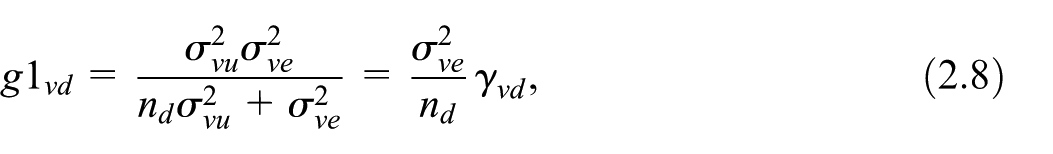
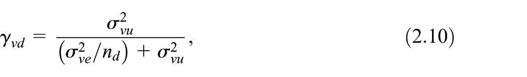
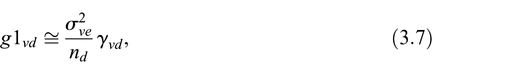
$g{1}_{\mathrm{vd}}$ is the dominant component of $\mathrm{MSE}({\tilde{\overline{Y}}}_{\mathrm{vd}})$ (Chambers and Clark 2012, 171). It is of order $n_d^{-1}(N_d-n_d{)}^2$ . In contrast, $g{2}_{\mathrm{vd}}$ is of order $n^{-1}(N-n{)}^2$ . Under specification Equation (2.3) of the balancing equations, we have $\sum _{i\in U}{\pi }_i{\lambda }_{\mathrm{di}}=\sum _{i\in S}{\lambda }_{\mathrm{di}}=n_d$ . Upon substituting $\sum _{i\in U}{\pi }_i{\lambda }_{\mathrm{di}}$ for $n_d$ in Equations (2.8) and (2.10), we observe that $g{1}_{\mathrm{vd}}$ is a function of the probability of inclusion ${\pi }_i$ . The term $g{2}_{\mathrm{vd}}$ depends on both the inclusion probabilities and the values of auxiliary $\mathit{x}$ variables for the $d-\mathrm{th}$ domain in the population and the selected sample. After data collection, we can estimate the components ${\sigma }_{\mathrm{ve}}^2$ and ${\sigma }_{\mathrm{vu}}^2$ based on sampling data. We can therefore obtain the EBLUP estimator of ${\overline{Y}}_{\mathrm{vd}}$ , where the estimates of variance components ${\hat{\sigma }}_{\mathrm{ve}}^2$ and ${\hat{\sigma }}_{\mathrm{vu}}^2$ substitute the unknown values ${\sigma }_{\mathrm{ve}}^2$ and ${\sigma }_{\mathrm{vu}}^2$ . The MSE of the EBLUP estimator, ${\hat{\overline{Y}}}_{\mathrm{vd}}$ , in this case, is equal to Equation (2.7) with the addition of the term $g{3}_{\mathrm{vd}}$ . This latter incremental variability term arises from the need to estimate the variance components ${\sigma }_{\mathrm{ve}}^2$ and ${\sigma }_{\mathrm{vu}}^2$ (see Rao 2003, 104). Then, we have $\mathrm{MSE}\left({\hat{\overline{Y}}}_{\mathrm{vd}}\right)+g{3}_{\mathrm{vd}}$ , where the term $g{3}_{\mathrm{vd}}$ , like $g{2}_{\mathrm{vd}}$ , is of a lower order than the dominant term $g{1}_{\mathrm{vd}}$ .

At the end of this Subsection, we note that the selection of auxiliary variables impacts the estimation of residual variance components ( ${\sigma }_{\mathrm{ve}}^2\mathrm{and}{\sigma }_{\mathrm{vu}}^2$ ). The allocation algorithm, which will be introduced later, will automatically account for the variance components resulting from the selected variables.

2.4. Remark 2.1. Domain Membership Variables

In some cases, domain membership variables are available in the sampling frame, particularly for business statistics where extensive data is available. This hypothesis may also apply to household surveys in European countries where population registries have demographic data attached to each person. However, in Subsections 3.2.4 and 4.2.4, we will remove this assumption to consider a more general setting. This setting is applicable to many household surveys where uncertainty exists regarding the domain membership of the population units.

2.5. Better Specification of the Objectives of the Paper

The primary objective of this article is to determine the optimal value of the inclusion probabilities vector $\mathit{\pi }$ , which guarantees a minimum-cost solution while ensuring that the values of $g{1}_{\mathrm{vd}}$ remain below the predefined error thresholds. By doing so, we aim to control the dominant part of the MSE. The optimality characteristics of the sampling design are driven by the employed model-based estimator. The statistical framework we propose in the following sections guarantees the consistency of the estimation phase with the planned sampling design. In our developments, we will consider the ${\sigma }_{\mathrm{ve}}^2$ and ${\sigma }_{\mathrm{vu}}^2$ variance components as known. As in the case of Neyman’s optimal allocation, this approach is typically adopted when defining the sample optimality in the sampling design phase. Cochran (1977, Ch. 5) observes, in the case of stratified sampling, that the optimal solution is scarcely influenced by minor deviations of the starting variances. This case also occurs in the simulation developed in Section 5, in which the MSE of the EBLUP calculated in the estimation phase is slightly higher than the MSE defined in the planning phase of the sampling design. In actual survey situations, the ${\sigma }_{\mathrm{ve}}^2$ and ${\sigma }_{\mathrm{vu}}^2$ variances can be estimated either from previous surveys or pilot surveys.

3. Super-Population Models

Following the framework proposed by Tzavidis et al. (2018, 928), the model choice should be guided by the principle of parsimony: “one should be looking to use the simplest possible method that achieves acceptable precision. Parsimony may be defined in terms of a hierarchy of estimation methods in increasing order of complexity.” The principle of parsimony suggests that during the sampling design stage, it is difficult to define complex models without actually observing the selected sample. Hence, it is best to aim for an efficient sampling design based on elementary models. Advanced models can be specified after data collection, which will help increase the efficiency defined during the sampling design stage.

In Section 3.1, we follow the principle of parsimony and discuss the basic unit-level model Equation (2.5). This model provides a reasonable basis for defining the essential aspects of the sampling design. Equation (2.5) is applicable in situations where the areas are small geographic areas. In such cases, the model allows for units in the same geographic location to be correlated through the random effect $u_{\mathrm{vd}}$ . Later, in Section 3.2, we will discuss other small-area models. We do not intend to cover all the available cases, but we want to illustrate how the problem of defining the model at the sampling design stage can be approached in some situations that may arise in the reality of sample surveys.

3.1. The Basic Unit-Level Model

The value taken by $n_d$ gives rise to two different situations depending on whether $n_d=0$ or $n_d>0$ .

In the first case where the value of $n_d$ is zero, we can only calculate the synthetic part of the estimator, which is ${\tilde{\overline{Y}}}_{\mathrm{vd},\mathrm{syn}}=\overline{\mathit{X}}{\prime }_d{\tilde{\mathit{\beta }}}_v$ . This component may be significantly biased. The term $g{1}_{\mathrm{vd}}$ matches the quadratic model bias and becomes $g{1}_{\mathrm{vd},\mathrm{syn}}={\sigma }_{\mathrm{vd}}^2$ . Assuming that the model in Equation (2.5) is true, $g{1}_{\mathrm{vd},\mathrm{syn}}$ is greater than the $g{1}_{\mathrm{vd}}$ term of the BLUP estimator defined by Equation (2.8). In fact, by dividing both terms $g{1}_{\mathrm{vd},\mathrm{syn}}$ and $g{1}_{\mathrm{vd}}$ by ${\sigma }_{\mathrm{vu}}^2$ we obtain $g{1}_{\mathrm{vd},\mathrm{syn}}>g{1}_{\mathrm{vd}}$ , since $1>[{\sigma }_{\mathrm{ve}}^2/(n_d{\sigma }_{\mathrm{vu}}^2+{\sigma }_{\mathrm{ve}}^2)]$ . Also, the term $g{2}_{\mathrm{vd},\mathrm{syn}}$ takes its maximum value being $g{2}_{\mathrm{vd},\mathrm{syn}}={\overline{\mathit{X}}}_d^{\prime }{\sigma }_{\mathrm{ve}}^2{\mathit{A}}_v^{-1}{\overline{\mathit{X}}}_d$ .

In the second scenario where $n_d$ is greater than zero, the mean value ${\tilde{\overline{Y}}}_{\mathrm{vd}}$ is unbiased according to Equation (2.5). As the value of $n_d$ increases, the terms $g{1}_{\mathrm{vd}}$ and ${\gamma }_{\mathrm{vd}}$ decrease. Moreover, we can observe that when a fixed value of $n_d$ is set, the minimum value of $g{2}_{\mathrm{vd}}$ , which is denoted as $g{2}_{\mathrm{vd},\min }$ , is achieved when ${\overline{\mathit{X}}}_d={\overline{\mathit{X}}}_{\mathrm{ds}}$ and $g{2}_{\mathrm{vd},\min }={\left[{\overline{\mathit{X}}}_d(1-{\gamma }_{\mathrm{vd}})\right]}^{\prime }$ ${\sigma }_{\mathrm{ve}}^2{\mathit{A}}_v^{-1}\left[{\overline{\mathit{X}}}_d(1-{\gamma }_{\mathrm{vd}})\right]$ .

3.2. Other Models

3.2.1. Model with Random Intercept at the Macro-Domain Level for Addressing Cases Where Budget Constraints Prevent Sample Coverage in All Small Areas

In certain situations, limited survey budgets permit direct observation only in a subset of the small areas $U_d$ . For instance, consider a social survey where the total budget allows for only 100 interviews, but estimates are needed for 200 domains ( $D=200$ ). In such cases, it is advisable to adopt a sampling design based on a model other than Equation (2.5). Otherwise, estimates for too many domains could be based solely on the synthetic part of the estimator, resulting in a higher mean squared error. In this context, we can consider macro-domains for which the sample sizes can be controlled in the design’s planning phase. Below, we propose valuable models for a two-step strategy representing a good compromise between accuracy and feasibility. First, we identify macro-areas $U_q$ by grouping the $U_d$ domains that are supposed not to have very different values of the random effects. Then, we control the sample at the macro-domain level so that one can reduce the model MSE at that level. We can carry out the aggregation step with different statistical techniques (Royle and Dorazio 2006). A similar approach is proposed by Haslett et al. (2010) from a mass imputation perspective. The authors adopt a random effects model, where the effects are defined at an aggregate level relative to the micro-domains that are the target of estimation. The U.S. Census gives an example of this approach, where they control the sample at the Division level (with nine Divisions) rather than for each of the fifty states.

Having defined the macro-domains $U_q$ $(q=1,\dots ,Q<<D)$ , it is possible to define a model with the random intercept at the macro-domain level as

$$y_{\mathrm{vi}}={\mathit{x}}_i^{\prime }{\mathit{\beta }}_v+u_{\mathrm{vq}}+e_{\mathrm{vi}},\mathrm{for}i\in U_q.$$

(3.1)

The random domain effects $\{u_{\mathrm{vq}};v=1,\dots ,V;q=1,\dots ,Q\}$ are supposed to be independently and identically distributed with model-expectation and variance $E_M\left(u_{\mathrm{vq}}\right)=0$ and $V_M\left(u_{\mathrm{vq}}\right)={\sigma }_{v\hat{q}}^2$ , where the symbol ${\sigma }_{v\hat{q}}^2$ has been used to distinguish it from the symbol ${\sigma }_{\mathrm{vu}}^2$ and to indicate that the variance component is calculated at the $Q$ -domain level instead of at the $D$ -domain level. Taking the use of symbology for granted, we denote by ${\tilde{\overline{Y}}}_{\mathrm{vd}}=\overline{\mathit{X}}{\prime }_d{\tilde{\mathit{\beta }}}_v+{\tilde{u}}_{\mathrm{vq}}$ the BLUP of ${\overline{Y}}_d$ . All the domains belonging to a given macro area $U_q$ will have the same value of the $g{1}_{\mathrm{vd}}$ term and equal that of the macro area, say $g{1}_{\mathrm{vq}}$ , to which they belong, where:

$$g{1}_{\mathrm{vq}}=\frac{{\sigma }_{\mathrm{ve}}^2}{n_q}{\gamma }_{\mathrm{vq}}$$

where

$${\gamma }_{\mathrm{vq}}=\frac{{\sigma }_{v\overline{q}}^2}{{\sigma }_{\mathrm{ve}}^2/n_q+{\sigma }_{v\overline{q}}^2},\mathrm{and}{n}_q=\sum _{i\in S}{\lambda }_{\mathrm{qi}},$$

(3.2)

where ${\lambda }_{\mathrm{qi}}=1$ if $i\in U_q$ , and 0 otherwise. Let’s consider a scenario where the actual model is expressed as Equation (2.5), but we have chosen to use the model in Equation (3.1) to manage the errors, at least at a broader level. In this situation, the quadratic model bias would be ${(u_{\mathrm{vq}}-u_{\mathrm{vd}})}^2$ . This highlights the importance of defining macro-areas $U_q$ in a way that the value of ${(u_{\mathrm{vq}}-u_{\mathrm{vd}})}^2$ is minimal for the domains included in $U_q$ .

3.2.2. Area Level Model

The area-level model is appropriate when auxiliary information is available only at the aggregate (area) level, and unit-level covariates are either unavailable or not accessible. Below, we describe the basic version of this model as outlined in Rao (2003, Section 7.1.1):

$${\hat{\overline{Y}}}_{\mathrm{vd},\mathrm{dir}}={\mathit{x}}_d^{\prime }{\mathit{\beta }}_v+b_d{u}_{\mathrm{vd}}+s_{\mathrm{vd}}$$

(3.3)

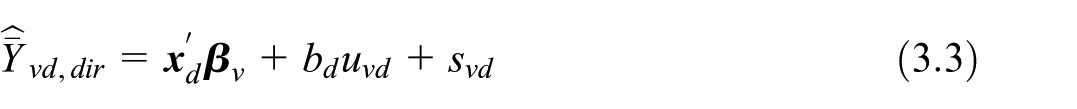
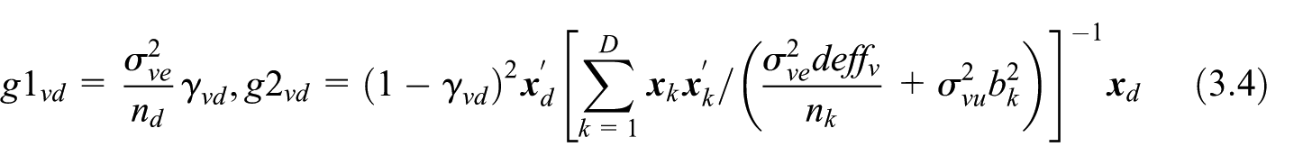
where ${\hat{\overline{Y}}}_{\mathrm{vd},\mathrm{dir}}$ is a direct estimator of $Y_{\mathrm{vd}}$ , ${\mathit{x}}_d$ are the covariates for area $U_d$ , $b_d$ is a known positive constant, $u_{\mathrm{vd}}$ and $s_{\mathrm{vd}}$ are the domain random effects and sampling errors. We have $u_{\mathrm{vd}}\begin{array}{c}\mathrm{iid}\hfill \\ \multicolumn{1}{c}{~}\\ \multicolumn{1}{c}{}\end{array}(0,{\sigma }_{\mathrm{vu}}^2)$ independent of the sampling error $s_{\mathrm{vd}}\begin{array}{c}\mathrm{iid}\hfill \\ \multicolumn{1}{c}{~}\\ \multicolumn{1}{c}{}\end{array}(0,{\psi }_{\mathrm{vd}})$ with a known variance ${\psi }_{\mathrm{vd}}$ . The BLUP of ${\overline{Y}}_{\mathrm{vd}}$ is ${\tilde{\overline{Y}}}_{\mathrm{vd}}={\mathit{x}}_d^{\prime }{\tilde{\mathit{\beta }}}_v+b_d{\tilde{u}}_{\mathrm{vd}}$ . Assuming that the variance ${\psi }_{\mathrm{vd}}$ can be modeled as ${\psi }_{\mathrm{vd}}={\sigma }_{\mathrm{ve}}^2\mathrm{def}{f}_v/n_d$ , where ${\sigma }_{\mathrm{ve}}^2$ is the variance of the random individual effects $e_{\mathrm{vi}}$ of the model in Equation (2.5) and $\mathrm{def}{f}_v$ is the design effect (Kish 1995), the components $g{1}_{\mathrm{vd}}$ and $g{2}_{\mathrm{vd}}$ of BLUP ${\tilde{\overline{Y}}}_{\mathrm{vd}}$ are:

$$g{1}_{\mathrm{vd}}=\frac{{\sigma }_{\mathrm{ve}}^2}{n_d}{\gamma }_{\mathrm{vd}},g{2}_{\mathrm{vd}}={(1-{\gamma }_{\mathrm{vd}})}^2{\mathit{x}}_d^{\prime }{[\sum _{k=1}^D{\mathit{x}}_k{\mathit{x}}_k^{\prime }/(\frac{{\sigma }_{\mathrm{ve}}^2\mathrm{def}{f}_v}{n_k}+{\sigma }_{\mathrm{vu}}^2{b}_k^2)]}^{-1}{\mathit{x}}_d$$

(3.4)

where

$${\gamma }_{\mathrm{vd}}=\frac{{\sigma }_{\mathrm{vu}}^2{b}_d^2}{({\sigma }_{\mathrm{ve}}^2\mathrm{def}{f}_v/n_d)+b_d^2{\sigma }_{\mathrm{vu}}^2}.$$

(3.5)

3.2.3. General Linear Mixed Effects Model

Equations (2.5), (3.1) and (3.3) are particular cases of the general linear mixed-effects model with a block diagonal covariance structure. We introduce this model with the symbols given in Rao (2003, Sections 6.2 and 6.3):

$${\mathit{y}}_v=\mathit{X}{\mathit{\beta }}_v+\mathit{Z}{\mathit{u}}_v+{\mathit{e}}_v,$$

(3.6)

where ${\mathit{y}}_v={({\mathit{y}}_{v1}^{\prime },\dots ,{\mathit{y}}_{\mathrm{vd}}^{\prime },\dots ,{\mathit{y}}_{\mathrm{vD}}^{\prime })}^{\prime }$ , $\mathit{X}={({\mathit{X}}_1^{\prime },\dots ,{\mathit{X}}_d^{\prime },\dots ,{\mathit{X}}_D^{\prime })}^{\prime }$ , $\mathit{Z}=\mathrm{dia}{g}_{1\le d\le D}\left({\mathit{Z}}_d\right)$ , ${\mathit{u}}_v={({\mathit{u}}_{v1}^{\prime },\dots ,{\mathit{u}}_{\mathrm{vd}}^{\prime },\dots ,{\mathit{u}}_{\mathrm{vD}}^{\prime })}^{\prime }$ , and ${\mathit{e}}_v={({\mathit{e}}_{v1}^{\prime },\dots ,{\mathit{e}}_{\mathrm{vd}}^{\prime },\dots ,{\mathit{e}}_{\mathrm{vD}}^{\prime })}^{\prime }$ , being ${\mathit{y}}_{\mathrm{vd}}=(y_{v1},\dots ,y_{\mathrm{vi}},\dots ,y_{v{N}_d}{)}^{\prime }$ , ${\mathit{X}}_d={({\mathit{x}}_1^{\prime },\dots {\mathit{x}}_i^{\prime },\dots ,{\mathit{x}}_{i{N}_d}^{\prime })}^{\prime }$ , ${\mathit{u}}_{\mathrm{vd}}={(u_{v1},\dots ,u_{\mathrm{vh}},\dots ,u_{\mathrm{vH}})}^{\prime }$ , and ${\mathit{e}}_{\mathrm{vd}}=(e_{v1},\dots ,e_{\mathrm{vi}},\dots ,e_{v{N}_d}{)}^{\prime }$ . ${\mathit{X}}_d$ and ${\mathit{Z}}_d$ are known $N_d\times p$ and $N_d\times H$ matrices of full rank, ${\mathit{u}}_v$ and ${\mathit{e}}_v$ are independently distributed with mean 0 and covariance matrices $\mathit{G}=\mathrm{dia}{g}_{1\le d\le D}\left({\mathit{G}}_d\right)$ and $\mathit{R}=\mathrm{dia}{g}_{1\le d\le D}\left({\mathit{R}}_d\right)$ depending on some variance parameters ${\mathbf{\omega }}_v={({\delta }_{v1},\dots ,{\delta }_{\mathrm{vH}})}^{\prime }$ . We suppose that ${\mathbf{\omega }}_v$ belongs to a specified subset of the Euclidean space such that $V_M\left({\mathit{y}}_v\right)=\mathrm{dia}{g}_{1\le d\le D}({\mathit{R}}_d+{\mathit{Z}}_d{\mathit{G}}_{\mathrm{vd}}{\mathit{Z}}_d^{\prime })$ , is non-singular for all ${\mathbf{\omega }}_v$ belonging to the subset. For instance, in a model that considers the correlation between different units within the same domain (D’Alò et al. 2023), ${\mathit{G}}_{\mathrm{vd}}={\mathrm{\phi }}_v{\mathbf{\Omega }}_{\mathrm{vd}}({\mathrm{\rho }}_v)$ , being ${\mathrm{\phi }}_v={\sigma }_{\mathrm{uv}}^2/{\sigma }_{\mathrm{ve}}^2$ . The structure of ${\mathbf{\Omega }}_{\mathrm{vd}}$ is known unless the variance components ${\mathrm{\phi }}_v$ and ${\mathrm{\rho }}_v$ of ${\mathbf{\omega }}_v$ . The MSE of the BLUP estimate of ${\overline{Y}}_d$ can still be expressed as the sum of the two addenda $g{1}_{\mathrm{vd}}$ and $g{2}_{\mathrm{vd}}$ in which the $g{1}_{\mathrm{vd}}$ component is a decreasing function of $n_d$ (Falorsi et al. 2023)

$$g{1}_{\mathrm{vd}}\cong \frac{{\mathrm{\sigma }}_{\mathrm{ve}}^2}{n_d}{\gamma }_{\mathrm{vd}},$$

(3.7)

where ${\gamma }_{\mathrm{vd}}$ is the $d-\mathrm{th}$ element on the main diagonal of ${\mathbf{\Gamma }}_v$ where:

$${\mathbf{\Gamma }}_v=\left[\mathrm{dia}{g}_{1\le d\le D}\left(n_d\right)\right][\mathrm{dia}{g}_{1\le d\le D}\left(n_d\right)+\mathrm{dia}{g}_{1\le d\le D}{({\mathrm{\phi }}_v{\mathbf{\Omega }}_{\mathrm{vd}}({\mathrm{\rho }}_v))}^{-1}{]}^{-1}.$$

(3.8)

As in the previous cases, $g{2}_{\mathrm{vd}}$ is a minor order term whose expression, given in still depends of the $\mathit{x}$ values of the selected sample (Falorsi et al. 2023).

3.2.4. Uncertainty on the Domain Membership Variables

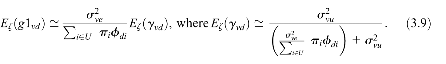
Suppose ${\lambda }_{\mathrm{di}}$ quantities are not available in the sampling frame. However, using some ${\mathit{z}}_i$ auxiliary variables, we can define a $\zeta$ model on the probability that unit $i$ belongs to the domain $U_d$ : $\mathrm{Pr}({\lambda }_{\mathrm{di}}=1\mid {\mathit{z}}_i)={\varphi }_{\mathrm{di}}$ , with $V_{\zeta }({\lambda }_{\mathrm{di}}=1\mid {\mathit{z}}_i)={\varphi }_{\mathrm{di}}(1-{\varphi }_{\mathrm{di}})$ . Assuming model independence between ${\lambda }_{\mathrm{di}}$ and $y_{\mathrm{vi}}$ , the expected value of $g{1}_{\mathrm{vd}}$ can be linearly approximated as

$$E_{\zeta }\left(g{1}_{\mathrm{vd}}\right)\cong \frac{{\sigma }_{\mathrm{ve}}^2}{\sum _{i\in U}{\pi }_i{\varphi }_{\mathrm{di}}}{E}_{\zeta }\left({\gamma }_{\mathrm{vd}}\right),\mathrm{where}{E}_{\zeta }\left({\gamma }_{\mathrm{vd}}\right)\cong \frac{{\sigma }_{\mathrm{vu}}^2}{\left(\frac{{\sigma }_{\mathrm{ve}}^2}{\sum _{i\in U}}{\pi }_i{\varphi }_{\mathrm{di}}\right)+{\sigma }_{\mathrm{vu}}^2}.$$

(3.9)

4. Sampling Optimization

4.1. The Basic Unit Level Model

4.1.1. The Optimization Problem

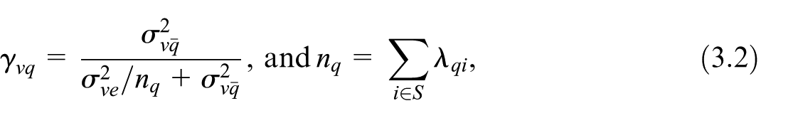
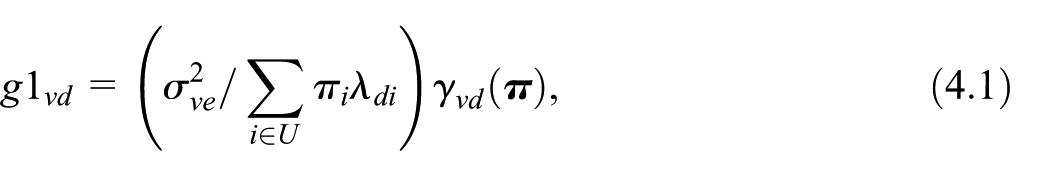
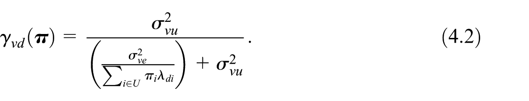
We look for the vector $\mathit{\pi }$ so as to obtain the expected minimum cost sampling design, ensuring that the terms $g{1}_{\mathrm{vd}}(v=1,\dots ,V;d=1,\dots ,D)$ are lower than pre-fixed thresholds $g{1}_{\mathrm{vd}}^{*}(v=1,\dots ,V;d=1,\dots ,D)$ . If the sample is selected with the cube method under specification in Equation (2.3) of the balancing variables, the component $g{1}_{\mathrm{vd}}$ given in Equation (2.8), can be formulated as function of the inclusion probabilities

$$g{1}_{\mathrm{vd}}=({\sigma }_{\mathrm{ve}}^2/\sum _{i\in U}{\pi }_i{\lambda }_{\mathrm{di}}){\gamma }_{\mathrm{vd}}\left(\mathit{\pi }\right),$$

(4.1)

where

$${\gamma }_{\mathrm{vd}}\left(\mathit{\pi }\right)=\frac{{\sigma }_{\mathrm{vu}}^2}{\left(\frac{{\sigma }_{\mathrm{ve}}^2}{\sum _{i\in U}{\pi }_i{\lambda }_{\mathrm{di}}}\right)+{\sigma }_{\mathrm{vu}}^2}.$$

(4.2)

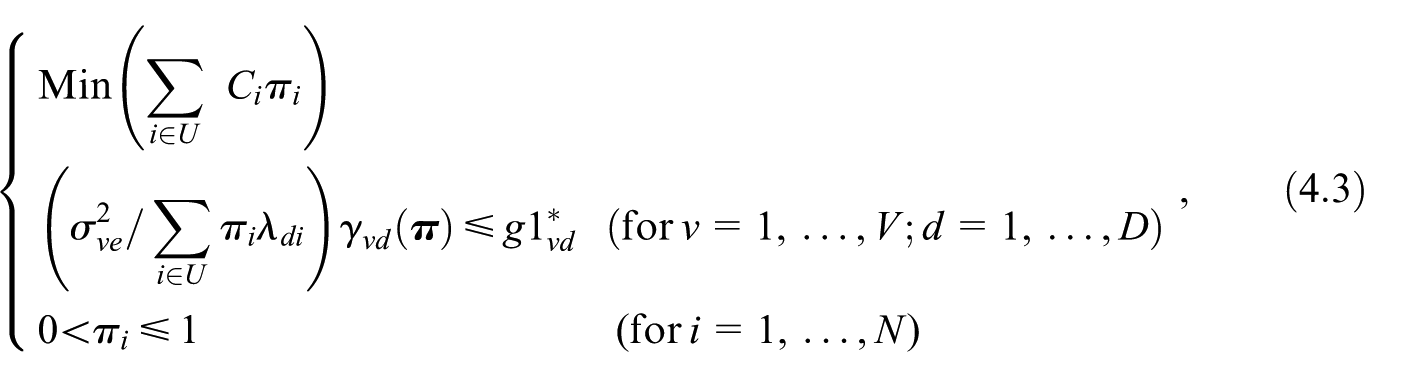
Based on Equations (4.1) and (4.2), the $\mathit{\pi }$ vector can be obtained as the solution of the following Optimization Problem (OP) based on $(V\times D)+N$ inequality constraints and with $N$ unknowns, ${\pi }_i$ :

$$\{\begin{array}{c}\mathrm{Min}\left(\sum _{i\in U}{C}_i{\pi }_i\right)\hfill \\ ({\sigma }_{\mathrm{ve}}^2/\sum _{i\in U}{\pi }_i{\lambda }_{\mathrm{di}}){\gamma }_{\mathrm{vd}}\left(\mathit{\pi }\right)\le g{1}_{\mathrm{vd}}^{*}(\mathrm{for}v=1,\dots ,V;d=1,\dots ,D)\hfill \\ 0<{\pi }_i\le 1(\mathrm{for}i=1,\dots ,N)\hfill \end{array},$$

(4.3)

where $C_i$ is the unit cost of collecting data on the $i-\mathrm{th}$ unit. The second row of OP Equation (4.3) represents the $V\times D$ constraints on the maximum values that the $g{1}_{\mathrm{vd}}$ terms can attain, and the third row identifies the $N$ constraints on the field of variation of the ${\pi }_i$ values. The variances ${\sigma }_{\mathrm{ve}}^2$ and ${\sigma }_{\mathrm{vu}}^2$ are treated as known; in practice, they must be estimated. Equation (4.3) can be solved with the fixed-point algorithm illustrated below.

4.1.2. Fixed-Point Algorithm

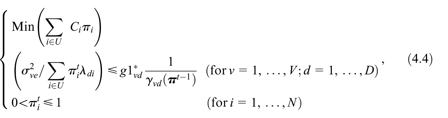
Let $t=0,1,\dots$ denote the iteration number, and let ${\mathit{\pi }}^t={({\pi }_1^t,\dots ,{\pi }_i^t,\dots ,{\pi }_N^t)}^t$ be the vector $\mathit{\pi }$ at iteration $t$ . The value of ${\gamma }_{\mathrm{vd}}$ at iteration $t$ , denoted as ${\gamma }_{\mathrm{vd}}\left({\mathit{\pi }}^t\right)$ , is calculated using Equation (4.2), by substituting the vector $\mathit{\pi }$ with ${\mathit{\pi }}^t$ .

• Step 0. Initialization. We determine the vector ${\mathit{\pi }}^0={(\pi ,\dots ,\pi ,\dots ,\pi )}^t$ where $0<\pi <1$ is a fixed scalar.

• Step 1. Calculus. At iteration $t=1,2,\dots$ , we solve the following OP

$$\{\begin{array}{c}\mathrm{Min}\left(\sum _{i\in U}{C}_i{\pi }_i\right)\hfill \\ ({\sigma }_{\mathrm{ve}}^2/\sum _{i\in U}{\pi }_i^t{\lambda }_{\mathrm{di}})\le g{1}_{\mathrm{vd}}^{*}\frac{1}{{\gamma }_{\mathrm{vd}}\left({\mathit{\pi }}^{t-1}\right)}(\mathrm{for}v=1,\dots ,V;d=1,\dots ,D)\hfill \\ 0<{\pi }_i^t\le 1(\mathrm{for}i=1,\dots ,N)\hfill \end{array},$$

(4.4)

taking the $V\times D$ values ${\gamma }_{\mathrm{vd}}\left({\mathit{\pi }}^{t-1}\right)$ as fixed. By fixing the ${\gamma }_{\mathrm{vd}}\left({\mathit{\pi }}^{t-1}\right)$ values, the objective function OP Equation (4.4) becomes a straightforward optimization problem that can be solved using standard algorithms available in software libraries for non-linear optimization (such as NLopt). The R package nloptr (https://cran.r-project.org/web/packages/nloptr/index.html) is probably a more accessible way for practitioners to use. Other two valuable options are Alabama (https://cran.rproject.org/web/packages/alabama/index.html) and the R packages CVXR (Fu et al. 2020).

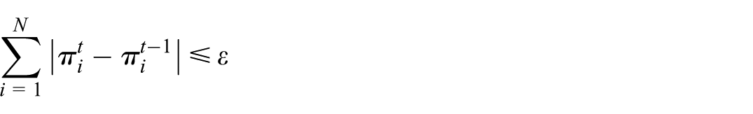
• Step 2. Fixed-point iteration. Assigning $\epsilon$ a small value (e.g., $=0.005$ ), if

$$\sum _{i=1}^N|{\pi }_i^t-{\pi }_i^{t-1}|\le \epsilon$$

the iterations stop. Otherwise, we update the values ${\gamma }_{\mathrm{vd}}\left({\pi }^{\mathrm{t}}\right)$ and iterate step 1 for $t=t+1$ , until convergence. Appendix in Falorsi et al. (2023) demonstrates that under certain approximations, the algorithm converges to a fixed-point solution for model 2.5.

4.2. Other Models

We briefly delve below into how to specify the OP and run the fixed-point algorithm for the other models illustrated in Subsection 3.2.

4.2.1. Model with Random Intercept at the Macro-Domain Level for Addressing Cases Where Budget Constraints Prevent Sample Coverage in All Small Areas: Equation (3.1)

In this case, we can control the sample size only at the macro area level. Therefore, the OP considers only $V\times Q$ constraints on the maximum values the $g{1}_{\mathrm{vq}}$ terms can take. The OP can be defined similarly to Equation (4.3) by substituting the terms ${\gamma }_{\mathrm{vq}}$ given in Equation (3.2) instead of the values ${\gamma }_{\mathrm{vd}}$ defined by Equation (2.7). The updating of the ${\gamma }_{\mathrm{vq}}\left({\mathit{\pi }}^{\mathrm{t}}\right)$ values is defined consequently.

4.2.2. Area Level Model: Equation (3.3)

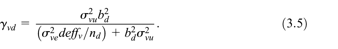
The OP is defined by Equation (4.3), where the ${\gamma }_{\mathrm{vd}}$ term is given in Equation (3.5). The fixed-point iteration is updated consequently. To run the fixed-point algorithm, the $\mathrm{def}{f}_v$ values should be known or estimated.

4.2.3. General Linear Mixed Effects Model: Equation (3.6)

The OP is defined by Equation (4.3), where the ${\gamma }_{\mathrm{vd}}$ term is the $d-\mathrm{th}$ element on the main diagonal of the matrix ${\mathbf{\Gamma }}_v$ given in Equation (3.8). The fixed-point iteration is updated consequently. To run the fixed-point algorithm, the elements of the variance vectors ${\mathbf{\omega }}_{\mathbf{v}}$ should be known or estimated.

4.2.4. Uncertainty on the Domain Membership Variables

Considering Equation (3.9), we can set the OP as

$$\{\begin{array}{c}\mathrm{Min}\left(\sum _{i\in U}{C}_i{\pi }_i\right)\hfill \\ ({\sigma }_{\mathrm{ve}}^2/\sum _{i\in U}{\pi }_i{\varphi }_{\mathrm{di}}){\gamma }_{\mathrm{vd}}\left(\mathit{\pi }\right)\le g{1}_{\mathrm{vd}}^{*}(\mathrm{for}v=1,\dots ,V;d=1,\dots ,D)\hfill \\ 0<{\pi }_i\le 1(\mathrm{for}i=1,\dots ,N)\hfill \end{array},$$

(4.5)

where ${\gamma }_{\mathrm{vd}}\left(\mathit{\pi }\right)$ is given in Equation (3.9), the probabilities ${\varphi }_{\mathrm{di}}$ are considered as known, even if they are estimated in actual situations. The specification of the corresponding fixed-point algorithm is trivial.

4.3. Some Computational Aspects

This Section briefly discusses some computational aspects, referring to Appendices A.2, A.3, and A4 for the more technical aspects.

4.3.1. Powell’s Algorithm

Powell (1994) proposed an algorithm for nonlinearly constrained optimization that can solve almost all OP illustrated in Section 3 except for Model in Equation (3.6). It is based on an iterative approach without using derivatives. The algorithm is available in the software library NLopt for non-linear optimization (http://github.com/stevengj/nlopt). In Section 5.2, we see that based on the actual data analyzed in the empirical experiment we conducted, the fixed point algorithm finds a better optimal solution than Powell’s algorithm. However, in Falorsi et al. (2023), we see that Powell’s algorithm reaches convergence faster. Moreover, the fixed-point algorithm applies to all models illustrated in Section 3.2.

4.3.2. Computational Simplification

OP Equation (4.3) is computationally complex since there are $N$ unknown ${\pi }_i$ values. We can simplify the OP by $(i)$ partitioning the population $U$ in $H$ strata such that we can obtain each domain as a union of entire strata and $(\mathrm{ii})$ defining a uniform inclusion probability at the stratum level. Under the two above conditions, we have a Stratified Simple Random Sampling Without Replacement (SSRSWOR) design. For instance, consider the case in which the domains of interest are the regions and the classes of the NACE code (https://ec.europa.eu/competition/mergers/cases/index/nace_all.html) separately. In this case, we may individuate strata by cross-classifying the modalities of the two variables region and NACE-code. Let $U_{[h]}(h=1,\dots ,H)$ be the generic stratum of $N_{[h]}$ units, where $U={\cup }_{h=1}^H{U}_{[h]}$ and $N=\sum _{h=1}^H{N}_{[h]}$ . Moreover, we have $U_d=\underset{h:{\lambda }_{d[h]}=1}{\overset{H}{\cup }}{U}_{[h]}$ , and $N_d=\sum _{h=1}^H{N}_{[h]}{\lambda }_{d[h]}$ , where ${\lambda }_{d[h]}=1$ if $U_{[h]}\in U_d$ and, ${\lambda }_{d[h]}=0$ otherwise. We use square brackets to denote strata in the introduced notation to avoid confusing domains with strata. We assign a uniform inclusion probability to units in stratum $U_{[h]}$ , ${\pi }_i=n_{[h]}/N_{[h]}$ for $i\in U_{[h]}$ , where $n_{[h]}$ is the sample size of stratum $U_{[h]}$ . With a SSRSWOR design, since $H<<N$ , we can define an OP (see Appendix A2), which is computationally much more straightforward than OP Equation (4.3) because it considers only $H$ unknown values that are the proportions $n_{[h]}/N_{[h]}$ .

4.3.3. OP That Considers HT Estimates in Larger Domains and SAE Estimates in Smaller Domains

Let us consider the case where there are larger domains in which sample estimates are calculated using the HT estimator. At the same time, we use model-based estimates for smaller domains. Let us illustrate this case for the SSRSWOR design just introduced to avoid too many complexities. Furthermore, suppose we can define the strata, such as each domain (large or small) can be obtained by aggregating entire strata. Let $U_{\ell }$ $(\ell =1,\dots ,L)$ be a large domain, where $U_{\ell }=\underset{h:{\lambda }_{\ell [h]}=1}{\overset{H}{\cup }}{U}_{[h]}$ , and $N_{\ell }=\sum _{h=1}^H{N}_{[h]}{\lambda }_{\ell [h]}$ , where ${\lambda }_{\ell [h]}=1$ if $U_{[h]}\in U_{\ell }$ and, ${\lambda }_{\ell [h]}=0$ otherwise. The same notation holds for all the small domains $U_d$ . In this setting, as illustrated in Appendix A3, we can define an OP that finds the minimum cost solution guaranteeing the accuracy for both the large and small domains, where the accuracy for the small domains is based on the model. In contrast, the large domain’s accuracy is defined in terms of the sampling variance of the HT estimator.

4.3.4. Including the Term g2 in the Optimization

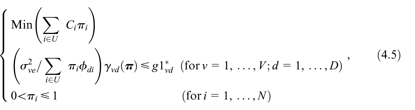
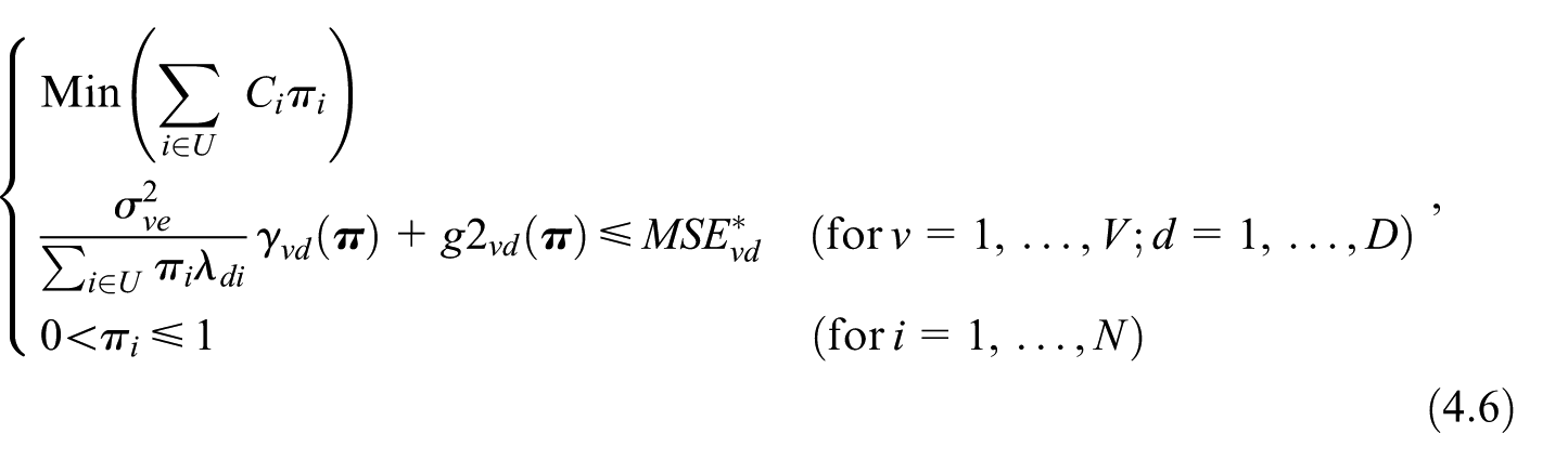
Suppose the sample is selected using the Cube algorithm, with the balancing variables defined by Equation (2.4). In this case, the sample selection ensures that the following two conditions are met, at least approximately $\sum _{i\in S}{\lambda }_{\mathrm{di}}=n_d,\mathrm{and}{\overline{\mathit{X}}}_d\cong {\overline{\mathit{X}}}_{\mathrm{ds}}$ . Hence, $g{2}_{\mathrm{vd}}$ may by defined as a function of the vector $\mathit{\pi }$ , as $g{2}_{\mathrm{vd}}\left(\mathit{\pi }\right)={\left[{\overline{\mathit{X}}}_d(1-{\gamma }_{\mathrm{vd}}\left(\mathit{\pi }\right))\right]}^{\prime }$ ${\sigma }_{\mathrm{ve}}^2{\mathit{A}}_v^{-1}\left[{\overline{\mathit{X}}}_d(1-{\gamma }_{\mathrm{vd}}\left(\mathit{\pi }\right))\right]$ . We can include the term $g{2}_{\mathrm{vd}}$ in the optimization by defining the following OP

$$\{\begin{array}{c}\mathrm{Min}\left(\sum _{i\in U}{C}_i{\pi }_i\right)\hfill \\ \frac{{\sigma }_{\mathrm{ve}}^2}{\sum _{i\in U}{\pi }_i{\lambda }_{\mathrm{di}}}{\gamma }_{\mathrm{vd}}\left(\mathit{\pi }\right)+g{2}_{\mathrm{vd}}\left(\mathit{\pi }\right)\le {\mathrm{MSE}}_{\mathrm{vd}}^{*}(\mathrm{for}v=1,\dots ,V;d=1,\dots ,D)\hfill \\ 0<{\pi }_i\le 1(\mathrm{for}i=1,\dots ,N)\hfill \end{array},$$

(4.6)

As illustrated in Appendix A4, OP Equation (4.6) can be solved under some approximations with an algorithm based on two nested fixed-point iterations.

4.3.5. Two-Stage Sampling

OP Equation (4.3) can be easily extended to other sampling designs. We illustrate here the case of a two-stage design. Let $U$ be a population of $N$ clusters. In order to avoid introducing too many new symbols, the index $i$ will be used to denote the cluster rather than the generic unit. The $i-\mathrm{th}$ cluster has $M_i$ final units. Suppose that the probability of belonging to $U_d$ is quite uniform for the ultimate sampling units of the cluster and approximately equal to ${\varphi }_{\mathrm{di}}$ . A first-stage sample, $S$ , of size $n$ is selected without replacement from $U$ , with varying inclusion probabilities $\mathit{\pi }$ . Suppose the cluster $i-\mathrm{th}$ is included in the sample $S$ . In that case, a fixed number, $m_i$ , final units are selected without replacement and with equal probabilities out of the $M_i$ , final units of the cluster. Under Equation (2.5), we can define $g{1}_{\mathrm{vd}}={\sigma }_{\mathrm{ve}}^2{\gamma }_{\mathrm{vd}}{\left(\sum _{i\in U}{\pi }_i{m}_i{\lambda }_{\mathrm{di}}\right)}^{-1}$ where ${\gamma }_{\mathrm{vd}}={\sigma }_{\mathrm{vu}}^2{[({\sigma }_{\mathrm{vu}}^2/\sum _{i\in U}{\pi }_i{m}_i{\lambda }_{\mathrm{di}})+{\sigma }_{\mathrm{vu}}^2]}^{-1}$ . The objective function of the OP is $\mathrm{Min}\left(\sum _{i\in U}{C}_i{m}_i{\pi }_i\right).$ This type of sampling design is commonly used in household surveys conducted by national statistical offices, such as those carried out by ISTAT (the Italian National Institute of Statistics). Typically, a two-stage design is applied within strata that group primary sampling units according to geographical domains. When the inclusion probabilities of the first-order units are approximately proportional to the size of the population, this sampling design ensures final inclusion probabilities for all the final sampling units within the stratum, which leads to optimality properties as it significantly reduces the variability of the final sampling weights.

5. Experimental Study

The proposed methodology underwent rigorous testing on both simulated data generated by a superpopulation model and actual open data from a survey conducted by the ISTAT.

In addition to the nature of data generation, the two experiments differ significantly. In the first experiment, we examined one continuous variable where there is a relatively high value of the variance ${\sigma }_{\mathrm{vu}}^2$ of the domain effects $u_d$ . In the second experiment, we examined the case of a multidimensional variable where the variances ${\sigma }_{\mathrm{vu}}^2$ have a relatively slight impact.

Considering a model-generated population allowed us to control the various factors influencing the results. On the other hand, actual data examination revealed some weaker results.

Both experiments unequivocally underscore the paramount importance of a well-defined sampling design in enhancing the accuracy of SAE estimates. This key finding not only validates our research but also amplifies its relevance in the field.

Cadamuro (2023) conducted other experimental studies using synthetic open data derived from the Australian Agricultural and Grazing Industries Survey that are congruent with those given in this section and confirms the relevance of the sampling design when producing small area estimates.

A reader of the following Section 5 might be somewhat confused as to why different data are used and why the same outputs are not applied across examples. It is worth noting that in both experiments—on simulated and real data—we followed the same methodological steps; however, when presenting the results, we chose to emphasize the aspects most relevant for the reader.

5.1. Simulatated Population

5.1.1. Data Generation

Let $U$ be a population of size $N=10,000$ . Let $U_d(d=1,\dots ,D=100)$ be a small domain of interest, where the set of the 100 domains defines a partition of the population. We first randomly assign the 10,000 units to the D domains. Furthermore, let $U_q(q=1,\dots ,Q=10)$ be a large domain. We assumed the first ten small domains form the first large domain, the following ten the second large domain and so on.

We generated a single response variable, $y_{\mathrm{vi}}$ , for the finite population $U$ , according to the model

$$y_{\mathrm{vi}}={\beta }_v{x}_i+u_{\mathrm{vq}}+u_{\mathrm{vd}}+{ϵ}_{\mathrm{vi}}\mathrm{for}i\in U_q\cap U_d$$

(5.1)

where $x~N(10,{\sigma }_x^2),u_{\mathrm{vq}}~N(0,{\sigma }_{\widehat{\mathrm{vq}}}^2),u_{\mathrm{vd}}~N(0,{\sigma }_{\mathrm{vu}}^2)$ , and ${ϵ}_{\mathrm{vi}}~N(0,1)$ , in which $x_i$ , $u_{\mathrm{vq}}$ $u_{\mathrm{vd}}$ , and ${ϵ}_{\mathrm{vi}}$ are independent of one another. Variances are fixed as ${\sigma }_x^2=7/4,{\sigma }_{\widehat{\mathrm{vq}}}^2=3,{\sigma }_{\mathrm{vu}}^2=3$ , and $\beta =2.2$ . In the experimental setup, several parameter sets were evaluated, and the configuration that most clearly produced the scenario with a relatively high variance ${\sigma }_{\mathrm{vu}}^2$ of the domain effects $u_{\mathrm{vd}}$ was retained. Although other configurations yielded comparable outcomes, this choice was made to ensure clarity and conciseness in the exposition.

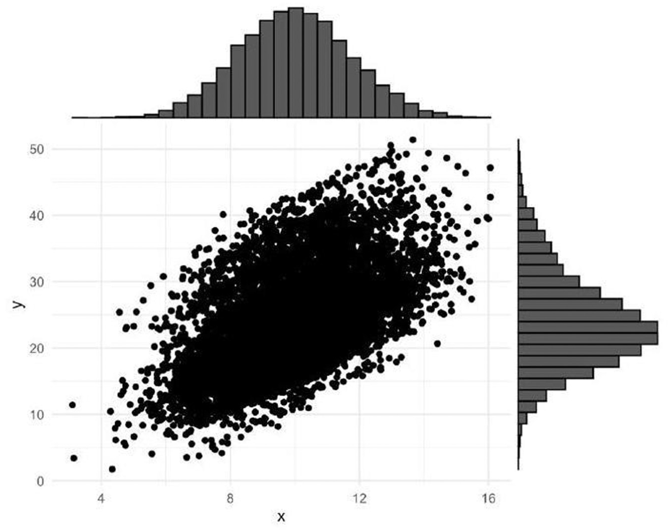
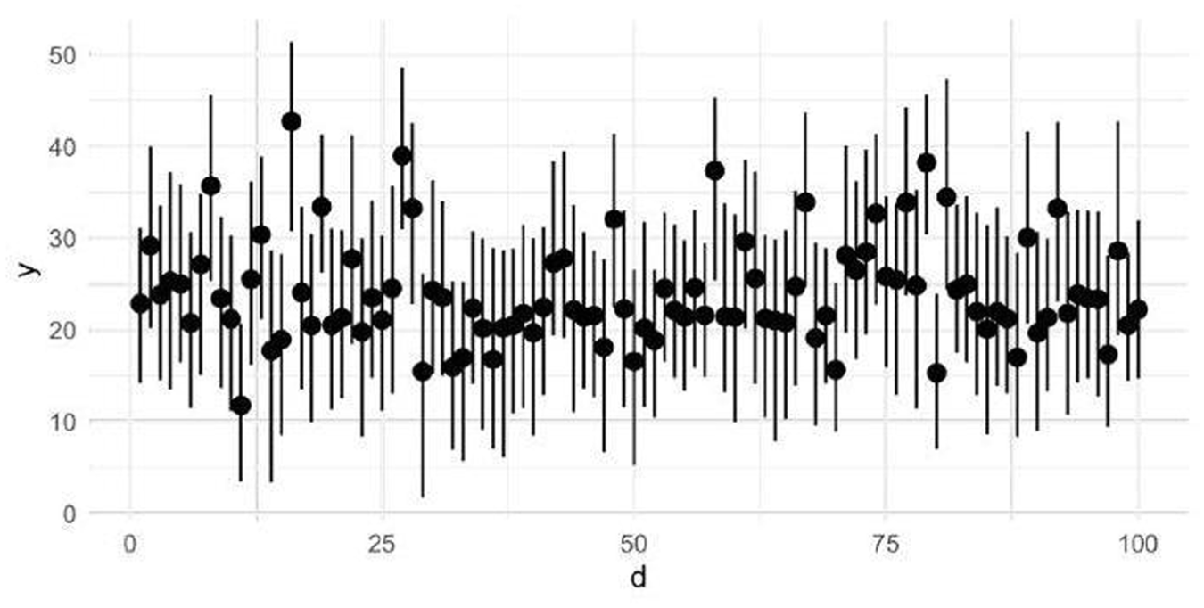
We first generated the 110 random area values $u_d(d=1,\dots ,D=100)$ and $u_q(q=1,\dots ,Q=10)$ . Then for each unit $i$ , we generated the 10,000 $e_{\mathrm{vi}}$ and $x_i$ random values. The final values $y_{\mathrm{vi}}$ are then obtained by adding the fixed value ${\beta }_v{x}_i$ and the random components $e_{\mathrm{vi}}$ , $u_{\mathrm{vq}}$ , and $u_{\mathrm{vd}}$ . The joint density of the overall generated data has a normal distribution (Figure 1). The $D=100$ domains have different population sizes and variability of the target variable as shown in Figure 2.

Figure 1.

Joint density distribution of generated data.

Figure 2.

Min-max range of the generated data by domains.

5.1.2. The Sample Allocation

We have a budget for a maximum of 150 interviews, which means we can expect to conduct 1.5 interviews per domain. To determine our sampling strategy, we will use a small area indirect estimator based on the following working model:

$$y_{\mathrm{vi}}={\beta }_v{x}_i+u_{\mathrm{vd}}+e_{\mathrm{vi}},$$

(5.2)

where with reference to the model in Equation (5.1), we have $e_{\mathrm{vi}}=u_{\mathrm{vq}}+{ϵ}_{\mathrm{vi}}$ . The model in Equation (5.2) is simpler than the model in Equation (5.1) which generated the population data. This case reflects a realistic situation for the sampling design stage where the knowledge one has about the data is only approximate.

We performed the sampling allocation based on the computational simplification illustrated in Subsection 4.3.2. We partioned the population $U$ in $H=D=100$ strata such that each small domain $U_d$ corresponds to a stratum $U_{[h]}$ . Moreover, we defined a uniform inclusion probability and a uniform cost at the stratum level. To render expressive the variance threshold, we defined them as relative errors given by ${\mathrm{RE}}_{\mathrm{vd}}^{*}=\sqrt{g{1}_{\mathrm{vd}}^{*}}/{\overline{Y}}_{\mathrm{vd}}$ . We tune the ${\mathrm{RE}}_{\mathrm{vd}}^{*}$ values equal to 0.035 in all areas, thus achieving an overall sample size of 144 units. Even if the threshold ${\mathrm{RE}}_{\mathrm{vd}}^{*}$ , defined in relative terms, is fixed as equal in all the domains, the threshold $g{1}_{\mathrm{vd}}^{*}$ defined in terms of totals, varies among the domains since increasing the ${\overline{Y}}_{\mathrm{vd}}$ values, the $g{1}_{\mathrm{vd}}^{*}$ has to grow as well to fix the relative error $g{1}_{\mathrm{vd}}^{*}$ . In our experiment the totals ${\overline{Y}}_{\mathrm{vd}}$ are known. In actual applications, ${\overline{Y}}_{\mathrm{vd}}$ is unknown. Therefore, if we want to define the error threshold in relative terms, we must replace ${\overline{Y}}_{\mathrm{vd}}$ in the relative error threshold with an estimated value (for instance, from a previous survey). From now on, we denote this allocation as opt.

We compared the opt sample allocation and the Proportional to the Population Size Allocation (PPSA) method. The latter is the expected allocation in a sampling strategy using a Simple Random Sampling Without Replacement (SRSWOR) design.

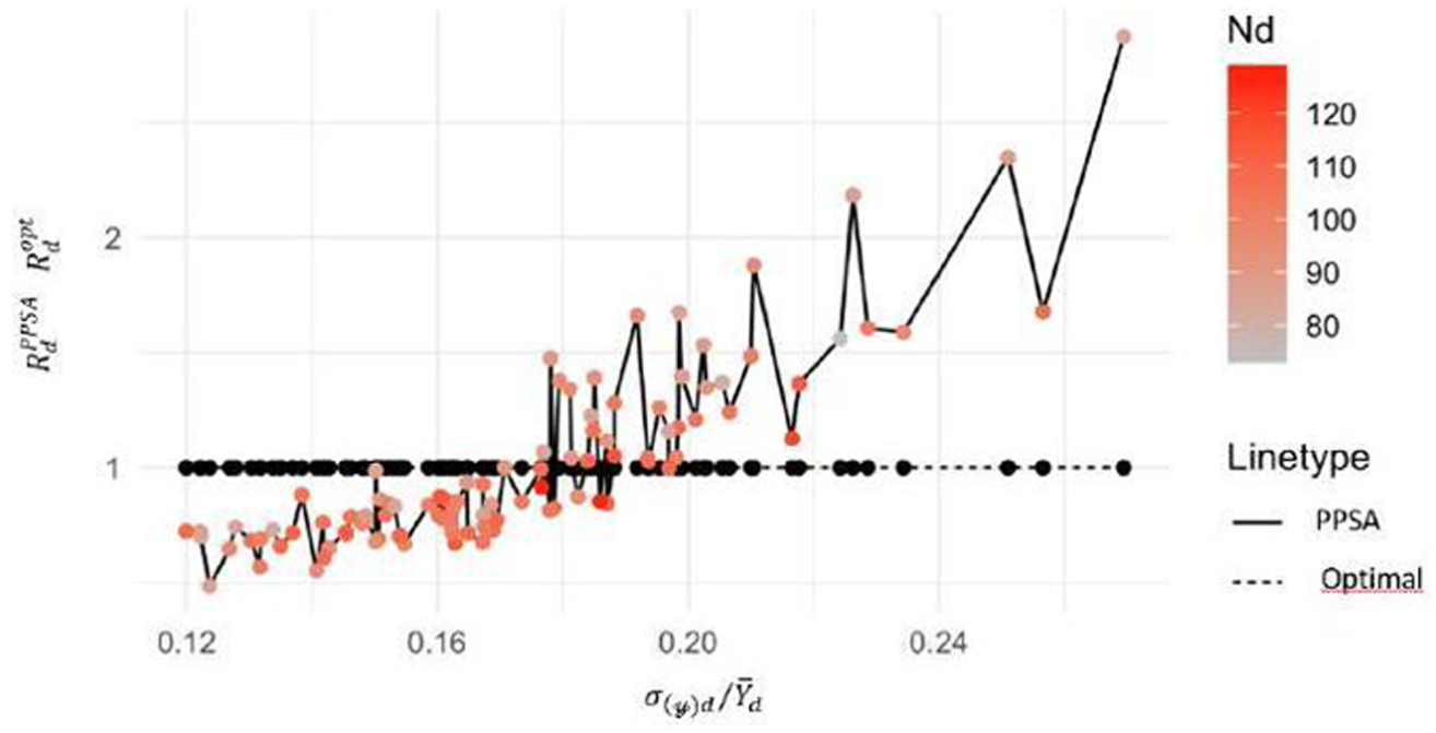
Figure 3 shows the expected sampling error for the 100 domains for the fixed population generated, as illustrated in Subsection 5.1.1. The horizontal axis considers the Coefficient of Variation $\left(C{V}_d\right)$ of the actual domain $y$ values, where $V_d=$ ${\sigma }_d/{\overline{Y}}_d$ , being ${\sigma }_d^2=\sum _{i\in U_d}{(y_i-{\overline{Y}}_d)}^2/N_d$ . The vertical axis shows the ratio $R_d^{\alpha }=g{1}_d^{\alpha }/g{1}_d^{*}$ between the value of g1, calculated according to the $\alpha$ allocation (with $\alpha =\mathrm{opt}$ and PPSA) and the threshold value $g{1}_d^{*}$ . A value of $R_d^{\alpha }$ of 1 means that exactly the sample required to achieve the desired accuracy $g{1}_d^{*}$ is allocated to the domain. Conversely, a value less than 1 means too much of the sample is allocated to the domain concerning the desired precision. If the value is greater than 1, it indicates that the sample allocated is not sufficient to achieve the desired precision. In such cases, more sample units should be allocated in the domain. It can be observed that the ratio $R_d^{\mathrm{opt}}$ of the opt solution is always 1 for every domain, which is an expected outcome. If there is only one target variable $y$ and there are $D$ non-overlapping domains, then the $D$ constraints on the terms of $g{1}_{(v)d}$ of OP are satisfied by equality. Falorsi et al. (2023) have illustrated another experimental situation where the study domains intersect. In that experiment, the opt allocation always leads to solutions where many $R_d^{\mathrm{opt}}$ values are lower than 1, which ensures the constraints on accuracy. However, in some domains, the values of the ratio $R_d^{\mathrm{opt}}$ are equal to 1, while other domains need to be oversampled to guarantee the desired accuracy.

Figure 3.

Domain ratios $R_d^{\mathrm{PPSA}}$ and $R_d^{\mathrm{opt}}$ versus ${\sigma }_{(y)d}/{\overline{\mathrm{Y}}}_d$ domain values.

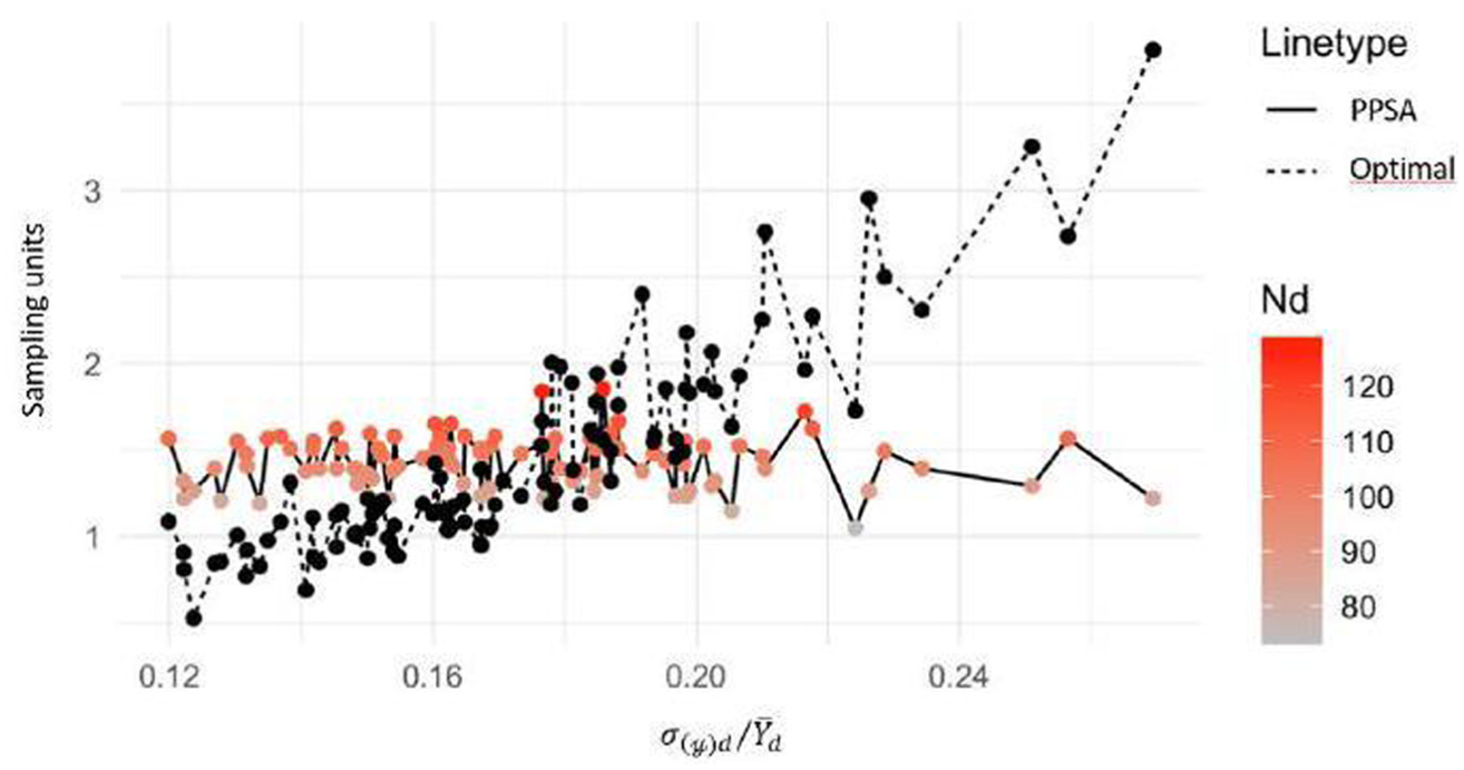
In contrast, the ratio $R_d^{\mathrm{PPSA}}$ values of the PPSA allocation show that the values are larger or smaller than 1. We note that two elements affect the domain estimates’ variance: the coefficient of variation of the actual domain $y$ values ( $C{V}_d)$ and the population size. The PPSA does not consider the domain $C{V}_d$ , so with larger $C{V}_d$ , we have a more significant sampling error with a given sample size. This issue is well depicted in Figure 3 by the increasing trend of the graph of $R_d^{\mathrm{PPSA}}$ . The domain population size explains the irregularities of the trend. Two domains with similar $C{V}_d$ but different population sizes have different expected sampling errors since the PPSA gives a number of sample units proportional to the size. Large domains have smaller sampling errors. The color of the dots in the PPSA graph shows the different population sizes. Optimal allocation is a compromise solution between the one driven by domain size and that derived from variability expressed in $C{V}_d$ . It gives more sampling units when ${\sigma }_{(y)d}/{\overline{Y}}_d$ and/or $N_d$ , as shown in Figure 4.

Figure 4.

Sampling units of optimal and PPSA allocations versus ${\sigma }_{(y)d}/{\overline{\mathrm{Y}}}_d$ domain values.

5.1.3. Monte Carlo Simulation

Here, we compared the expected variances with the empirical variance achieved through a Monte Carlo simulation. We generated 1,000 samples from the fixed population illustrated in Subsection 5.1.1. While the population values remain fixed, the different Monte Carlo samples $S_d^r(r=1,\dots ,1,000;d=1,\dots ,D)$ differ in the subset of $n_d$ elementary units $(i=1,\dots ,n_d)$ selected in the sample. For each replication $r$ of a given sampling allocation $\alpha$ , we calculated the domain EBLUP estimates ${\hat{\overline{Y}}}_d^{\alpha ,r}$ . We compared the accuracy of the SAE estimates considering three different sampling designs:

1. the stratified simple random sampling design (from now on denoted as Stratified) where the sample sizes in strata are given by rounding up the opt solution;

2. the stratified balanced random sampling design (from now on denoted as Balanced) with the sample allocation equal to that of the stratified design, but where the sampling selection was carried out balancing the $x$ values at the domain level;

3. the SRSWOR design which represents the sampling design adopted when we do not consider the small areas in the design. We use this as the benchmarking sampling strategy.

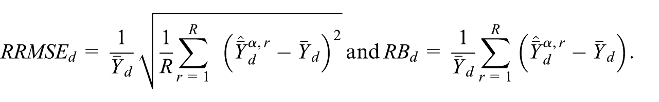
The discussion of the results presented below is essentially based on two leading indicators, the Relative Root Mean Square Error (RRMSE) and Relative Bias (RB) defined as

$$\mathrm{RRMS}{E}_d=\frac{1}{{\overline{Y}}_d}\sqrt{\frac{1}{R}\sum _{r=1}^R{({\hat{\overline{Y}}}_d^{\alpha ,r}-{\overline{Y}}_d)}^2}\mathrm{and}R{B}_d=\frac{1}{{\overline{Y}}_d}\sum _{r=1}^R({\hat{\overline{Y}}}_d^{\alpha ,r}-{\overline{Y}}_d).$$

5.1.4. Results

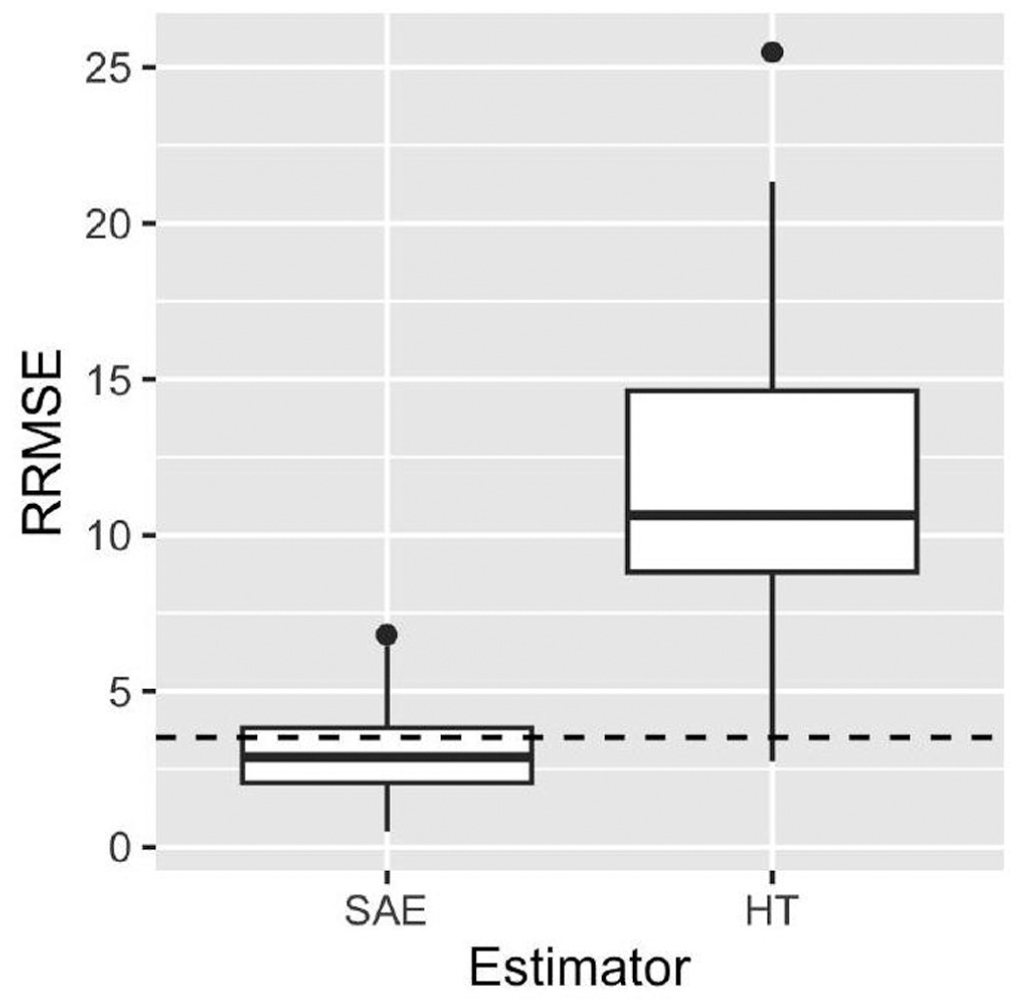
Figure 5 shows the Relative RRMSE of the eblup SAE and HT estimator using the Balanced sampling design. The SAE is the best choice in our experimental setting. The same results that were not presented in this paper arise using the stratified and SRSWOR sampling design.

Figure 5.

RRMSE of the eblup SAE and Horvitz-Thompson estimator $(\mathit{HT})$ using the Balanced sampling design.

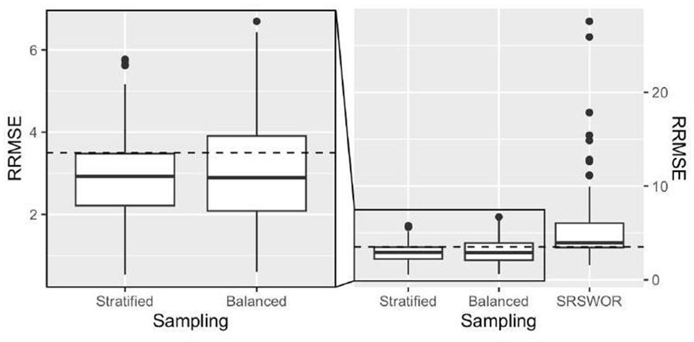
Focusing on the three different sampling designs and SAE, Figure 6 shows that the Stratified and Balanced design produced a smaller Monte Carlo RRMSE for the 100 domains compared to the SRSWOR design. The RRMSE is larger than expected in some Stratified and Balanced design domains. This evidence can be explained because the allocation method neglects the $g{2}_d$ term. Furthermore, the EBLUP estimator is applied in the simulation, while the BLUP estimator is considered during the sampling allocation phase. This aspect can affect the observed empirical results. It is possible to observe empirical domain MSEs larger than the correspondent planned ones due to the relative impact of terms $g_2$ and $g_3$ for each domain $g_2$ and $g_3$ for each domain $d(d=1,\dots ,D)$ .

Figure 6.

RRMSE of the eblup SAE estimator under different sampling designs.

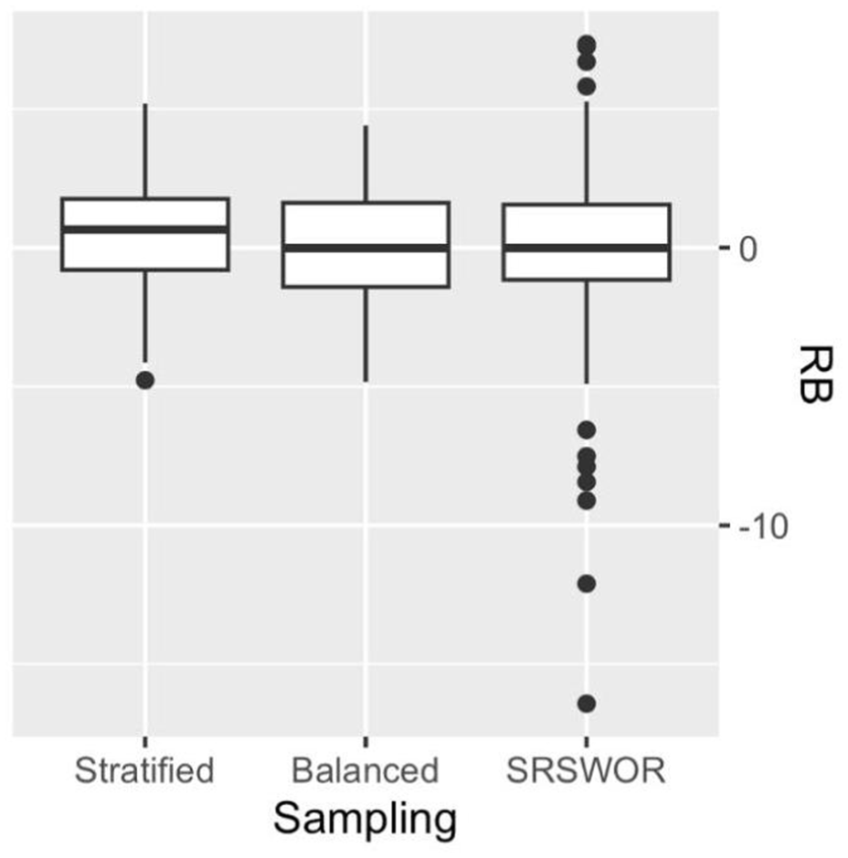
Finally, we compared the three sampling strategies based on their RB. The results for the 100 domains are presented in Figure 7. The Balanced strategy yielded estimates with smaller RB, making it the most effective. The expected RB value was negligible for both the Balanced and SRSWOR strategies, while it was slightly positive for the Stratified design. The SRSWOR strategy produced extremely large positive and negative RB values, making the Stratified or Balanced designs preferable alternatives.

Figure 7.

RB of eblup SAE estimator under different sampling designs.

5.2. Real Data

5.2.1. Data Description

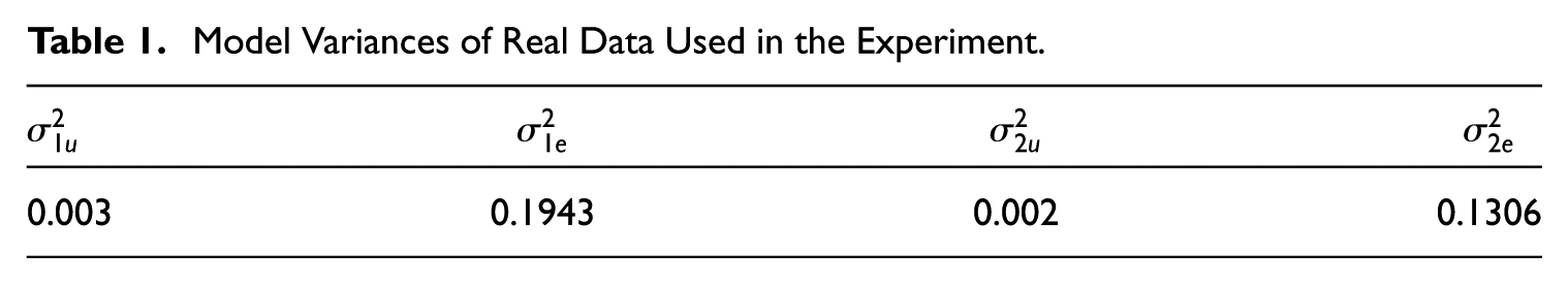
We tested the proposed approach on synthetic public data consisting of 10,000 individuals and 104 municipalities, available in the link provided in parenthesis (https://www.istat.it/microdati/rilevazione-sulle-forze-di-lavoro-dati-trasversali-trimestrali-file-per-la-ricerca/), derived from the Labor Force Sampling Survey by the Italian National Institute of Statistics. These data are provided to users to assist them in using the R package MIND (D’Alò et al. 2023) to implement multivariate models for small areas. After some data cleaning, we considered the target population as a subset of those data, consisting of 9,152 individuals and 92 municipalities. The small areas $U_d$ of our experiment are the 92 municipalities resulting after data cleaning. The ${\mathit{x}}_i$ variables for individual $i$ are: Sex by age class (14 categories), Educational level (six levels), Nationality (1 = Italian, 2 = otherwise), Municipality code (92 codes). We have two binary target variables $y_{\mathrm{vi}}$ describing the employment status where: $y_{1i}=1$ if the person is seeking employment and $y_{1i}=0$ , otherwise; $y_{2i}=1$ if the person is employed and $y_{2i}=0$ otherwise. Using these data, we applied model 2.5, obtaining the values of model variability shown in Table 1. Model 2.5 is highly predictive for employment but weaker for job seekers.

Table 1.

Model Variances of Real Data Used in the Experiment.

${\sigma }_{1u}^2$	${\sigma }_{1e}^2$	${\sigma }_{2u}^2$	${\sigma }_{2e}^2$
0.003	0.1943	0.002	0.1306

5.2.2. Sampling Allocation

We conducted the sampling allocation based on the computational simplification illustrated in Subsection 4.3.2. We partitioned the population $U$ in $H=D=92$ strata such that each small domain $U_d$ corresponds to a stratum $U_{[h]}$ . Moreover, we define a uniform inclusion probability and a uniform cost at the stratum level.

The allocation strategy was mainly focused on controlling the model error of the number of people seeking employment. This variable is considered the most challenging one for estimation, as it occurs less frequently, and the models used for estimation have lower predictive power. However, we also kept the error of SAE estimates relating to employed individuals under control.

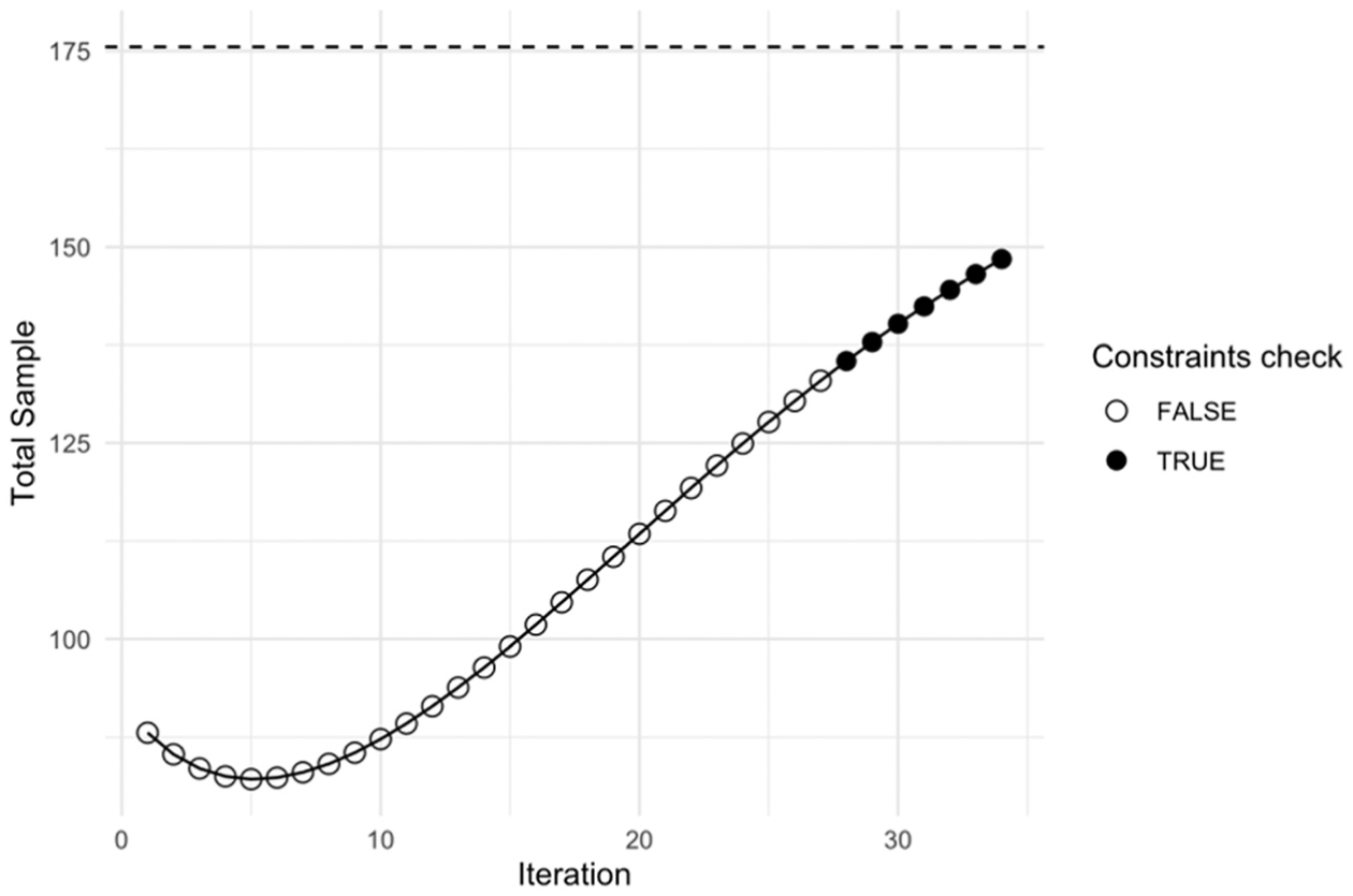
As in the case of simulated data, in this exercise we assumed a sufficient budget for around 150 interviews. To find a sampling solution compatible with this budget, we defined the OP benchmarks (expressed in relative error ${\mathrm{RE}}_{\mathrm{vd}}^{*}=\sqrt{g{1}_{\mathrm{vd}}^{*}}/{\overline{Y}}_{\mathrm{vd}}$ ) with values around 0.25 for people looking for work and 0.126 for employed people. Regarding the variable ${\mathrm{y}}_v$ , it was not feasible to establish a single ${\mathrm{RE}}_{\mathrm{vd}}^{*}$ value for all domains, unlike in the simulated data. This was because, in certain domains, the average ${\overline{Y}}_{\mathrm{vd}}$ value was too low, resulting in a very small benchmark variance $g{1}_{\mathrm{vd}}^{*}$ . This would have absorbed a disproportionately large sample in those domains, making it difficult to define an equal ${\mathrm{RE}}_{\mathrm{vd}}^{*}$ value across all domains. We ran the fixed-point algorithm and obtained a solution of approximately 136 units in total based on the given constraints. We denote this allocation as “opt.” The algorithm’s search path is displayed in Figure 8, where the dark circles represent the solutions that meet the constraints. As seen in the figure, the algorithm checks for local optima even after finding the optimal solution. The additional black points appearing after the optimal solution has been reached are due to an early stop mechanism in the algorithm. This mechanism halts the iterations after a certain number to prevent the risk of converging to a local minimum. The dashed line on the figure, around 175 units, represents the solution given by Powell’s algorithm, which converges faster but finds a less efficient solution (see Subsection 4.3.1).

Figure 8.

The Search path of the optimal solution (opt) of the Fixed-point algorithm.

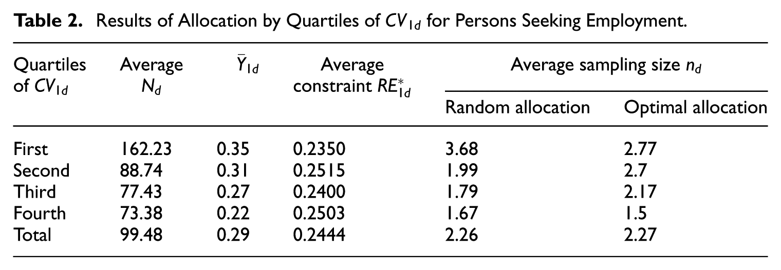
To explain the allocation process, we first calculate the coefficient of variation $\left(C{V}_{\mathrm{vd}}\right)$ of the actual domain $y_v$ values, where $V_{\mathrm{vd}}=$ ${\sigma }_{\mathrm{vd}}/{\overline{Y}}_{\mathrm{vd}}$ , being ${\sigma }_{\mathrm{vd}}^2=\sum _{i\in U_d}{(y_{\mathrm{vi}}-{\overline{Y}}_{\mathrm{vd}})}^2/N_d$ . For each variable $y_v$ , we then classified the domains into quartiles based on their $C{V}_{\mathrm{vd}}$ Tables 2 and 3 display the opt allocation results for job seekers and employed individuals, respectively, for each quartile. We compared these results with those of a random allocation, which, on average, allocates the sample into domains proportionally to their size in terms of units.

Table 2.

Results of Allocation by Quartiles of $C{V}_{1d}$ for Persons Seeking Employment.

Quartiles of $C{V}_{1d}$	Average $N_d$	${\overline{Y}}_{1d}$	Average constraint ${\mathrm{RE}}_{1d}^{*}$	Average sampling size $n_d$
				$\mathrm{Random}$ allocation	Optimal allocation
First	162.23	0.35	0.2350	3.68	2.77
Second	88.74	0.31	0.2515	1.99	2.7
Third	77.43	0.27	0.2400	1.79	2.17
Fourth	73.38	0.22	0.2503	1.67	1.5
Total	99.48	0.29	0.2444	2.26	2.27

Table 3.

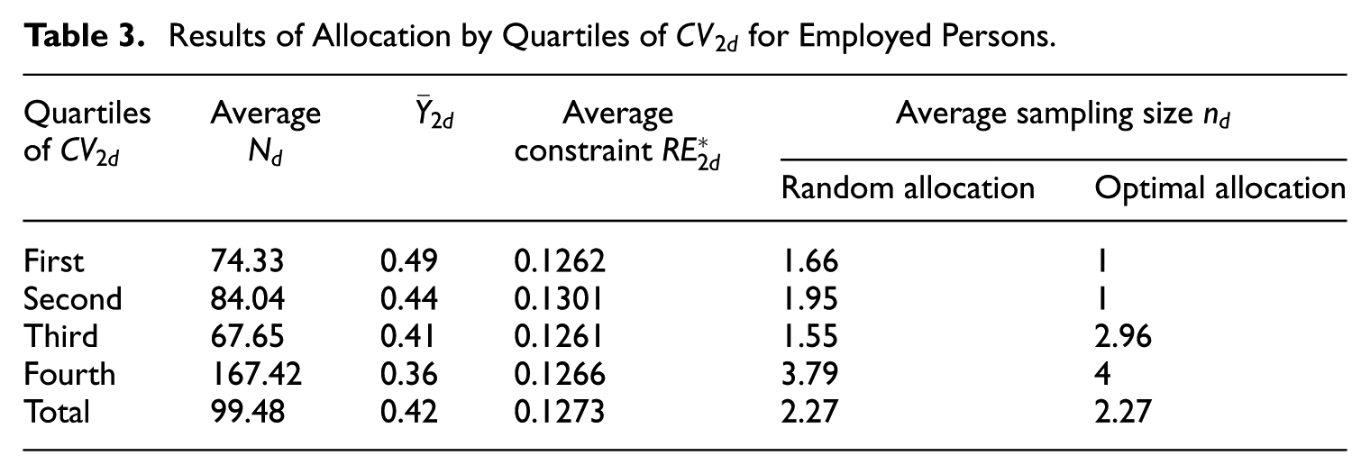
Results of Allocation by Quartiles of $C{V}_{2d}$ for Employed Persons.

Quartiles of $C{V}_{2d}$	Average $N_d$	${\overline{Y}}_{2d}$	Average constraint ${\mathrm{RE}}_{2d}^{*}$	Average sampling size $n_d$
				$\mathrm{Random}$ allocation	Optimal allocation
First	74.33	0.49	0.1262	1.66	1
Second	84.04	0.44	0.1301	1.95	1
Third	67.65	0.41	0.1261	1.55	2.96
Fourth	167.42	0.36	0.1266	3.79	4
Total	99.48	0.42	0.1273	2.27	2.27

When it comes to the variable of individuals seeking employment, we observed that optimal allocation yields a more balanced distribution compared to random allocation. Random allocation tends to concentrate the sample in areas with higher population, whereas optimal allocation distributes the sample away from those regions and assigns it to areas that pose more difficulties. In the fourth quartile, however, the two allocations are approximately equivalent. This effect may be due to the need to ensure an error benchmark also for the estimate of employed people. Upon analyzing the employment estimate, we noticed that the third quartile of the distribution tends to be oversized. This could be due to the impact of other variables. The optimal allocation finds an efficient compromise between the requirements defined for the two variables.

The evidence from the last two columns of Tables 2 and 3 highlights that the planned accuracy ( ${\mathrm{RE}}_{\mathrm{vd}}^{*}$  = 0.25 for job seekers and 0.126 for employed individuals) can be attained with as little as one observation per domain.

5.2.3. Monte Carlo Simulation

From the population illustrated in Subsection 5.2.1, we selected 1,000 samples for each of the two allocations considered, and we constructed the EBLUP estimates. We also calculated the Horvitz-Thompson estimates for each sample selection of the random allocation. We then calculated the $\mathrm{RRMS}{E}_{\mathrm{vd}}$ and $R{B}_{\mathrm{vd}}$ indicators similarly to what was illustrated in Subsection 5.1.3. We present the results only for the variable “people seeking occupation” because there are no substantial differences between the two sample allocations for the other variable, which is undoubtedly due to the predictive goodness of the SAE model for this latter variable.

5.2.4. Results

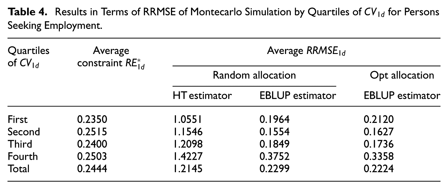
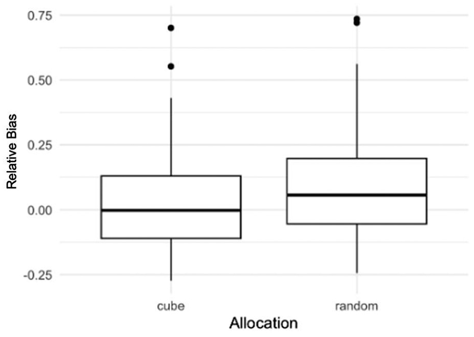
Table 4 illustrates the RRMSE results from Monte Carlo simulations by quartiles of $C{V}_{1d}$ for persons seeking employment. For domains above the median of the quartile distribution (i.e., those with higher difficulty), the EBLUP estimator under optimal allocation consistently achieves a lower RRMSE values compared to random allocation. This highlights the advantage of optimal allocation in reducing errors in problematic domains, which are characterized by higher variances and lower means. In contrast, for domains below the median of the quartile distribution (i.e., those with lower difficulty), the RRMSE values for both allocation strategies are approximately equivalent, with a slight preference for random allocation. However, these domains are not problematic, as they already provide accurate estimates regardless of the allocation method. In summary, we emphasize that our approach is a compromise. The key advantage of our proposed sampling method, in contrast to a standard one, is its ability to optimally allocate samples across various domains. This strategy helps us minimize excessively high errors in certain areas while only slightly increasing errors in domains where the SAE estimates are already accurate. This trade-off underscores the overall benefit of the optimal allocation strategy compared to random allocation. We further note that in the last quartile group, both methods fail to fully comply with the constraints. However, the RRMSE of the EBLUP estimate under optimal allocation is closer to the constraint. This non-compliance likely arises because the optimization assumes the absence of model estimation bias, which, in this case, is introduced by extreme values in the data (refer to Figure 9). Nevertheless, the scatter plots in Figure 9 indicate that the optimal allocation offers better protection against bias, further supporting its effectiveness in challenging scenarios.

Table 4.

Results in Terms of RRMSE of Montecarlo Simulation by Quartiles of $C{V}_{1d}$ for Persons Seeking Employment.

Quartiles of $C{V}_{1d}$	Average constraint ${\mathrm{RE}}_{1d}^{*}$	Average $\mathrm{RRMS}{E}_{1d}$
		Random allocation		Opt allocation
		HT estimator	EBLUP estimator	EBLUP estimator
First	0.2350	1.0551	0.1964	0.2120
Second	0.2515	1.1546	0.1554	0.1627
Third	0.2400	1.2098	0.1849	0.1736
Fourth	0.2503	1.4227	0.3752	0.3358
Total	0.2444	1.2145	0.2299	0.2224

Figure 9.

The relative bias $(R{B}_{1d})$ of EBLUP estimators for the two allocations.

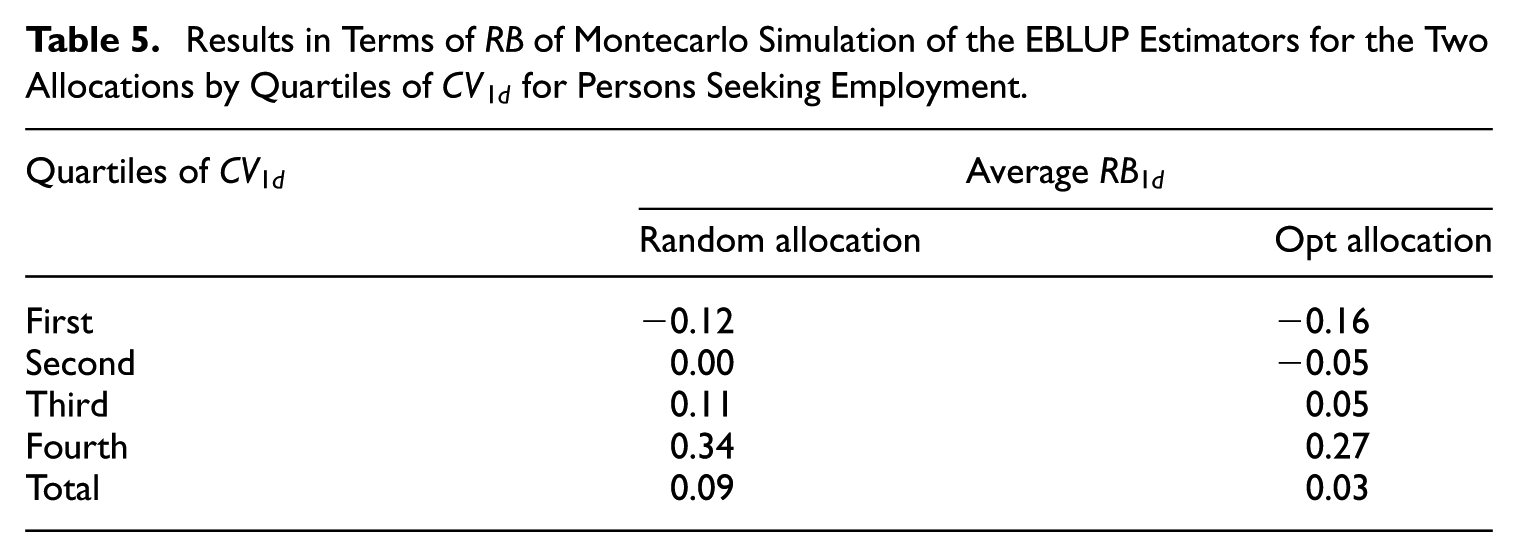
Finally, Table 5 illustrates the bias of EBLUP estimators for the two allocations. The relative bias of the opt allocation for the most problematic areas (i.e., those above the median) is lower.

Table 5.

Results in Terms of $\mathrm{RB}$ of Montecarlo Simulation of the EBLUP Estimators for the Two Allocations by Quartiles of $C{V}_{1d}$ for Persons Seeking Employment.

Quartiles of $C{V}_{1d}$	Average $R{B}_{1d}$
	Random allocation	Opt allocation
First	−0.12	−0.16
Second	0.00	−0.05
Third	0.11	0.05
Fourth	0.34	0.27
Total	0.09	0.03

6. Conclusions

Developing an overall strategy to address the Small Area Estimation (SAE) problem remains an unsolved issue in the finite population inference. Usually, the SAE strategy focuses on the specific estimation techniques, moving the sampling design to the background. This paper has delved into how a carefully designed sampling design allows us to improve the accuracy of SAE estimates, at least in cases where small domains of interest can be identified at the sampling design stage.

The strategy we propose is based on three steps. First, we define a working SAE model for the small areas of interest. This model must be simple since sampled units have not yet been observed. Furthermore, the model must align with the overall available budget. Essentially, this means that the levels of the random factors defined in the model should not exceed the overall sample size permitted by the survey budget. In this way, we can select a sample where the various random components are predicted by direct observation and do not solely rely on the synthetic part of the estimator. The proposed working model must be a compromise between a complex model that accurately describes reality and a simplified model that nevertheless allows the fundamental random components to be kept under control.

Then, we defined a non-standard optimization method for defining the vector of inclusion probabilities in order to minimize the expected minimum cost sampling design, by ensuring that the model-based estimates respect the desired model-based accuracy. This optimization problem aims for an efficient allocation of the sample units in the estimation domains. We also studied the algorithmic solutions necessary to solve the optimization problem.

The third pillar of the strategy is based on sample selection. We suggest a balanced sample selection technique that allows to control the sample size for each of the random effects defined in the model and, if possible, to control the mean value of the auxiliary variables involved in the fixed part of the working model.

Experiments on a simulated data sets showed that controlling sampling sizes is crucial for small domains to protect against inaccurate model-based estimations and to ensure that the accuracy level never exceeds the established accuracy. In the experiments, strategies that neglect the sampling design exhibit highly heterogeneous sampling errors among the domains, with some domains receiving few or none sample units and others many more than needed.

It is worth noting that while our approach focuses on optimizing inclusion probabilities to guarantee cost-effective accuracy for small area estimation, the method of penalized balanced sampling proposed by Breidt and Chauvet (2012) enhances efficiency by modifying the cube method through penalization. The two strategies, therefore, differ in perspective: our solution ensures accuracy through planned allocation, whereas theirs emphasizes design-based efficiency via penalization, offering complementary but distinct pathways.

Future research on this topic will cover several aspects. In our view, the first point to be addressed is the one sketched in Appendix A3 for a simplified statistical setting, where an optimality condition is sought, considering that estimates for larger domains can be obtained with estimators (such as HT) that are unbiased concerning the sampling design. In contrast, those for smaller domains are obtained with model-based estimators. Other aspects that need to be addressed in more detail, both theoretically and in terms of application, are related to SAE models useful in situations where the overall survey budget only allows direct observation in some small areas. Such cases may represent considerable interest in many SAE real situations where the estimation domains are too small to control their sampling sizes in the design phase.