
Abstract
Significant enhancements have been made in small area estimation (SAE) methodology because there has been an increased demand for reliable estimates through SAE over the past decades. This article describes the advanced statistical methodology used to produce state and county model-based estimates of average scores and various proficiency levels of adults for all states and counties, using data from the first cycle of the US Program for the International Assessment of Adult Competencies and the American Community Survey. Challenges and issues are discussed especially in light of the small number of sample counties with survey data. Each major stage of the estimation process is discussed, including the approach for generating design-based survey estimates and modelled variances, identifying a set of predictor variables (available and measured consistently for all counties), the hierarchical Bayes linear threefold models, including bivariate models for proportions, and the diagnostics and evaluation.
Introduction
To make evidence-based policies and laws relating to adult education, sound research is needed using reliable data that are most relevant to the jurisdiction, for example, the state or county in the United States. The Program for the International Assessment of Adult Competencies (PIAAC) is an international study under the leadership of the Organization for Economic Co-operation Development. The first cycle of PIAAC involved over 30 countries and was designed to provide national estimates of the proficiency of adult literacy, numeracy, and problem-solving skills. Because the US PIAAC sample size was too small to support state and county estimates, the small area estimation (SAE) methodology was used to produce model-based estimates of average scores for literacy and numeracy, and various proficiency levels of adults of 16-74 years old residing in the United States in 2012-2017.
The term SAE refers to a variety of methods or statistical techniques to estimate parameters for subpopulations or smaller domains of interest. In the past decades, two major types of SAE models have been developed: area- and unit-level models. Area-level models take as input survey direct estimates and auxiliary data at the area level. 1 The unit-level models take as input survey data and auxiliary data at the unit level. 2 An overview of theoretical developments and a number of notable implementations have been provided. 3 The review covers topics particularly important for the application to be described here. One of these topics is the possible effect of an informative sample design on estimating the SAE model.4, 5 Another topic is the extension to multivariate models. 6 The Fay-Herriot model has been extended to estimate correlated descriptive measures. 7 They found that the multivariate empirical best linear unbiased predictors (EBLUPs) have a lower mean square error (MSE) than the corresponding EBLUPs from univariate models when the true generating model is multivariate. A bivariate hierarchical Bayes (HB) SAE model has been developed 8 using sparse survey data available for fine domains defined by geography, occupations, work levels within occupations, and job characteristics from the Bureau of Labor Statistics' National Compensation Survey. This model accounts for a more general variancecovariance structure for the latent effects. Also, the model is used to predict employee compensation in a large number of domains without survey data.
In terms of applications to literacy proficiency estimates, state- and county-level estimates of the proportions of adults lacking basic prose literacy skills were produced by the National Center for Education Statistics (NCES) using data from the 2003 National Assessment of Adult Literacy (NAAL) and 1992 National Adult Literacy Survey (NALS), 9 and model-based SAE methods. The estimates were constructed using an HB unmatched area-level twofold model using 2003 NAAL and auxiliary data from the 2000 census. 10 The model consisted of two "unmatched" components of the approach: a normal sampling model for the county-level direct survey estimates of the percentages and a smoothing (or linking) model to link the logit of the true, underlying, percentages to a set of auxiliary variables that were available, measured consistently for all counties, and related to the outcome. The model was "twofold" in that the smoothing model included random effects for the states and counties. The process was repeated using the 1992 NALS data. In addition, model-based SAE methods were applied to literacy assessment data. 11 The authors were faced with a continuous variable that had a large peak of zero values, which can happen in developing countries where zero value indicates illiteracy and positive values measure the level of literacy. In the United Kingdom, a unit-level nonlinear (logistic) model was used for literacy and numeracy binomial outcomes for the 2011 Skills for Life Survey. 12 A modeldependent approach was developed using Canadian PIAAC data. 13 The author used population parameters derived from the survey data and auxiliary information, such as census to produce provincelevel estimates of skill distribution. Netherlands' PIAAC data were used 14 to produce municipality-level average literacy scores using a unit-level linear HB model, and an area-level linear model was used to model the proportion of low literates.
In our application of SAE, which was sponsored by NCES with an extensive background discussion, 15 county-level HB linear threefold models (i.e., using random effects for counties, states and census divisions) are developed using PIAAC data. The models are used to predict four outcomes of interest for adult literacy and numeracy proficiencies for counties (the small area for this study) that are in the sample and counties that are out of the sample: an average score (on the PIAAC scale of 0-500), and the proportion of adults at or below Level 1 (low proficiency), at Level 2 (medium proficiency) and at or above Level 3 (high proficiency). There were challenges to overcome in the application of the SAE methodology to US PIAAC, which include the existence of small sample size within counties and a small proportion of the US counties with the sample, existence of the sampling error and imputation error, and the aggregation of county-level predictions.
A description of the sources of data is provided in the ‘Background on Ingested Data’ section, including PIAAC and data from other sources. In the ‘Description of the PIAAC Small Area Estimation Process’ section, methodology is discussed including a covariate selection process to gather strong covariates, predictions through a bivariate model and conducting extensive model diagnostics. To allow major sources of error to propagate through the modelling process into the resulting estimates, a hierarchical modelling framework is used. A threefold model brings the model-based estimates into close alignment with the design-based estimates at high levels of aggregation. Next, the results for each step in the process are presented in the ‘Results’ section. The last section contains a summary of the findings, supplemented by the discussion of the dissemination of the model-based estimates.
Background on Ingested Data: Sources and Key Issues
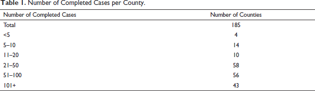
PIAAC is the sixth of a series of adult skills surveys, sponsored by NCES, which have been implemented in the United States. The first cycle of PIAAC included three national data collections (in 2012, 2014 and 2017). In each year, a four-stage stratified area probability sample was selected. In the first stage, primary sampling units (PSUs) were selected with probabilities proportionate to size, consisting of individual counties or groups of contiguous counties. In the second stage, secondary sampling units (SSUs) were selected, consisting of census blocks (e.g., a city block bounded by streets) or block groups (generally contains between 600 and 3,000 people). Dwelling units were selected in the third stage where a screener interview was used to identify the eligible persons. Using a computer-assisted personal interviewing system, in the fourth stage, one or more eligible persons were selected. Next, a Background Questionnaire (BQ) interview was administered, and then respondents were provided with the assessment. To increase the number of counties with PIAAC data for the SAE modelling process, the 2012, 2014 and 2017 samples were combined resulting in 12,330 respondents from 185 counties. Sample weights were created for the combined PIAAC 2012/2014/2017 sample for the purpose of survey estimates. Response rates ranged from 70% in 2012 to 56% in 2017. The US PIAAC Technical Report 16 provides more sample design details.
Key Issues Inherent in the Ingested Data from PIAAC
The first key issue inherent in the PIAAC data that presents challenges from the modelling perspective is informative sampling and nonresponse. PSUs were selected with probability proportionate to size sampling, and therefore the set of states and counties with the PIAAC sample results from informative sampling, which needs to be addressed in the SAE process. Also, when nonresponse is not sufficiently explained by the weighting variables used in weighting adjustments, informative nonresponse exists. In particular, literacy-related nonresponse needs to be addressed, which is estimated to be about 5% of the population. Due to a literacy-related reason (language barrier, reading/writing barrier or mental disability), such nonrespondents cannot complete the BQ and assessment (conducted in English). Cases that received a final weight include respondents to the BQ and literacy-related nonrespondents; however, the BQ literacy-related nonrespondents did not receive a literacy score.
A second issue inherent in the PIAAC data is related to the small sample sizes within counties and a small number of counties with sample. Table 1 provides a breakdown of the county sample sizes for the combined 2012/2014/2017 sample. Of the 50 states, plus the District of Columbia, 44 have completed cases in the combined 2012/2014/2017 sample. In addition, only about 6% of the counties in the United States (185 out of 3,142) have PIAAC respondent data.
Number of Completed Cases per County.
A third key issue is the existence of the sampling error (due to small sample sizes within counties) and the imputation error. The imputation error exists due to the PIAAC test design, which is based on an approach most common to the major large-scale assessments. To reduce respondent burden, a subset of test items is administered such that different groups of respondents answer different sets of items. For each domain, scores are derived using item response theory (IRT) scaling. A total of 10 plausible values (PVs, or multiple imputations) help to facilitate a measure of the uncertainty of the cognitive measurement. In a population model, the PVs are drawn from a posterior distribution based on the IRT scaling of the cognitive items with a latent regression model using information from the BQ. For more details about the IRT scaling models and the population models, see chapter 17 of the OECD PIAAC Technical Report. 17
Predictor Variables
Model-based SAE methods are used to produce estimates for areas where survey data are insufficient for reliable design-based estimation. The SAE models ‘borrow strength’ across related counties and from the auxiliary information to produce reliable model-based estimates. Model-based SAE estimates for counties that are not part of the national sample would rely almost entirely on the model, since designbased estimates are not available for such counties. That is, the model structure and covariates play an important role in the prediction of county levels of proficiency for literacy or numeracy. Reliable data sources and variables to serve as potential covariates of proficiency levels were initially identified, and more than 70 county-level variables across five major variable types were obtained as potential predictors from eight data sources. Focus was given to variables that were found to be related to the adult literacy skills in previous studies,18, 19 and were available for all the counties in the nation. These variables included those related to location, education, demographic characteristics, socio-economic status and immigration status. In addition to county-level variables, a set of 24 state-level variables was selected to provide additional information. These variables included those related to socio-economic status and education such as the graduation rate.
Description of the PIAAC SAE Process
The general method steps include creating the model inputs (including the selection of covariates), developing the model, generating predictions for all counties in the nation, aggregating predictions to the state and national levels, and performing diagnostics and evaluations.
Creating the Model Inputs
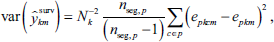
For the model inputs, the methods include computing design-based estimates and variances, making adjustments using survey regression estimation (SRE) and conducting variance smoothing. Designbased estimates were computed for each of the 185 counties for the outcomes of interest, where informative nonresponse is addressed, in which it is assumed that any literacy-related nonresponse is below Level 1 (which impacts the estimation of the proportion at or below Level 1), and for the estimation of averages, the first percentile of proficiency scores is imputed for literacy-related nonrespondents.
The multiple imputation variance estimate
20
is used to account for both the sampling error and the imputation error in the PIAAC estimates. First, the survey estimate for the mth PV for county k is computed as

where
Next, SRE was used to help address small sample sizes and concerns about resulting large variances and the representation of the sample within each county with a sample. The survey regression estimate of the mth PV for county k can be written in the following form
22
:

where Age groups: 18-19; 20-24; 25-34; 35-44; 45-54; 55-64 and 65-74 years Gender by age: males of age 18-74 years Race/ethnicity by age: Black of age 18-74 years and Hispanic of age 18-74 years Educational attainment by age: less than high school education of age 18-64 years, high school education of age 18-64 years, college education of age 18-64 years and bachelor’s degree of age 18-64 years Nativity by age: foreign born of age 20-74 years.
It is necessary for the predictors for the unit-level SRE model to have (a) population totals that had the same definition and coverage as the corresponding PIAAC variables (obtained from the American Community Survey [ACS] 2012-2016) and (b) have a low level of item nonresponse (less than 5%) where imputation was used to fill in the missing values. The approach brought survey-estimated county population totals closer to the county totals from a reliable external source.
In SAE, the use of SRE and the Taylor series variance estimation approach is described.
3
, pp. 21-23 For each PV, the SRE variance was estimated by applying the standard variance expression to the residuals (e
l
), with PSUs as strata and SSUs as clusters. Each county is in a single stratum (PSU), which simplifies the notation. Counties with only one sample segment were excluded in the following computation of the sampling variance for each PV:
where
The HB models (to be discussed) for the PIAAC SAE process assume that the variances of the SRE county estimates are known, whereas in practice they are estimated as

where 
where
Selecting Covariates for the SAE Models
Only 185 counties have PIAAC data, and therefore the model-based estimates will rely on the model extensively for a vast majority of the counties in the United States. To improve the strength of the SAE models, an extensive covariate selection process has been developed with a hope that predictors can be found that are highly related to the key outcomes. A summary of the process is discussed here, while more details can be found in Ren et al. 23 First, the candidate predictor variables are treated as fixed effects and a correlation matrix is created among all the covariates to identify highly correlated variables. One variable in each of the highly correlated pairs is dropped to avoid multicollinearity. Then the least absolute selection and shrinkage operator (LASSO) method 24 is used to select several sets of covariates for each of the four outcome models for literacy and for numeracy. To taking into account the random effect estimation in the SAE model (described below), the final list of covariates is determined using a cross-validation process. Note that the probability of selection of the PSUs is included in the variable selection process to help address informative sampling; however, it did not enter the final model.
Developing the Model and Conducting Diagnostics
An SAE modelling approach is used to produce model-based estimates that are the predictions of how the adults in a state or county would have performed had they been administered the PIAAC assessment. The methodology uses PIAAC survey data in combination with ACS data at the county level to model the quantities of interest.
Models for Proportions
In terms of producing estimated proportions of literacy and numeracy proficiency and continuing to address the propagation of high levels of the sampling error and the imputation error, an area level bivariate HB linear threefold model is developed. The model is fitted at the county level, with the input data being the sets of county-level survey regression estimates and their associated variance estimates (smoothed). Modelled jointly are two proportions: Level 1 and below and Level 3 and above. Through subtraction, the third proportion (Level 2) is derived. The model is written using a hierarchical form, that is, a linking-level accounts for the relationship between the target proportions and the covariates, and a sampling level is used for the direct estimates of proportions. A linear relationship between the proportions and the predictors is assumed for the linking model, which has random effects at three nested levels defined by the county, state and census division. To account for multiple outcomes, the SAE model is specified using the matrix form notation as follows:

where
Using the hierarchical model specification, sources of error are accounted for, including: smoothed sampling variances and random effects at the county, state and division levels. A benefit of the threefold model is that model-based estimates for counties and states without a sample will not be fully synthetic because they will be functions of direct estimates in other counties and states. Another benefit is that associations of counties within states, and states within census divisions will be accounted for, helping improve precision of the modelbased estimates at all these three levels of aggregation. In doing so, benchmarking 1 the estimates may not be necessary. The Bayesian approach is used for inference, and prior distributions are adopted for the model parameters. Summaries for the model-based estimates, such as credible intervals, and functions of the model parameters, such as the Level 2 proportion are straightforward through the use of Bayesian methods.
Independent priors are assumed for the regression coefficients and the random effects in the fully specified HB model. Specifically, it is assumed 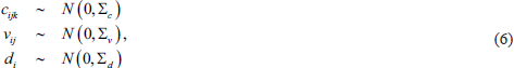
where 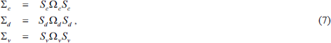
where
Models for Averages
For each domain, PIAAC averages were estimated using an area-level univariate HB linear threefold model, which includes three levels of random effects: county, state and census division. The model is specified as follows:

where 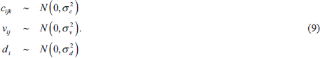
For the random effects, the variances
Model Fitting, Estimation and Prediction
Using the PIAAC sample data available in 184 counties with at least 2 records, the proportion and average models are fitted to literacy and numeracy data separately. RStan, the R interface to the Stan modelling language, is employed for this purpose. The R and Stan starting seeds used in the generation of sequences of random numbers are set equal to constants so that results can be repeated.
Markov chain Monte Carlo (MCMC) methods are used for the HB models. Three independent Markov chains are run to facilitate the calculation of Monte Carlo standard errors.26, 27, p. 229 The modelfitting procedure starts with three assigned sets of distinct initial values for
Across the 4,500 MCMC samples, predictions are produced for proportions and averages of sampled counties, non-sampled counties (without PIAAC data) and for states and nations. The posterior mean 
The values of
Aggregation to the State Level and the National Level
Once the county model-based estimates are produced, the estimates for states (and the nation) are computed as weighted aggregates county estimates for each iteration, where the weights represent the total of the county household population of adults ages 16-74 years, obtained from the 2013-2017 ACS data.
Diagnostics
The models were subjected to rigorous diagnostic checks that included various methods of internal and external model validation. The methods of internal model validation included convergence and mixing diagnostics, collinearity tests, residual analysis, posterior predictive checks, model sensitivity checks, examining changes in the specification of the prior distribution for the variance-covariance matrices (including changes in initial values and in hyperparameters values), examining changes in the model specification including univariate versus bivariate models for literacy proportions, tuning parameters in the Hamiltonian Monte Carlo and no-U-turn sampler algorithms and relaxed normality assumptions in the bivariate HB models for proportions.
The methods of external model validation included examining histograms of differences between model-based and survey estimates, shrinkage plots, interval coverage plots, bubble plots of survey regression estimates and model-based estimates, and smoothed and small area model variances, as well as comparing aggregates of model predictions and survey estimates. The model results were also assessed on the merits of improvements in precision.
Results
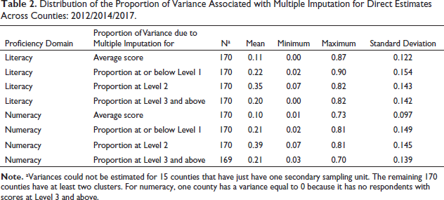
As shown by Table 2, at the county level, the imputation error can be a significant portion of the variance and cannot be ignored when producing variance estimates. For literacy skills, imputation contributes on average 11% of total variance for the average score, 22% of total variance for the proportion at or below Level 1,35% of total variance for the proportion at Level 2 and 20% of total variance for the proportion at Level 3 and above. Across counties, the contribution to the total variance from multiple imputation ranges from nearly 0% to 90%. The distribution of the proportion for numeracy is similar to that for literacy. The results clearly show that the survey estimates and variance estimates must properly use the PVs.
Distribution of the Proportion of Variance Associated with Multiple Imputation for Direct Estimates Across Counties: 2012/2014/2017.
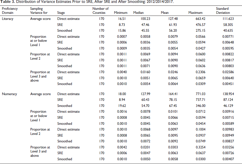
In Table 3, for averages, the proportion at or below Level 1 and that at Level 3 and above, the median SRE variance is shown to decrease substantially in comparison to the variance associated with the corresponding direct estimates. However, for the proportion at Level 2, there is only a modest decline. The R2 for the Level 2 models are of the order 0.04 compared with 0.27 for the Level 1 or below models, 0.25 for the Level 3 and above models, and 0.40 for averages. Also, from the table, one can see the impact from the variance smoothing process. While the level of variance is essentially maintained as shown by the median, the standard deviation of the variance is lower for the smoothed variance than for the SRE variance, as expected.
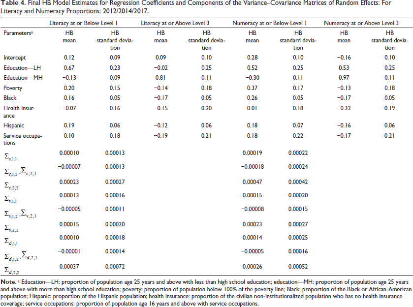
Related to covariate selection, the PSU selection probability was initially included as a potential county-level covariate to account for the informative sampling design; however, it is not identified as a significant predictor through the covariate selection process. Covariates with the highest correlations are education related; for example, the correlation is greater than 0.7 for the proportion of population with lower than high school education versus proportion at or below Level 1 literacy. Reducing the large pool of variables through the use of correlations arrived at the following initial covariates selected at the county level: percentage of population age 25 years and above with less than high school education (no high school diploma), percentage of population age 25 years and above with more than high school education (including some college, no degree), percentage of population below 100% of the poverty line, percentage of Black or African-American population, percentage of Hispanic population, percentage of civilian noninstitutionalized population who has no health insurance coverage, percentage of population age 16 years and above with service occupations, percentage of foreign-born people who entered the United States after year 2010 among the population born outside the United States, percentage of population born outside of the United States, percentage population age 16 years and above who did not work at home who spend more than 60 minutes to travel to work, unemployment rate, percentage of diabetes diagnosed, the birth rate per 1,000 women, and the average amount of grant and scholarship aid received. During the cross-validation phase of the variable selection process, a decision was made to use the same set of seven county-level variables from the 2013 to 2017 ACS data in all four models fitted for proportions and averages for literacy and numeracy. The seven covariates provide strong models for proportions and averages. For example, the adjusted R2 is 0.58 for the linear regression of literacy proportions at or below Level 1 on the seven covariates. More details on the results for each step of the covariate selection process are published. 23 The estimated model parameters are given in Table 4 for the bivariate models for proportions and in Table 5 for the univariate models for averages.
Distribution of Variance Estimates Prior to SRE, After SRE and After Smoothing: 2012/2014/2017
Final HB Model Estimates for Regression Coefficients and Components of the Variance–Covariance Matrices of Random Effects: For Literacy and Numeracy Proportions: 2012/2014/2017
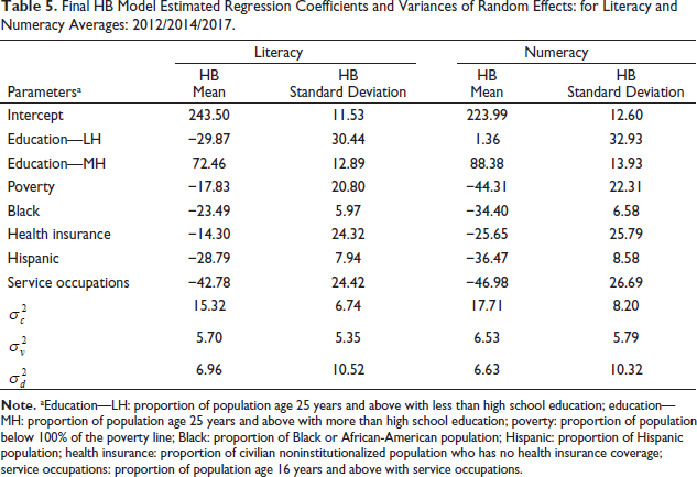
Final HB Model Estimated Regression Coefficients and Variances of Random Effects: for Literacy and Numeracy Averages: 2012/2014/2017.
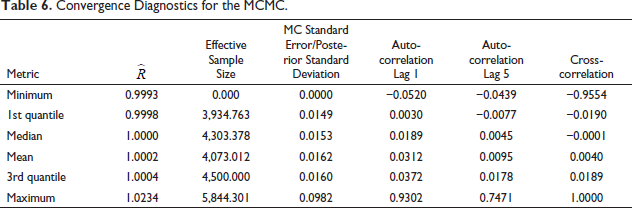
In Table 6, the mean and quartiles of diagnostic statistics are shown, including the effective sample size, Gelman-Rubin
Convergence Diagnostics for the MCMC.
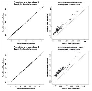
To determine the benefits from using the bivariate model, the proportions using univariate models are modelled with uniform priors on the variances, on a wide range, 0-1.000,. and compared against the bivariate model with LKJ on the correlation matrix (specification one in the report) and half-Cauchy on the standard deviations. Figure 2 illustrates the results for these comparisons for county-level literacy proportions under univariate and bivariate HB models, respectively. When the proportions are modelled using a bivariate model, the posterior variances are reduced as expected.
In Figure 1, the top row relates to proportions at or below Level 1 and the bottom row relates to proportions at or above Level 3. The left-hand side illustrates the relationship between the posterior means, while the right-hand side displays the relationship between the posterior standard deviations.
Posterior Means and Standard Deviations for County-Level Literacy Proportions Under Univariate and Bivariate HB Models: 2012/2014/2017.
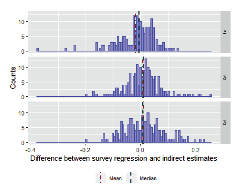
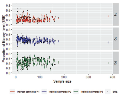
The Figure 2 histograms are the differences between survey regression-estimated literacy proportions and model-based estimates. Overall, the differences for means and medians are approximately 0, while the majority of the differences are within 20 percentage points. The large differences between model predictions and the survey regression estimates (about 20-40 percentage points) are mostly associated with counties that have small sample sizes and are therefore not a concern because they are less reliable than the corresponding estimates for counties with large sample sizes.
Literacy Proportion—Histograms of Differences Between Survey Regression and Indirect Estimates.
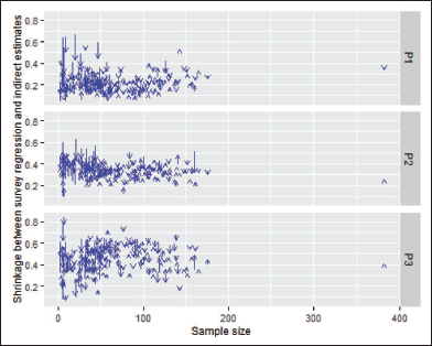
As expected, and shown in Figure 3, areas with smaller sample size have more significant shrinkage towards the means than areas with larger sample sizes. When sample sizes are greater than 100, model predictions and the survey regression estimates become much more similar. We note that there is one county that has sample size around 160 with larger shrinkage in proportions at Level 2 and proportion at or above Level 3.
Literacy Proportion—Shrinkage Plots of Point Estimates, by Sample Size.
In the interval coverage plots of Figure 4, the credible intervals for areas with large sample sizes mainly cover the survey regression estimates. However, when the sample sizes are small (<50), as expected, some credible intervals do not cover the survey regression estimates because the survey regression estimates are less reliable and contribute less to the model-based estimates.
Literacy Proportion—Indication of Coverage by Credible Interval.
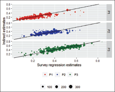
The scatterplot in Figure 5 shows the majority of survey regression estimates and indirect estimates around the 45∘ line. That is, the model predictions are generally close to the survey regression estimates. Counties with larger sample sizes, indicated by larger bubbles, have closer estimates than counties with smaller sizes. As expected, some of the small counties are farther away from the 45∘ lines because of their large sampling errors. Likely due to P1 and P3 being in the model fit and estimation, the proportion at or below Level 1 (P1) and proportion Level 3 and above (P3) have closer estimates than proportion at Level 2 (P2).
Literacy Proportion—Comparison Between Survey Regression Estimates and Indirect Estimates.
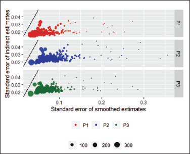
The plot in Figure 6 shows that for areas with small sample sizes, the posterior standard deviations from the SAE model are smaller than the smoothed standard errors of the survey regression estimates and the posterior standard deviations from the SAE model. For these plots, because the standard errors of proportions depend on the sizes of the estimated proportions, the model proportion could be different from the survey regression proportion, and therefore the variance will in theory be different.
Literacy Proportion—Comparison Between Model Standard Errors and Smoothed Standard Errors.
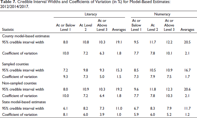
The precision of the model-based estimates depends heavily on the ability of the covariates in the model to predict the outcomes. The model-based estimates produced for counties not in the sample, therefore, rely almost entirely on the model predictions, with some contributions from the division and/ or state random effects. The model-based estimates for counties that were included in the sample (and for which direct estimation is possible) also relied heavily on the model predictions because their direct estimates were based on small samples and are generally imprecise. Table 7 summarizes the distributions of the widths (the difference between the upper bound and the lower bound) of the credible intervals as well as the coefficients of variation (CVs) for the 3,142 counties and 51 states in the United States, for literacy proportion at or below Level 1. Overall, the state predictions are more precise than the county predictions, and to a less extent, the counties with the sample are more precise than counties without the PIAAC sample. For example, for the proportion at or below Level 1 in literacy, the median credible interval width for county predictions is 8.0 percentage points, while the median is 6.1 percentage points for state predictions. Also, the median credible interval width is 7.2 percentage points for counties with the PIAAC sample and 8.0 percentage points for counties without the PIAAC sample. The CVs for the county-level model predictions are of the order of 10%. Estimates with CVs of this magnitude are considered precise.
Credible Interval Widths and Coefficients of Variation (in %) for Model-Based Estimates: 2012/2014/2017
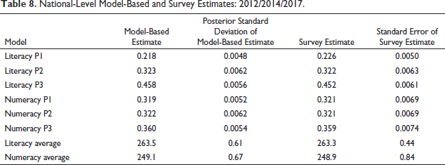
A comparison is shown in Table 8 between the national-level model predictions and the direct estimates for proportions and averages for literacy and numeracy. Because the two sets of estimates are not significantly different, it shows that benchmarking to national direct estimates was not necessary and that the use of a threefold model helps to reduce the need for benchmarking.
National-Level Model-Based and Survey Estimates: 2012/2014/2017
Limitations and Summary
Covariates that have associated sampling or non-sampling error (e.g., possible systematic bias due to inaccurate measurements) cause the measurement error to occur in SAE models. The covariates may have inaccurate measurements with a possible systematic bias. The SAE model results rely on the precision of the covariates and the correlation between the outcome of interest and the covariates. SAE models in the literature with covariates at low levels of geography, such as census tracts, or cross-tabulations of county-level variables from the ACS, have the substantial sampling error or measurement error associated with them. An approach has been provided to allow the propagation of the measurement error into the small area estimates. 28 However, because the approach may not be able to extend to this many variables, we have not accounted for this source of measurement error. When the covariate sampling error exists (measurement error) and is not accounted for, the model is mis specified and will misstate the prediction MSE. 29 An exception is when counties with the sampling error for the covariates equal the average sampling error across the counties. It is interesting to note that the resulting prediction error is generally an overestimate when the county’s sampling error is below average, and more severely underestimates when above average. Small counties likely have less precise ACS data; therefore, cautionary notes are provided on the state- and county model-based estimates website that alert users that the covariates used in the model or predictions for counties with population less than 1,500 (2% of counties) may have higher associated uncertainty.
One feature of the PIAAC SAE process was that models account for informative sampling and informative nonresponse; otherwise, the process would have resulted in biased estimates. The set of counties were selected by way of probability proportionate-to-size sampling; therefore, the sample design is informative. To address the issue of informative sampling, we included the probability of selection of PSUs in the covariate selection process. Because it was not an important factor, it was decided to exclude it from the final SAE model. Also, to help address informative nonresponse, weighting adjustments can be effective if the weighting variables are associated with the proficiency scores. Literacy-related nonresponse (about five percent) was also addressed through imputation of low scores prior to creating the direct estimates.
Second, another feature was that the models accounted for all important sources of variability so that the reported estimated error reflects the true level of precision. For PIAAC, these sources of error include the following: (a) the sampling error, (b) model error (c) the prediction error and (d) the imputation error.
The sampling error results from probability sampling and from the fact that different results would occur for repeated samples. Likewise, the imputation error results from the generation of PVs and that different results would occur for replications of the imputation process. The uncertainty due to sampling and imputation has been accounted for in the SAE process and captured in the HB model. The model error results from the estimation of model parameters, such as area-level random effects. This type of error accounts for different results occurring for different runs of the modelling process due to its random mechanism in fitting the models. The HB method accounted for the noise contributions attributed to estimating model parameters (beta coefficients and random effects variance-covariance parameters). The prediction error results from making estimates from the final model for areas (including those without PIAAC sample cases) and are accounted for in the resulting credible intervals.
Although the modelling process allows various sources of error to propagate into the results, the following model features have been implemented to reduce the amount of error. The SRE approach reduces the amount of error associated with the survey estimates. In addition, the thorough covariate selection process results in strong models, which included the bivariate model for the proportions. The model also takes advantage of the covariance between domains by using the same covariates for each domain.
Finally, the three levels of random effects - county, state and census division (threefold model) ensure that estimates are not fully synthetic. That is, states that do not have the PIAAC sample will have some contribution from the PIAAC sample because all census divisions have the PIAAC sample. Furthermore, because the same random effect is applied to counties within states, and states within division, the associations of counties within states and states within divisions will have some impact.
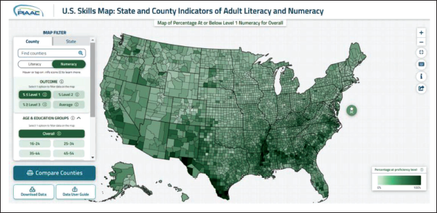
The resulting estimates are accessible through the PIAAC Skills Map for State and County Indicators of Literacy and Numeracy. 2 The Skills Map provides interested users the ability to analyse and explore the model-based estimates through heat maps and allows for statistical comparisons between counties, between counties and their state, between states, and between states and the nation. Figure 7 shows a heat map for the county model-based estimates for the proportion at or below Level 1 numeracy.
County-Level Heat Map of Model-Based Proportions at or Below Level-I Literacy.
Footnotes
Acknowledgements
The authors are grateful for the guidance provided by J. N. K. Rao, who was a consultant on the project during both the NAAL and the PIAAC SAE processes. Also, the contributions of Weijia Ren to the evaluation and graphs were much appreciated. In addition, Partha Lahiri, William Bell and Danny Pfeffermann provided some important feedback in the early stages of model development as members of the international SAE expert panel convened by NCES. The authors greatly appreciated the reviewer comments which improved the manuscript.
Declaration of Conflicting Interests
The authors declared no potential conflicts of interest with respect to the research, authorship and/or publication of this article.
Funding
The authors disclosed receipt of the following financial support for the research, authorship, and/or publication of this article: The research and development of the SAE models was conducted under contract to the National Center for Education Statistics.