
Abstract
ISTAT has recently released an updated version of short-term statistics on hours worked in Italy, which are used in labor input estimates by the Quarterly National Accounts (QNA). The coverage of these statistics has been expanded from larger-than-ten workers firms to include the entire universe of Italian private firms. To include the updated indicator within estimates by QNA, the series must be reconstructed back to 1995 first quarter (1995q1) due to methodological requirements of QNA. In this paper, we first reconstruct the updated indicator using the Kalman filter and smoother algorithms applied to a state-space representation of a multivariate structural model (SUTSE). Next, we comparatively assess the performance of the new indicator against the non-updated one. This assessment is based on estimates of quarterly per-employee hours worked using temporal disaggregation methods for seven economic sections spanning the non-agricultural private business economy over the period 1995q1 to 2020q4. Compared to the previous indicator, the reconstructed indicator (i) implies improvements in temporal disaggregation model fitting in the majority of economic sections considered; (ii) returns smaller forecast errors in the 64.3% of the estimations, based on MAE; (iii) ensures a higher correlation between the estimated quarterly series to the indicator in the 71.4% of the estimates.
1. Introduction
Since mid-eighties, the Italian National Institute of Statistics (ISTAT) has been systematically disseminating Quarterly National Accounts (QNA) data. ISTAT employs an indirect estimation approach for QNA, primarily based on temporal disaggregation (TD) techniques. These techniques employ high-frequency reference indicators and are applied to the corresponding Annual National Accounts (ANA) totals. Historically, estimation approaches have relied on static regression methods such as Chow and Lin (1971), Denton (1971), and Fernàndez (1981). Notably, in 2019, the set of models was expanded to include dynamic regression methods based on autoregressive distributed lag (ADL) models, in line with the approach suggested by Proietti (2006).
Short-term reference indicators used in the production of QNA mainly originate from monthly or quarterly statistics produced by ISTAT surveys (e.g., Industrial Production Index, Labour Force, Services Turnover, etc.). The present analysis focuses on the quarterly estimates of per-employee hours worked by QNA. These estimates are obtained through TD methods using “per-employee hours worked” statistics derived from the ISTAT survey on job vacancies and hours worked (VELA survey) as reference indicator. The estimates of per-employee hours worked are then multiplied by the estimates of employee jobs to obtain employees total hours worked by QNA. Finally, these figures are benchmarked with the corresponding ANA totals to ensure consistency between quarterly and annual data.
Until June 2019, the VELA survey exclusively provided quarterly index statistics for non-agricultural private firms with at least ten workers. These statistics, expressed in levels, serve as the current reference indicator for estimating hours worked within QNA. However, in compliance with regulatory requirements from the European Commission (EC Reg. N. 1165/98 and subsequent modifications), the VELA survey expanded its coverage as of June 2019 to include all private firms with employees. The updated index statistics, available from 2015q1 onwards, have been released in a seasonally non-adjusted form.
The exclusion of micro firms (those with fewer than ten workers) from the short-term indicator used for the estimation of hours worked by QNA can lead to three main inconsistencies. First, there may be inconsistency with respect to ANA totals of hours worked referring to the entire population of resident firms as established by the European system of national and regional accounts ESA 2010 (EU 2013). Second, there could be inconsistency with the estimates of other labor input aggregates (e.g., self-employed hours worked, employment, full-time equivalent) and labor cost by QNA, both relying on short-term indicators (e.g., Labour Force survey indicators or administrative data-based surveys) referring to the whole population of firms. Third, there might be inconsistency with estimates of value added by QNA, with a potential impact on the accuracy of labor productivity measure.
The use of the updated indicator from the VELA survey in principle has the potential to address the drawbacks associated with the use of the indicators excluding micro firms. Moreover, the improved alignment between the coverage of the updated indicator and the definition of National Accounts (NA) aggregates should enhance the performance of TD models. This could lead to a better fit between the quarterly estimates and the annual aggregates, reducing the amount of revisions and improving the quality of the extrapolated observations.
Quarterly series in ISTAT are compiled and estimated at each release over the whole period starting from 1995q1 (ISTAT 2023). Hence, the introduction of the updated indicator from the VELA survey, including data for all private firms with employees from 2015q1 onwards, calls for data reconstruction back to 1995q1 within the estimation of QNA by TD models.
The present contribution aims to accomplish two main objectives: first, reconstructing the updated indicator of per-employee hours worked (expressed in levels) from 2015q1 back to 1995q1; and second, assessing the performance of the reconstructed extended indicator in the estimates of per-employee hours worked by QNA, compared to the performance of the indicator currently in use.
Concerning the reconstruction, we employ a model-based approach, specifically opting for the class of structural time series models (Harvey 1990). In this case, we utilize a bivariate structural model in which both the updated and the non-updated indicators are endogenous. The non-updated indicator, available throughout the entire time span considered (i.e., from 1995q1 to 2021q4), serves as a proxy for the missing data in the extended indicator from 2014q4 back to 1995q1.
The advantage of this approach lies in the statistical treatment of the model that can be carried out by the Kalman filter and smoother algorithms. The latter allows for a diffuse representation of starting conditions within the state-space representation (Koopman 1997) and facilitates the reconstruction of missing observations of the shorter indicator as a by-product of the algorithms. Additionally, this approach enables the overcoming of certain restrictive hypotheses and limitations that are inherent in relatively more naïve back-calculation approaches, such as proportional methods or regression approaches (Caporin and Sartore 2006).
To evaluate the performance of the extended indicator, the empirical strategy involves the application of TD methods to the annual per-employee hours worked by ANA, alternatively using the non-updated and the updated reconstructed indicator as reference indicator. The estimations span is from 1995q1 to 2020q4, covering the non-agricultural business economy (i.e., economic sections from BCDE-to-MN according to NACE rev.2). Indeed, although hours worked estimates within QNA are conducted at the NACE rev. 2 section detail (from section A to T), the use of indicators from the VELA survey is limited to the estimates of sections from B to N. This limitation is attributed to both the coverage of the VELA survey, which is confined to private firms (sections from B to S), and the fact that non-business services (sections from O to S) mainly consist of non-market economy activities.
Multiple TD model specifications, such as the Chow-Lin (1971) and Fernàndez (1981) models, have been employed, due to their frequent application in QNA estimates. The chosen time interval aligns with the current availability of ANA final totals derived from structural statistics, with only provisional ANA figures accessible for the subsequent period (i.e., 2021 onwards) at the time of writing. Performance evaluation of the two indicators relies on both diagnostic statistics of the estimated models and computed statistics measuring the forecasting errors of the fitted model, along with the quality of disaggregated observations. Diagnostic statistics encompass goodness-of-fit measures, such as computed information criteria and coefficients of determination. The forecasting performance of the models is assessed using standard statistics gauging the size of out-of-sample forecast errors. Finally, the quality of temporal disaggregation models is evaluated by examining both the correlations and coherence of signs between the quarterly and annual dynamics of the indicator series and the estimated output series by TD.
The results indicate that the reconstructed indicator enhances the fitting of the temporal disaggregation model in the majority of the examined economic sections when compared to the non-updated one. Additionally, the use of the reconstructed indicator yields smaller forecast errors than those obtained using the non-updated indicator in most estimations, according to Mean Absolute Error (MAE). Moreover, it ensures a higher correlation between the estimated quarterly series and the indicator in 71.4% of the estimates. Both indicators are equally satisfactory in terms of coherence with the dynamics of the disaggregated series, irrespective of the model used.
The remainder of the paper is structured as follows: Section 2 delves into more details on the method employed for data backwards reconstruction and presents the results of the structural model estimations. Section 3 provides descriptive evidence on the indicators and ANA data, along with a detailed comparison of the performance of the restricted and extended indicators in the temporal disaggregation exercise. Finally, Section 4 offers conclusive remarks.
2. Model-Based Backwards Reconstruction of the Indicator
Backwards reconstruction, also known as back-calculation, involves estimating unavailable past values of economic variables at the desired frequency using all available relevant information. However, several factors should be considered when choosing a methodological strategy for back-calculating a time series from existing approaches (e.g., retropolation, interpolation, regression methods). These factors include the availability of a related series, its availability at the desired frequency, the microeconomic versus macroeconomic dimension of the data, and the presence of cross-sectional or time constraints to be respected (United Nations 2018).
The present analysis employs a model-based approach to backwards reconstruction, specifically relying on the class of structural models (Harvey 1990). In particular, we consider a bivariate version of a basic structural model. In this model, both the non-updated indicator (referred to as “10+” hereafter, covering firms larger than ten workers) and the updated indicator (referred to as “TOT” hereafter, covering the totality of private companies) serve as dependent variables. This strategy offers several advantages compared to alternative approaches that utilize related information (i.e., time series) for the series to be reconstructed. First, unlike the Ordinary Least Squares (OLS) framework, which involves regressing the “short” series against the “long” series to estimate a proportional beta coefficient, a structural model-based approach is not constrained by the exogeneity hypothesis of the “x” terms, which can be unrealistic in this context. Second, in contrast to plain retropolation methods, this approach does not assume that the reconstructed and the reference series are linked by a constant proportional relationship over the entire period.
Third, among methods not involving the use of related information, a structural model-based approach outperforms univariate Auto Regressive Integrated Moving Average (ARIMA) models. Indeed, univariate ARIMA models, involving reversing the series, fitting the model, and producing forecasts to predict the past, have a limited backwards forecast capacity (Caporin and Sartore 2006).
The statistical treatment, can be effectively managed by the Kalman filter (KF hereinafter) (Kalman 1960) applied to the model in the state-space form (SSF) (Durbin and Koopman 2012; Koopman et al. 1999) where the reconstructed observations result as a by-product of the smoothing algorithm.
The effectiveness of the KF in the context of missing observations and data reconstruction is well-known (Gómez and Maravall 1994; Harvey 1990; Harvey et al. 1998), finding application in various model classes such as dynamic factor models (Poncela et al. 2021) and structural models (Koopman et al. 2007; Moauro 2001; Moauro and Savio 2005).
Among the advantages of a SSF and the use of KF it is worth mentioning: (i) the availability of a rich set of diagnostic statistics on the quality of the estimated model; (ii) the backwards reconstruction of the time-series as a by-product of the KF smoothing algorithm where the whole available information set over the time interval is efficiently used; (iii) the opportunity for a formal treatment of the initial conditions (initialization of the KF algorithm) that can be optimally estimated (Koopman 1997).
2.1. Structural Models in This Application
According to the structural time series models framework (Harvey 1990), a time series
with

where mt has to be initialized to a starting value m0.
In the absence of the slope component (
Alternatively, if the slope is present but has a deterministic form (
Finally, if a deterministic level (

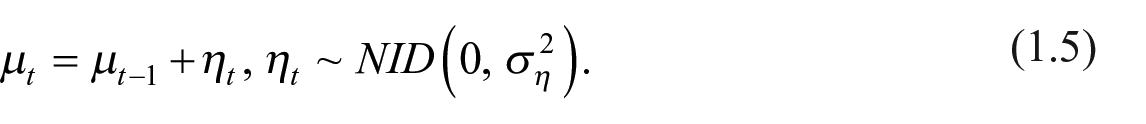
The multivariate generalization of the univariate structural model is known as Seemingly Unrelated Time Series (SUTSE) models (Harvey 1990). In our application, we consider a bivariate SUTSE model with LLT specification plus a seasonal component (

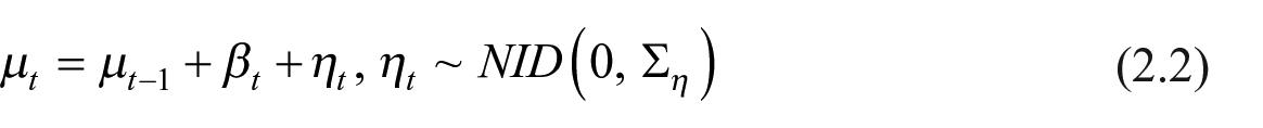
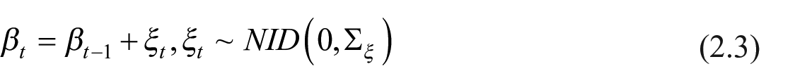
where
The seasonal component (
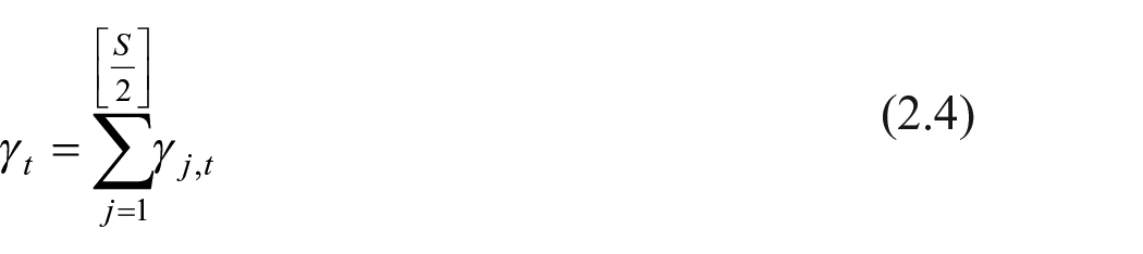
where each
where:
For each component i, the bivariate (2 × 1) vector of white-noise errors are characterized by zero mean and (2 × 2) unknown variance-covariance matrices (
For
SUTSE models allow for common factor restrictions (Koopman et al. 2007) which imply the covariance matrices of the relevant disturbances of one (or multiple) component(s) are less than full rank. In the case of a general LLT model, the series may share a common pattern over either the level, slope, seasonal, and/or the irregular component. Common trends arise in case of either common levels and/or common slopes. When restricted version of the LLT model are considered, common trend may arise in turn on levels (LL, RWD) or the slope (IRW) stochastic component. In general, the presence of a common factor in the multivariate LLT model with N series is that the rank of matrices
In general, the cointegration of two series ensures that a common stochastic trend drives their long-run behavior. This proves favorable within the reconstruction framework, when a “long” series is available as a reference indicator to infer the “short” one. Indeed, cointegration implies that the reconstructed series would, at least, not diverge from the observed series—a convenient aspect in official statistics where transparency is appreciated by the users. In the case of common trends, the observed and reconstructed series would span parallel paths, while cointegrated seasonality would induce aligned seasonal patterns between the two series.
The statistical treatment of structural models in this application is based on the state-space representation (SSF) of the model and the use of the KF (Harvey et al. 1998; Koopman et al. 2007). The SSF is characterized by two equations: the first describes the time series structure (measure equation), the second equation describes the transition of the structural latent components from one state to the following one (transition or state equation). The application of the KF to the SSF allows to compute an optimal estimator of the state variables vector at time t for t = 1,. . .,T, given the information available in t. By contrast, the associated smoothing algorithm allows an optimal estimation of the state vector, given the whole information set, that is, until time T. In the present context, given
2.2. Reconstructing Per-Employee Hours Worked Series
The object of the reconstruction is the series on per-employee hours worked in levels, which is disseminated on a quarterly basis by the VELA survey in index form. The non-updated indicator (10+) refers to companies with at least ten workers and is available from 1995q1 onwards, whereas the updated version (TOT) covers all firms with employees and is available from 2015q1 onwards. The scope of the reconstruction exercise is limited to the non-agricultural business economy (from B to N according to NACE rev.2) aligning with the breakdown of economic activities adopted for the estimates of labor input by QNA (see Appendix, Table A2). In Figure 1, both indicators, in index form, are plotted for the selected sections over their respective available span. The dynamics of the two series appear highly correlated in the overlapping period (2015q1–2022q4) for the majority of sections.
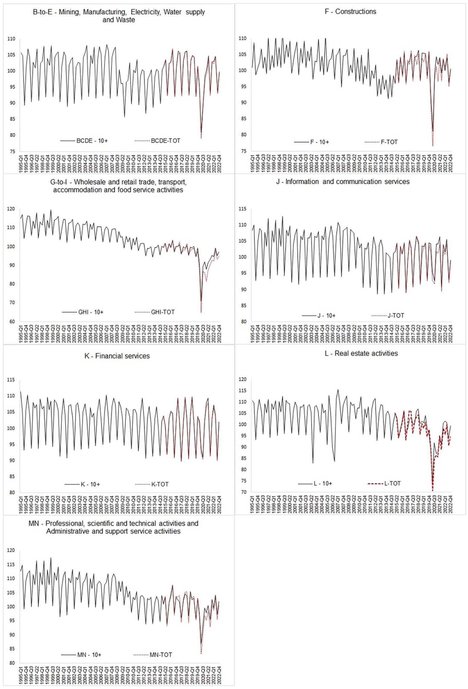
Per-employee hours worked index according to TOT and 10+ indicator, respectively. 1995q1 to 2022q4 (2015q1–q4 = 100). Non-seasonally adjusted data.
The structural model described by Equation (2.1) to (2.4) is considered, where the bivariate dependent
The KF is applied to the SSF representation of Equation (2.1) to (2.4), providing the estimates of the related log-likelihood and the unknown parameters. The smoothing algorithm efficiently estimates the state vector and the error vector using both past and future observations. As a by-product of the latter, the estimation of the observations of the TOT indicator for the 1995q1 to 2014q4 time span (eighty quarterly observations) is obtained.
Using the programming language Ox, model estimation is performed by the STAMP package (Koopman et al. 2007) that uses the Broyden-Fletcher-Goldfarb-Shanno (BFGS) approximation method for the maximization process. Table 1 presents selected estimated parameters for the seven estimated models, namely: the estimated maximum of the sample log-likelihood (
Estimated Parameters From the BiVariate SUTSE Model Fitted to Data From 2015q1 to 2021q4.
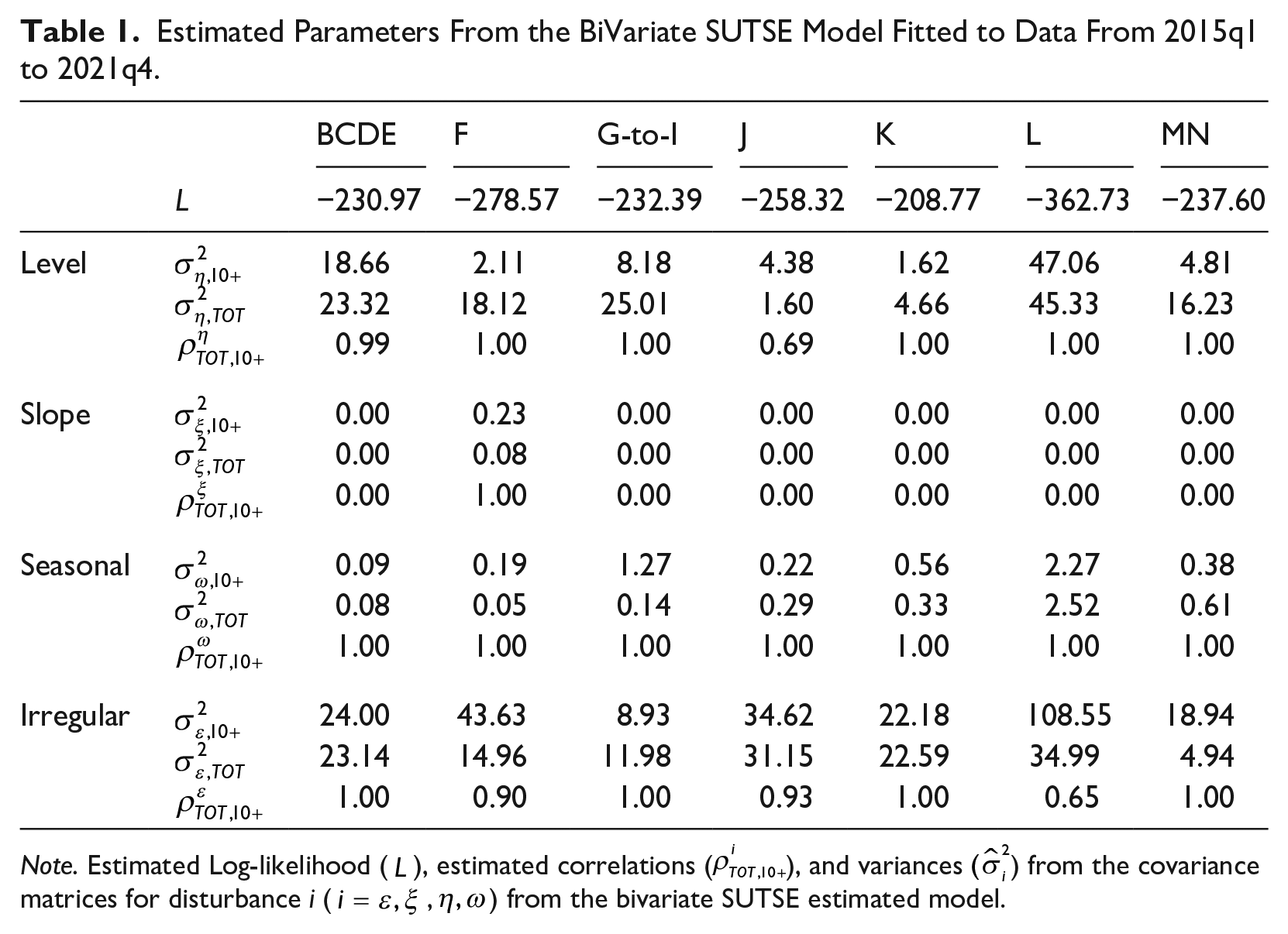
Note. Estimated Log-likelihood (
A brief inspection of Table 1 reveals that overall the level component disturbances are highly correlated—as revealed by
Table 2 presents diagnostics derived from the expected residuals of the estimated models, along with the coefficient of determination. The diagnostics indicate that the null hypotheses for both normality and homoscedasticity of the residuals cannot be rejected for the entire set the estimated models. Additionally, there is no evidence of first-order autocorrelation in the residuals across all estimates as indicated by both the N-statistics and Durbin-Watson (DW) statistics (Durbin and Watson 1950, 1951) for both the 10+ and TOT series. According to the Ljung-Box Q-statistics (Ljung and Box 1978), the null hypothesis of the absence of autocorrelations in the first eight lags is never significant for the TOT series. However, in the case of the 10+ series, the null hypothesis cannot be rejected in more than one instance (F, GHI, K, L, MN). Overall, the model fitting is deemed satisfactory, as indicated by R2 values.
Summary Statistics From the BiVariate SUTSE Estimated Model. a
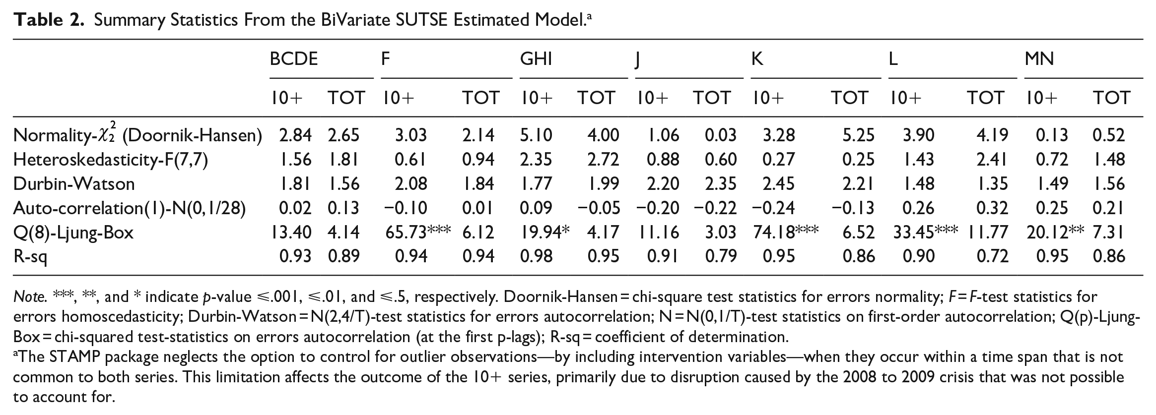
Note. ***, **, and * indicate p-value ⩽.001, ⩽.01, and ⩽.5, respectively. Doornik-Hansen = chi-square test statistics for errors normality; F = F-test statistics for errors homoscedasticity; Durbin-Watson = N(2,4/T)-test statistics for errors autocorrelation; N = N(0,1/T)-test statistics on first-order autocorrelation; Q(p)-Ljung-Box = chi-squared test-statistics on errors autocorrelation (at the first p-lags); R-sq = coefficient of determination.
The STAMP package neglects the option to control for outlier observations—by including intervention variables—when they occur within a time span that is not common to both series. This limitation affects the outcome of the 10+ series, primarily due to disruption caused by the 2008 to 2009 crisis that was not possible to account for.
The reconstruction of the time series based on KF algorithms allows for the assessment of the precision of the estimates based on the estimated standard errors. This feature stands as an advantage over alternative reconstruction methods—such as retropolation and proportional methods. In Figure A1 in the Appendix, the reconstructed series derived from the structural models is depicted, along with 95% confidence interval bands. As anticipated, the precision of the estimates noticeably diminishes when moving from 2014q4 to the beginning of the time span, as indicated by wider confidence bands.
As a further assessment of the quality of the reconstructed series by the structural model, we calculated the correlation between the annual totals by ANA and the annualized indicators reconstructed using two alternative approaches. Namely, (i) the proportional method, which entails retrieving the beta estimated coefficient from the regression of the TOT indicator over 10+ indicator over the common interval and, as a second step, multiplying the beta coefficient by the observations of the 10+ series over the span of 1995q1 to 2014q4 to obtain the missing observations; (ii) a retropolation approach, which applies year-on-year back-growth rates from the 10+ quarterly series to the TOT quarterly series over the blank span from 1995q1 to 2014q4. Table A2 shows that the quarterly series obtained by structural models ensures a higher, or at least comparable, correlation at the annual frequency with ANA totals compared to the alternative methods considered. It is noteworthy that the model-based approach proves preferable in this context, despite the relatively greater data demands of the Kalman Filter (KF) estimation in structural models compared to, for example, linear models (proportional methods), where a smaller amount of parameters has to be estimated. Importantly, the higher the correlation between the high-frequency indicator and the low-frequency series, which serves as the longitudinal benchmark for the high-frequency estimates, the better the TD model should fit and the higher its out-of-sample forecast capacity is expected.
3. Temporal Disaggregation of Per-Employee Hours Worked
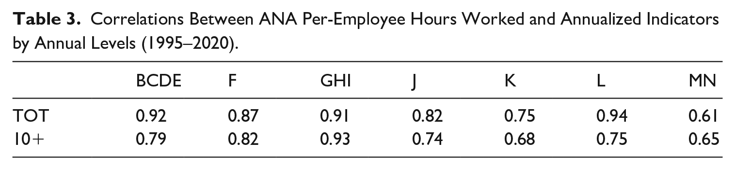
After obtaining the reconstruction of the TOT indicator (see Appendix, Figure A2), we assess its performance in a temporal disaggregation exercise. This exercise allows us to determine if and to what extent the transition to the new indicator would enhance the quality of quarterly estimates of per-employee hours worked by QNA, as compared to the current estimates based on the 10+ indicator. Given its inherent higher correlation with ANA totals, the primary assumption of this application is that the quarterly TOT indicator should improve the temporal disaggregation estimates compared to the 10+ series, in terms of both goodness of fit and out-of-sample forecast performance. The latter is a by-product of the statistical approach adopted to derive quarterly estimates of NA aggregates at ISTAT, which relies on the SSF representation of reference models (e.g., Chow-Lin, Fernández, ADL), and the associated use of the Kalman filter (Bisio and Moauro 2018). A preliminary examination of the relationship between ANA per-capita hours worked and the annual averages of TOT and 10+ indicators, spanning from 1995 to 2020, reveals a consistently high correlation for both indicators with the annual totals. Notably, the TOT indicator exhibits higher correlation values across the majority of the sections of interest, as presented in Table 3. Indeed, a visual inspection confirms very similar paths in the annual growth rates between the two indicators throughout the entire period (Figure 2), with the dynamics of the 10+ series during the 2020 crises—particularly in F, GHI, and K sections—closely mirroring that of ANA totals more closely than the TOT indicator.
Correlations Between ANA Per-Employee Hours Worked and Annualized Indicators by Annual Levels (1995–2020).
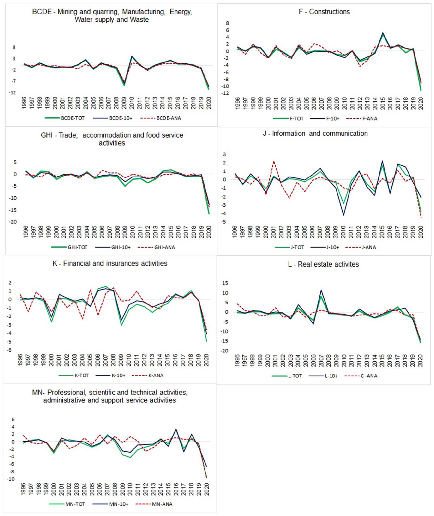
Per-employee hours worked by annualized indicators (10+ and TOT) and Annual National Accounts, 1995 to 2020. Annual growth rates.
Temporal disaggregations are carried out over the 1995q1 to 2020q4 interval, using final estimates of ANA that are not subject to structural revisions. Indeed, the restriction of the time span of the application up to 2020 is motivated by the fact that it is the last year for which ANA figures will not undergo future revisions, at the time of writing, consistently to the revisions policy of ANA in ISTAT. The analysis covers the non-agricultural business economy (from BCDE to MN section, according to NACE rev.2), consistent with the breakdown of per-employee hours worked estimates by QNA (Table A2). ANA totals of per-capita hours worked are regressed over, alternatively, the TOT indicator and the 10+, in a non-seasonally adjusted form. The temporal disaggregation models considered are, in turn, Chow and Lin (1971) and Fernàndez (1981) with and without the intercept term, respectively. In other words, four temporal disaggregation model specifications are run for each of the seven economic sections considered, resulting in a set of twenty-eight outcomes by distinct estimated models.
Table 4 displays the main outputs and diagnostic statistics derived by the “best” model specification obtained among the set of four TD model specifications, for each section where the two indicators are used alternatively. For each section, we select the specification with the best performance in terms of information criteria (AIC/BIC) and Log-likelihood out of the four estimated specifications. In this respect, it is worth noting that the same model is selected for each given sector, regardless of the reference indicator used.
Regression Diagnostic Statistics on Quarterly Disaggregation of Per-Employee Hours Worked, Non-Seasonally Adjusted Data, 1995q1 to 2020q4.
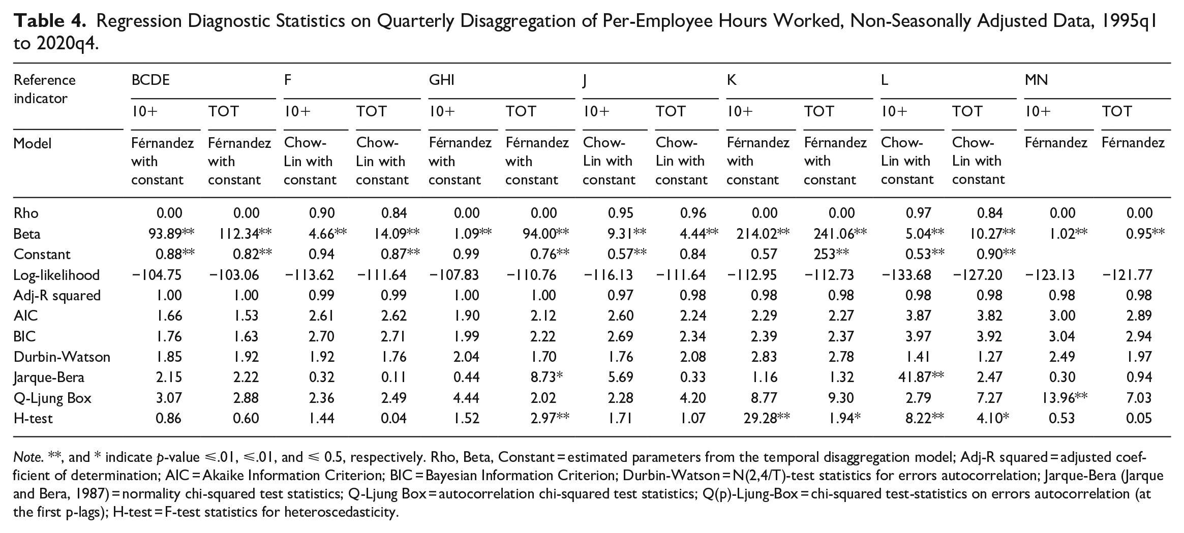
Note. **, and * indicate p-value ⩽.01, ⩽.01, and ⩽ 0.5, respectively. Rho, Beta, Constant = estimated parameters from the temporal disaggregation model; Adj-R squared = adjusted coefficient of determination; AIC = Akaike Information Criterion; BIC = Bayesian Information Criterion; Durbin-Watson = N(2,4/T)-test statistics for errors autocorrelation; Jarque-Bera (Jarque and Bera, 1987) = normality chi-squared test statistics; Q-Ljung Box = autocorrelation chi-squared test statistics; Q(p)-Ljung-Box = chi-squared test-statistics on errors autocorrelation (at the first p-lags); H-test = F-test statistics for heteroscedasticity.
Overall, the estimates exhibit satisfactory results, in terms of both goodness of fit and linearity and independence of the residuals. These outcomes are qualitatively similar when comparing the use of the two alternative indicators. However, some concerns arise in sections K (financial services) and L (real estates) regarding both non-normality of errors and errors autocorrelation (at the 8-lag), regardless of the indicator used. The absence of autocorrelated errors at the first lag is overall confirmed by Durbin-Watson statistics, independently of the indicator used. Nevertheless, the use of TOT implies slightly higher log-likelihood values and lower values of the information criteria (AIC, BIC) in the majority of cases, except for two relevant sectors (GHI and F). Lastly, the hypothesis of errors homoscedasticity is accepted at the 95% of confidence in the majority of sections (namely, BCDE, F, J, and MN), while it is rejected in a couple of cases (K and L) irrespectively of the indicator used, and for GHI sector when using the TOT indicator.
To compare the out-of-sample forecast performances of the two indicators we compute both the mean absolute error (MAE) and the root mean squared error (RMSE) referred to the difference between the growth rates of ANA totals and the annual growth rates resulting from the sum of the four extrapolated quarters over the annual totals of the previous year. Both the statistics are computed on the last eight annual observations of the series (2013–2020). In essence, both metrics measure the out-of-sample forecasting performance of the indicators in terms of low-frequency (i.e., annual) estimates—with large errors weighted relatively higher by RMSE. Lower values in these metrics imply smaller revisions between the annual totals derived by quarterly figures estimated by the TD model and ANA.
Table 5 reports both MAE and RMSE computed for each temporal disaggregation model specification that has been tested, employing the two indicators under evaluation alternatively. According to MAE, TOT indicator outperforms 10+ indicator in eighteen cases over twenty-eight estimates, while according to RMSE, TOT indicator outperforms 10+ indicator in twenty cases over twenty-eight estimates. Overall, we observe that the use of the TOT indicator results in a smaller forecast error at the annual frequency in the majority of cases when estimating QNA over the business economy sections. Namely, the improvement occurs in the 64.3% and 71.4% of cases, according respectively to MAE and RMSE.
MAE and RMSE of Annual Growth Rates by ANA and Extrapolated Quarters by Temporal Disaggregation Estimates, 1995q1 to 2020q4.
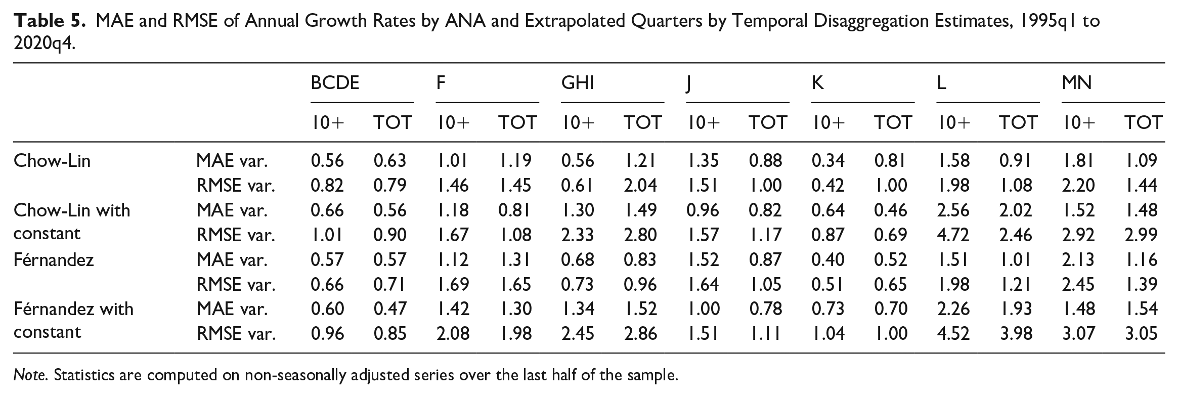
Note. Statistics are computed on non-seasonally adjusted series over the last half of the sample.
Moreover, to assess the quality of the disaggregated series in terms of association to the reference indicator used, we both (i) compute the correlation and (ii) test the coherence of signs between the quarterly disaggregated series and the indicator used, considering both quarter-on-quarter (q-o-q) and year-on-year (y-o-y) growth rates. In particular, the coherence of signs is assessed by a binomial test where the probability of success (i.e., consistency of signs in q-o-q/y-o-y changes between the indicator and the output series in each quarter) under the null hypothesis is p = .5. Differently than MAE/RMSE, both these metrics provide a measure of the quality of TD models at the high (quarterly) frequency.
Table 6 reports the correlations for each of the estimated model, computed over the last half span of the series that is, 2007q4 to 2020q4. Overall, higher correlations, whether based on “q-o-q” or “y-o-y” growth rates, between the disaggregated series and the reference indicator are identified in twenty out of twenty-eight estimated models when the TOT indicator is used (71.4%), as compared to the 10+ indicator. It is worth noting that, irrespective of the model specification, TOT indicator outperforms the alternative one in sections F, J, L, and MN. Conversely, the 10+ indicator ensures higher quality in section GHI, regardless of the model specified. By contrast, a mixed evidence emerges for BCDE and K sections where the superiority of one indicator over the other depends on the specified model.
Correlations Between Q-o-q Growth Rates and Y-o-Y Growth Rates of Indicators and Disaggregated Series by Temporal Disaggregation Estimates Over 1995q1 to 2020q4.
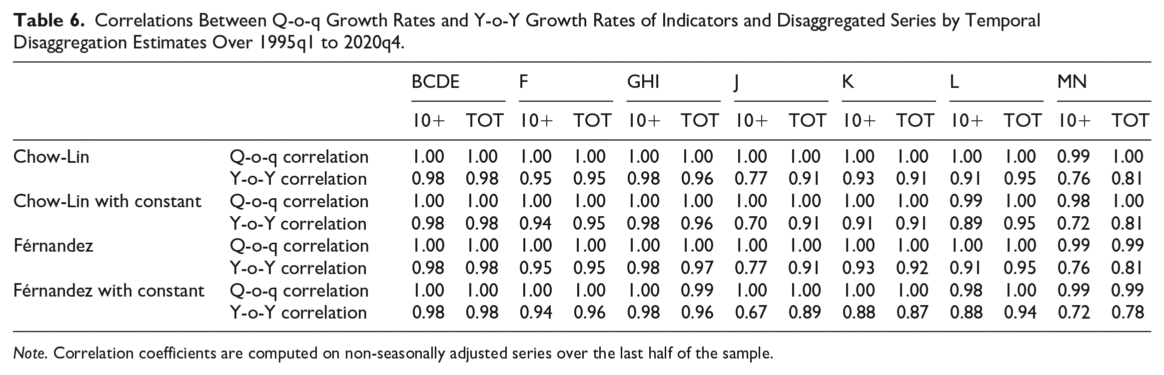
Note. Correlation coefficients are computed on non-seasonally adjusted series over the last half of the sample.
Finally, we investigate the extent to which each indicator, respectively, co-moves with the disaggregated series by checking the coherence of signs, considering both their “q-o-q” and “y-o-y” changes. Table 7 reports p-values from a sign test based on a one-sided binomial distribution at the 95% confidence level. The results highlight that dynamics direction of both TOT and 10+ indicators follows that of the disaggregated series, both on a quarterly and annual basis. Specifically, the null hypothesis of a lower-than 0.5 probability of growth rate signs coherence is rejected with 95% of confidence, regardless of the TD specification used for both indicators, across almost all economic sections. The only exception concerns annual changes for MN section, where the null cannot be rejected for TOT indicator in three cases over four and for 10+ only once.
Sign Test on Q-o-q Growth Rates and Y-o-Y Growth Rates of Indicators and Disaggregated Series by Temporal Disaggregation Estimates Over 1995q1 to 2020q4.
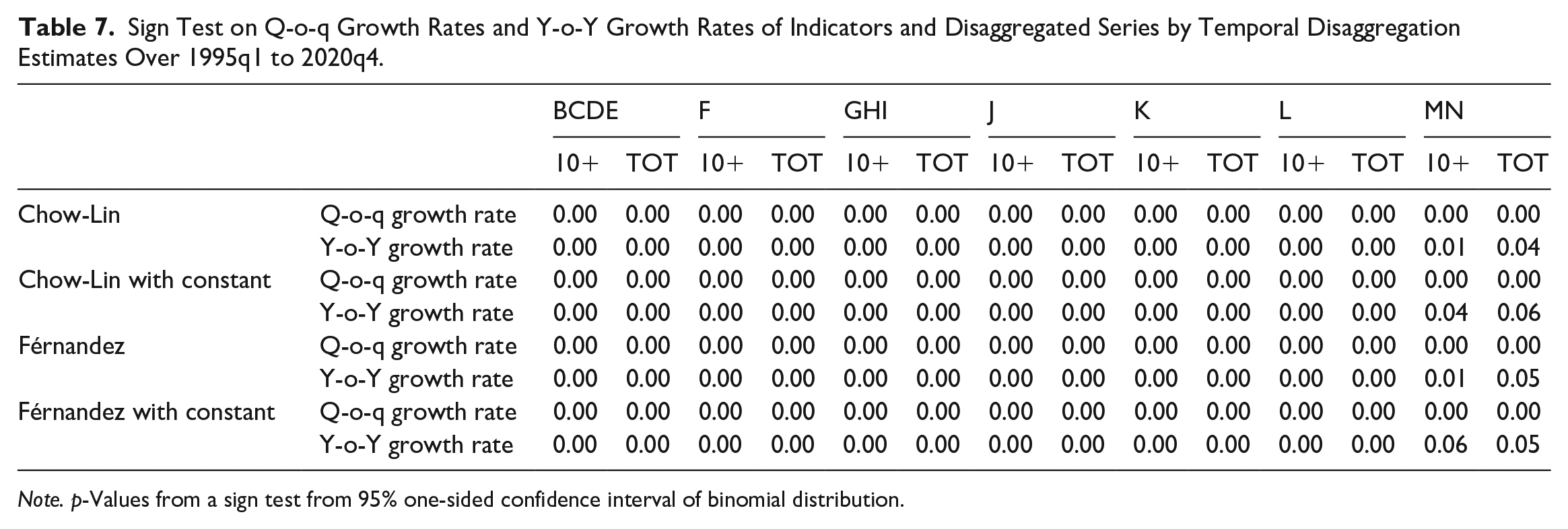
Note. p-Values from a sign test from 95% one-sided confidence interval of binomial distribution.
4. Concluding Remarks
The primary objective of this paper is to pave the way for the integration of a recently released short-term indicator on per-employee hours worked into the estimates of QNA hours worked at ISTAT. Due to its extension to micro-firms, the coverage of the new indicator aligns more consistently with the definitions of labor input by NA, offering advantages in terms of both quality and internal consistency among the estimated aggregates by QNA.
To achieve this objective, the first contribution of this work involves the retrospective reconstruction of the new indicator of per-employee hours worked, to align with the methodological requirements of QNA estimation at ISTAT. Specifically, a model-based approach to backwards reconstruction is proposed, where both the new indicator (covering all firms with employees) and its previous version (covering firms with more than ten workers) are the dependent variables in a bivariate SUTSE model (Harvey 1990). Based on the state-space representation of the model, the Kalman filter and smoothing algorithms enable the recovering of missing observations for the short indicator. Model estimates show that the two indicators share common factors over the trend, the seasonal and the irregular component. In comparison to alternative reconstruction methods, such as retropolation and ordinary least squares (OLS), we observe that the model-based approach yields a reconstructed quarterly series that exhibits a higher correlation with the annual totals reported by ANA at the annual frequency.
The second contribution of the analysis involves the assessment of the advantages derived from the use of the reconstructed extended indicator within the estimates of per-employee hours worked by QNA, in comparison to the use of the previous version of the indicator. The evaluation is based on diagnostics obtained from estimated TD models, employing both the Chow and Lin (1971) and Fernàndez (1981) specifications. Quarterly per-employee hours worked by NA are derived alternately using either the reconstructed or the old indicator. Conducting separate model runs for seven economic sections (NACE rev.2) within the non-agricultural business economy, our findings indicate that the reconstructed TOT indicator leads to slightly higher goodness-of-fit statistics compared to the 10+ version in the majority of the estimated models. Moreover, the predictive power of the models in terms of annual growth rates of the annualized quarterly estimated series is higher when the TOT indicator is used in the majority of cases, based on either MAE (64.3% of cases) and RMSE (71.4% of cases) statistics. Smaller out-of-sample forecasting errors imply smaller revisions in the estimated QNA, when the extrapolated quarters are benchmarked to the annual totals as soon as they become available, representing a valuable outcome for the quality of QNA estimates according to international standards (Eurostat 2018, 2021). Moreover, the reconstructed indicator exhibits higher correlation with the disaggregated series—on both quarterly and annual basis—compared to the 10+ indicator in the majority of the estimated models. This aspect stands as a strong advantage for the quality of the empirical estimates, particularly when extrapolated quarters are released while annual totals are not yet available. In such cases, the short-term indicators serve as the sole information guiding the short-term dynamics of NA estimates and orienting data users.
All in all, based on the presented results, this analysis indicates that the introduction of the updated indicator covering all firms with employees would lead to an improvement in the quality of the estimates of per-employee hours worked by QNA in various respects. However, this evidence represents only an initial step toward the incorporation of such a new source of information into official statistics compilation. The adoption of the new short-term indicator should indeed be complemented by an accurate revisions analysis of the estimates by QNA. Moreover, users and practitioners of NA data should promptly receive explanations about the factors behind data revisions and the economic significance of these revisions.
Footnotes
Appendix A
Comparing Correlation Between ANA Totals and Reconstructed TOT Indicator of Per-Employee Hours Worked (in Levels), According to Alternative Reconstruction Approaches, 1995 to 2014.
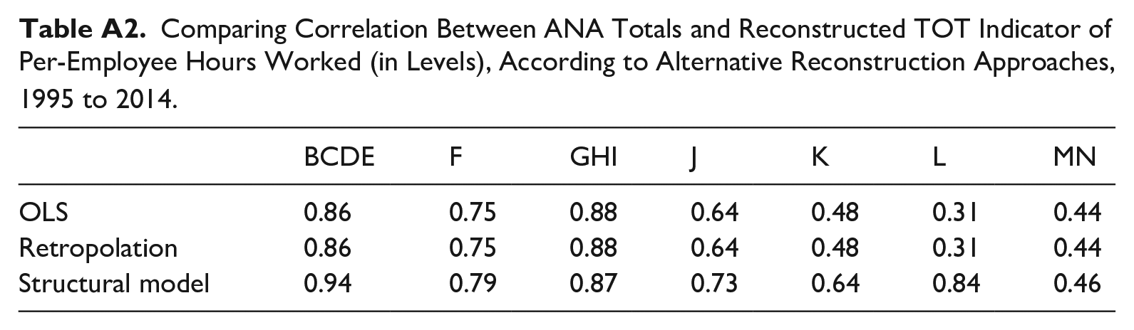
| BCDE | F | GHI | J | K | L | MN | |
|---|---|---|---|---|---|---|---|
| OLS | 0.86 | 0.75 | 0.88 | 0.64 | 0.48 | 0.31 | 0.44 |
| Retropolation | 0.86 | 0.75 | 0.88 | 0.64 | 0.48 | 0.31 | 0.44 |
| Structural model | 0.94 | 0.79 | 0.87 | 0.73 | 0.64 | 0.84 | 0.46 |
Acknowledgements
I am grateful to Filippo Moauro, Barbara Guardabascio and the participants of the 2nd Workshop on Time Series Methods for Official Statistics held at OECD in September 2022, for their helpful comments. All mistakes remain mine. The views expressed in this paper reflect only the author’s views and do not necessarily reflect the views of ISTAT.
Funding
The author(s) declared that they received no financial support for the research, authorship, and/or publication of this article.
Received: July 2023
Accepted: February 2024