Decomposing Residential Resale House Prices into Structure and Land Components

Abstract

The use of hedonic regression models on the sales of detached housing units is widespread in the real estate literature. However, these models do not address the need to decompose the sale price into structure and land components. For many purposes, it is necessary to obtain separate estimates for the price and quantity of housing structures and the land that these structures sit on. The builder’s model accomplishes this decomposition but it takes a producer’s perspective and requires an exogeneous structure price index. In the present paper, a consumer approach to the decomposition problem is taken and this “new” approach to the decomposition problem does not require the use of an exogenous building price index. The paper uses data on sales of detached houses in Richmond, British Columbia in order to implement the new approach. The property price indexes generated by the new approach are compared to the corresponding indexes generated by a traditional time dummy hedonic regression model. The traditional hedonic regression approach does generate reasonable overall property price indexes, but the two approaches do not generate similar land and structure subindexes.

1. Introduction

In order to fill out the cells in a nation’s balance sheets, it is necessary to decompose property value into land and structure components. The national balance sheets are used to construct measures of household wealth (which influences consumption decisions) and to construct estimates of the capital stock (by type of asset) that is used by the production sector. Information on the amount of land (and its price) is crucial for determining the productivity performance of the country. Also, there is renewed interest in land taxation; see for example, Kumhof et al. (2021) and Muellbauer (2024). Again, it is necessary to decompose property values into land and structure components in order to tax the land component of property value. The problem is that information on the value of the land component of property value is almost completely lacking. Thus, in this paper, we will attempt to partially fill this statistical gap by indicating how sales of residential property values could be decomposed into land and structure components using the perspective of a purchaser of a residential property.

We used quarterly data for eleven years on the sales of detached houses in a suburb of Vancouver, Canada to illustrate our approach to the decomposition problem. The data will be explained in Section 2.

Constructing price indexes for residential properties is difficult because basically, each property with a structure in each time period is a unique product since each property has a unique location and each structure has a unique age, and the value of a residential property depends on the location of the property and on the age of the structure. This fact means that it is impossible to apply traditional index number theory to the construction of a property price index since traditional theory relies on matching prices over time of exactly the same products over time. Since a property (with a structure) is not the same product over time, the traditional matched model approach to index number theory cannot be used. Instead of the traditional approach to index number theory, the hedonic regression approach to index construction regresses the value of a residential property on the characteristics of the property. The most important price determining characteristics of a property are: (i) the location of the property; (ii) the age of the structure (older structures tend to be of less value to purchasers); (iii) the area of the land plot (bigger is better) and (iv) the floor space area of the structure (bigger is better). Many other property characteristics can be important as well. In Section 3, we will assume that purchasers of residential properties have separate utility functions for the land and structure components of a property, and we will show how these utility functions can be estimated by regressing property value on the characteristics of the property. We will start off by assuming very simple functional forms for these utility functions and make them more complicated by adding more property characteristics to these utility functions in subsequent regressions of property values on property characteristics. The resulting hedonic regressions are nonlinear, but they are nested; that is, we use the estimated coefficients of a previous regression as starting values for the subsequent regression. This nested approach to estimating a final model that is fairly complex worked well for our data set. A biproduct of our approach is the estimation of a geometric depreciation rate for the structure component of property value. Regressions that attempt to provide decompositions of property prices into land and structure components frequently run into a multicollinearity problem due to a positive correlation between land plot size and structure size. We address this problem by smoothing the structure component of the property value.

The regressions that are presented in Section 3 use the data for the entire sample. We estimate four models that show the importance of including the location of the residential property, the age of the structure, the area of the land plot, and the floor space area of the structure. Our final model explains about 87% of the variation in the prices of the residential properties in Richmond over our sample period. Section 4 aggregates the separate land and structure price indexes into overall property price indexes.

In Section 5, we will look at the problems associated with constructing a real time index. Suppose that we have estimated a hedonic regression model for the first twenty quarters and the data for quarter 21 becomes available. Then the data for quarter 1 could be dropped and the data for quarter 21 could be added to the new hedonic regression. The period 21 results for the new regression could be linked to the results of the previous regression and the previous price index series for land and for structures could be updated. This is the rolling window approach to hedonic regressions which was introduced by Shimizu, Nishimura, and Watanabe (2010). However, this approach to updating a price index can lead to a chain drift problem, that is, the price level for the newly added period is not independent of the method used to link the new index level to prior index levels. In Section 4, we will deal with the problems associated with producing real time price indexes that are free from chain drift by using an expanding window approach. For discussions of alternative linking methods that have been used in the multilateral index number context, see Ivancic et al. (2011), de Haan (2015), Krsinich (2016), Chessa (2021), and Diewert and Fox (2022). For empirical examples of how large the chain drift problem can be, see de Haan and van der Grient (2011), Australian Bureau of Statistics (2016), and Fox et al. (2023).

In Section 6, we look at the more traditional property price hedonic regressions which use the logarithm of the property’s selling price as the dependent variable and enter the various characteristics of the property as independent variables along with time dummy variables in a linear regression. We follow the example of McMillen (2003) and Shimizu, Nishimura, and Watanabe (2010) and show how these traditional log price hedonic regressions can be manipulated to give estimates for a geometric depreciation rate for the structure component of property value. We compare this new imputed depreciation rate with the geometric depreciation rates that we obtained in Section 3. We also compare the overall property price index that is generated by the traditional log price hedonic regression approach with the overall property price index generated by our nonlinear regression model, and we find that there is a fairly close comparison. However, we show that the traditional log price hedonic regression approach generates rather different land and structure price subindexes. Section 7 concludes the article.

2. Data

The data for this study were obtained from the Multiple Listing Service for the city of Richmond, British Columbia, Canada. We obtained the data from Raymond Chan, who obtained the data from the MLS@ system (Multiple Listing Service), a branch of the Canadian Real Estate Association, for research purposes at Simon Fraser University. Richmond is a suburb of the city of Vancouver which lies immediately to the south of Vancouver. There were a total of 16,204 observations on the sales of detached houses in the Richmond region for the eleven-year period from January 2008 to December 2018. These sales were aggregated into quarterly data for forty-four quarters. Sales of newly constructed houses are included in our data set. However, not all of these observations were used in our hedonic regressions: before doing the estimation, we deleted the tails of the distributions of the dependent variable (the selling price of the property) and the explanatory characteristics. Including range outliers in the regression can distort the results to a considerable degree. Because the number of observations at the tails of each characteristic distribution is small, a hedonic regression surface cannot be reliably measured at these observations that have extreme values for the underlying property characteristics.

The definitions of the variables used in the regressions and their units of measurement are as follows:

• V = selling price of the property in millions of dollars;

• L = size of the lot area measured in thousands of square feet;

• S = structure area (total floor area) measured in thousands of square feet;

• A = age of the structure in years;

• N _BE  = number of bedrooms;

• N _BA  = number of bathrooms.

We now explain the details of our deletion process. Before deleting any observations, we used the Government of British Columbia Property Assessment website to find any missing data on the characteristics of the detached house properties that were sold in each quarter of our sample. We dropped 381 observations that had missing values for the age A and 1 observation that did not have information on the size of land plot area. We also removed fifteen observations that were floating homes. Since selling prices V increased over the years in our sample, we examined the histograms of the selling prices by year. We found that the distribution of selling prices for each year is right-skewed, with the mass of the distribution of the selling prices concentrated on the left part of the histograms. To avoid the problem that a few observations at the top end of the selling price are spread over a large range of prices, we removed properties that were extremely expensive with selling prices higher than 18 million and then we dropped the remaining observations with prices in the top 1% of sales by year and in the bottom 1% of sales by year. Through this process, 332 observations were dropped from the sample.

At the next stage, we deleted outliers for the explanatory variables. Before deleting outliers, we dropped eighty-one observations that had missing values for covered parking spaces and ten observations with zero bedrooms. To determine the range of the main explanatory variables, we examined the histograms of these variables. As mentioned earlier, the purpose of removing the outliers is to avoid having only a few observations at either the bottom end or top end of the distribution. After several rounds of trimming, the final dataset included 13,988 observations with the following characteristics.

• The land plot area L is between 3,000 and 12,300 ft²;

• Floor space area S (also called living area or structure area) is between 1,000 and 4,800 ft²;

• The age A of the structure is less than or equal to sixty years;

• The structure has one to six bathrooms (N _BA );

• The structure has two to seven bedrooms (N _BE );

• The structure has one to three kitchens;

• The structure has less than four covered parking spots;

• For the sales prices, we deleted approximately the bottom 1% and the top 1% of selling prices for each year.

We did not use the kitchen or parking characteristics in our regressions; these variables were used to eliminate properties with an unusual number of kitchens or parking spots. At the end of our deletion process, we deleted 13.6% of our original 16,204 observations. This seems to be a high number of deletions, but we feel that accurate hedonic surfaces cannot be estimated when the number of observations is sparse at the edges of the hedonic surface.

In addition to the above variables, we had information on which one of the six postal code regions for Richmond was assigned to each property.

The descriptive statistics of the above variables are listed in Table 1 below.

Table 1.

Descriptive Statistics of the Variables.

Variables	No. of obs.	Mean	Std. Dev	Minimum	Maximum	Unit of measurement
V	13,988	1.2309	0.5573	0.450	4.200	1,000,000 dollars
A	13,988	25.885	17.131	0	60	No. of years
L	13,988	6.5171	1.9031	3.003	12.296	1,000 ft2
S	13,988	2.6348	0.7667	1.006	4.795	1,000 ft2
N BA	13,988	4.3837	0.9931	2	7	Number
N BE	13,988	3.5538	1.3153	1	6	Number

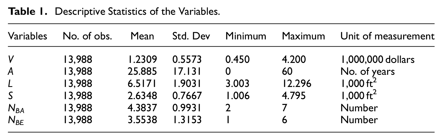
It can be seen that detached houses in Richmond sold for a considerable amount of money over our sample period, that is, they sold for an average of $1,230,900.

3. The Basic Models Using the Purchaser Perspective

Our fundamental problem is to decompose the value of a residential property into additive land and structure components. Our attempt to solve this imputation problem proceeds as follows. We assume initially that the total value of a property is equal to the floor space area of the structure, say S square feet, times the purchaser’s subjective valuation per square foot β _t during quarter t, plus the area of the land plot, say L square feet, times the purchaser’s subjective valuation per square foot α _t . We let t run from 1 to 44 where quarter 1 is the first quarter in 2008. Now think of a sample of properties of the same general type, which have sale prices or values V _tn in quarter t and structure and land areas, S _tn and L _tn , for n = 1, …, N(t) where N(t) is the number of sales in quarter t. Assume that these property values are equal to the sum of the land and structure values plus error terms ε _tn which we assume are independently normally distributed with zero means and constant variances. This leads to the following hedonic regression model for period t where the α _t and β _t are the parameters to be estimated in the regression:

$$V_{\mathrm{tn}}={\alpha }_t{L}_{\mathrm{tn}}+{\beta }_t{S}_{\mathrm{tn}}+{\epsilon }_{\mathrm{tn}};t=1,\dots ,44;n=1,\dots ,N\left(t\right)$$

(1)

Other papers that have suggested hedonic regression models that lead to additive decompositions of property values into land and structure components include Clapp (1980), Bostic et al. (2007), Francke and Vos (2004), Francke (2008, 167), Koev and Santos Silva (2008), and Rambaldi et al. (2011).

The hedonic regression model defined by Equation (1) applies to properties in the same general location and to structures of the same general quality. The parameter α _t can be interpreted as a quarter t average per unit price of land and the parameter β _t can be interpreted as a quarter t average per unit price of structures. The model defined by Equation (1) can accommodate residential properties that have no structure on them: S _tn is simply set equal to 0 for these properties. This is an advantage of our additive decomposition of property value into the sum of land and structure values.

It is likely that a purchaser’s valuation of the structure on the property declines as the age of the structure increases. Older structures will be worth less than newer structures due to the depreciation of the structure. Assuming that we have information on the age of the structure n at time t, say A(t, n), and assuming a geometric (or declining balance) depreciation model, a more realistic hedonic regression model than that defined by Equation (1) above is the following purchaser’s valuation model:

$$V_{\mathrm{tn}}={\alpha }_t{L}_{\mathrm{tn}}+{\beta }_t(1-\delta {)}^{A(t,n)}{S}_{\mathrm{tn}}+{\epsilon }_{\mathrm{tn}};t=1,\dots ,44;n=1,\dots ,N(t)$$

(2)

where the parameter δ reflects the net geometric depreciation rate as the structure ages one additional year.

In general, we would expect an annual net depreciation rate to be around 2% to 3% per year. This estimate of depreciation is regarded as a net depreciation rate because it is equal to a “true” gross structure depreciation rate less an average renovations appreciation rate. Since we do not have information on renovations and major repairs to a structure, our age variable will only pick up average gross depreciation less average real renovation expenditures.

Note that Equation (2) is now a nonlinear regression model whereas Equation (1) was a simple linear regression model. The period t imputed constant quality price of land is the estimated coefficient for the parameter α _t and the imputed price or marginal utility value of a unit of a newly built structure for period t is the estimate for β_t. The period t quantity of land for property n is L _tn and the period t quantity of structure for property n, expressed in equivalent quality adjusted units of a new structure, is (1 −δ)^A(t,n)S _tn where S _tn is the floor space area of the structure for property n in period t. It should be noted that a constant geometric depreciation rate may not provide an adequate description of depreciation in many situations where for example, some structures last for centuries. Thus more complex models of depreciation may have to be used in many situations.

Equation (2) is identical to the simplest version of the Builder’s Model that also attempts to decompose property value into land and structure components; see Diewert (2008, 2010, 2013), Diewert et al. (2011, 2015), Diewert and Shimizu (2015, 2016, 2020, 2022), and Burnett-Issacs et al. (2020) for materials on this model. The Builder’s Model sets the parameters β _t equal to a building construction cost index times a constant. This model can be justified for the sales of newly constructed houses but is less well justified for properties with older structures. Moreover, the Builder’s Model requires an appropriate exogenous construction cost index, which is typically difficult to find. The present model does not use a construction cost index; the β _t are estimated. Thus, the present model takes a consumer or purchaser perspective and could be called the Purchaser’s Model. See Rosen (1974) for a classification of hedonic models into supply and demand side models.

There is a major practical problem with the hedonic regression model defined by Equation (2): the multicollinearity problem. Experience has shown that it is usually not possible to estimate sensible land and structure prices in a hedonic regression like that defined by Equation (2) due to the multicollinearity between lot size and structure size; see Schwann (1998), Diewert (2010), and Diewert et al. (2011, 2015) on this problem. Thus in order to deal with the multicollinearity problem, we assumed that the forty-four structure valuation quarterly parameters β _t in Equation (2) can be described by twelve annual parameters, γ₁, γ₂, …, γ₁₂, as follows:

$$\begin{array}{c}\multicolumn{1}{c}{{\beta }_1={\gamma }_1;{\beta }_2=(3/4){\gamma }_1+(1/4){\gamma }_2;{\beta }_3=(1/2){\gamma }_1+(1/2){\gamma }_2;{\beta }_4=(1/4){\gamma }_1+(3/4){\gamma }_2;}\\ \multicolumn{1}{c}{{\beta }_5={\gamma }_2;{\beta }_6=(3/4){\gamma }_2+(1/4){\gamma }_3;{\beta }_7=(1/2){\gamma }_2+(1/2){\gamma }_3;{\beta }_8=(1/4){\gamma }_2+(3/4){\gamma }_3;}\\ \multicolumn{1}{c}{{\beta }_9={\gamma }_3;{\beta }_6=(3/4){\gamma }_3+(1/4){\gamma }_4;{\beta }_7=(1/2){\gamma }_3+(1/2){\gamma }_4;{\beta }_8=(1/4){\gamma }_3+(3/4){\gamma }_4;}\\ \multicolumn{1}{c}{...}\\ \multicolumn{1}{c}{{\beta }_{41}={\gamma }_{11};{\beta }_{42}=(3/4){\gamma }_{11}+(1/4){\gamma }_{12};{\beta }_{43}=(1/2){\gamma }_{11}+(1/2){\gamma }_{12};}\\ \multicolumn{1}{c}{{\beta }_{44}=(1/4){\gamma }_{11}+(3/4){\gamma }_{12};}\end{array}$$

(3)

Basically, we replaced the forty-four quarterly parameters β _t by a linear spline function with break points or knots at the beginning of each year. Thus, instead of estimating 44 β _t , we only estimated twelve annual parameters γ₁, …, γ₁₂. This specification of the structure valuation parameters has the effect of smoothing the β _t . More complex smoothing procedures could be used such as the Continuously Changing Coefficient smoothing procedure suggested by von Auer (2007), which is a form of polynomial smoothing. Other reasonable smoothing methods include the use of quadratic or cubic splines with endogenous break points. However, the present paper works with the above very simple model that could be the starting point for a better but more complex model (which might be difficult for National Statistical Offices to explain to the public).

An alternative strategy to solve the multicollinearity problem would be to smooth the α _t instead of the β _t . However, for a property with a new structure, the parameter β _t should be approximately equal to the per unit floor space area construction cost. Thus, for newly constructed houses, the movements in β _t should be approximately equal to the movements in an appropriate construction cost index. In general, construction cost indexes are not as volatile as land cost indexes, so we chose to smooth the β _t instead of the α _t .

Model 1 is defined by Equation (2) with the β _t defined by Equation (3). This model has forty-four quarterly land valuation or price parameters (the α_t), twelve annual structure valuation parameters (γ₁, …, γ₁₂) and one (net) geometric structure depreciation rate δ for a total of fifty-seven parameters with 13,988 observations. The lowest number of sales in a quarter was 92 and the highest number was 631. The average number of sales in a quarter was 317.9. The R² (between the observed values and the predicted values) was .8207, which we regarded as satisfactory for such a simple model. The estimates for the annual structure price parameters γ₁*, …, γ₁₂* were 0.233, 0.223, 0.260, 0.285, 0.314, 0.330, 0.321, 0.317, 0.400, 0.425, 0.411, and 0.430. Using these estimates for γ₁* to γ₁₂*, definitions Equation (3) were used to form the quarterly structure prices, β _t * for t = 1, …, 44. The estimated depreciation rate δ* was 1.98% per year. Land prices grew from α₁* = $57.34 per ft² in the first quarter of 2008 to α₄₄* = $149.08 per ft² in the last quarter of 2018, a 2.60-fold increase over the sample period.

Structure prices grew from β₁* = $233.45 per ft² in the first quarter of 2008 to β₄₄* = $425.60 per ft² in the last quarter of 2018, a 1.82-fold increase over the sample period. From the Altus Group (2015) Construction Cost Guide for 2015, we find the following range of house construction costs per square foot for the Vancouver area: Speculative Basic Quality: $100 to $165; Speculative Medium Quality: $165 to $225; Speculative High Quality: $225 to $350; Custom Built: $400 to $1,000. It can be seen that our estimated valuations for units of structure are within the range of construction costs for the Greater Vancouver area. The above ranges also indicate the difficulty in obtaining a representative construction cost index for detached houses.

The estimated land and structure valuation coefficients, α _t * and β _t *, were turned into the land and structure price indexes for Model 1, $P_{L1}^t\equiv {\alpha }_t^{*}/{\alpha }_1^{*}$ and $P_{S1}^t\equiv {\beta }_t^{*}/{\beta }_1^{*}$ and these indexes are listed in Table 3 below.

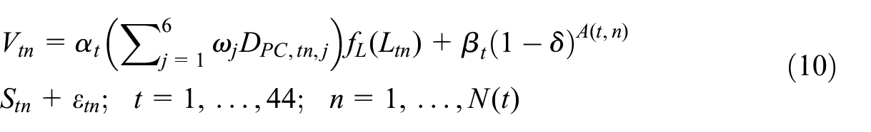
In order to take into account possible neighborhood effects on the price of land, we introduced (forward sortation area) postal code dummy variables, D_PC, _tn , _j , into the hedonic regression defined by Equations (2) and (3). The number of observations over the sample period in the six postal code neighborhoods are as follows: 468, 1,041, 1,038, 2,930, 4,404, and 4,107. These six dummy variables are defined as follows: for t = 1, …, 44; n = 1, …, N(t); j = 1, …, 6:

$$\begin{array}{c}\multicolumn{1}{c}{D_{\mathrm{PC},\mathrm{tn},j}\equiv 1\mathrm{if}\mathrm{observation}n\mathrm{in}\mathrm{period}t\mathrm{is}\mathrm{in}\mathrm{Postal}\mathrm{Code}j\mathrm{of}\mathrm{Richmond};}\\ \multicolumn{1}{c}{\equiv 0\mathrm{if}\mathrm{observation}n\mathrm{in}\mathrm{period}t\mathrm{is}\mathrm{not}\mathrm{in}\mathrm{Postal}\mathrm{Code}j\mathrm{of}\mathrm{Richmond}.}\end{array}$$

(4)

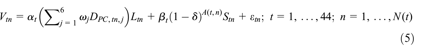
We now modify the model defined by Equations (2) and (3) to allow the level of the quality of land to differ across the six postal-code areas in Richmond. The new nonlinear regression model is defined by Equations (3) and (5):

$$V_{\mathrm{tn}}={\alpha }_t\left(\sum _{j=1}^6{\omega }_j{D}_{\mathrm{PC},\mathrm{tn},j}\right)L_{\mathrm{tn}}+{\beta }_t{(1-\delta )}^{A(t,n)}{S}_{\mathrm{tn}}+{\epsilon }_{\mathrm{tn}};t=1,\dots ,44;n=1,\dots ,N(t)$$

(5)

Comparing the models defined by Equations (2) and (5), it can be seen that we have added an additional six neighborhood relative land valuation parameters, ω₁, …,ω₆, to the model defined by Equation (2). The higher is ω₁, the greater is the utility of owning a square foot of land in Postal Code 1 relative to owning a square foot of land in the other Postal Codes. However, looking at Equation (5), it can be seen that the forty-four land aggregate price level parameters (the α _t ) and the six location parameters (the ω _j ) cannot all be identified. Thus, we need to impose at least one identifying normalization on these parameters. We chose the following normalization:

$${\omega }_1\equiv 1$$

(6)

Model 2 defined by Equations (3), (5), and (6) has five additional parameters compared to Model 1. Note that if we initially set all of the ω _j equal to unity, Model 2 collapses down to Model 1. We made use of this fact in running our sequence of nonlinear regressions. Our models are nested so that we can use the final parameter estimates from a previous model as starting parameter values in the next model’s nonlinear regression. In order to obtain sensible parameter estimates in our final (quite complex) nonlinear regression model, we nested our models so that each new model contained by previous model as a special case. This enabled us to use the final estimated coefficients from the previous model as starting values for the same coefficients in the subsequent model. We structured the models and the starting coefficients so that the initial log likelihood for the present model was equal to the final log likelihood for the previous model. This is a useful check on our codes. We used both Shazam and RStudio to perform the nonlinear regressions; see White (2004).

The final log likelihood (LL) for Model 2 was an improvement of 1,257.586 over the final LL for Model 1 (for adding five new neighborhood parameters) which, of course, is a highly significant increase. The R² increased to .8512 from the previous model R² of .8207. The new estimated depreciation rate turned out to be 0.0184 or 1.84% per year. The price of land increased 2.90 fold and the price of structures increased 1.87 fold over the sample period. The Model 2 land and structure price indexes, $P_{L2}^t\equiv {\alpha }_t^{*}/{\alpha }_1^{*}$ and $P_{S2}^t\equiv {\beta }_t^{*}/{\beta }_1^{*}$ , are listed in Table 3 below. The estimated postal code coefficients ω₂*, …, ω₆* were 1.1467, 1.9539, 1.7260, 2.0055, and 1.9576.

In our next model, we introduced some nonlinearities into the pricing of the land area for each property. As mentioned in Section 2, the land plot areas in our sample of properties ran from 3,000 to 12,300 ft². Up to this point, we have assumed that land plots in the same neighborhood are valued by purchasers at a constant marginal utility per square foot of lot area. However, it is likely that there is some nonlinearity in this valuation schedule; for example, it is likely that large lots are valued at a marginal utility that is below the marginal utility of medium sized lots. In order to capture this nonlinearity, we initially divided up our 13,988 observations into five groups of observations based on their lot size. The Group 1 properties had lots less than 4,500 ft², the Group 2 properties had lots greater than or equal to 4,500 ft² and less than 6,000 ft², the Group 3 properties had lots greater than or equal to 6,000 ft² and less than 7,500 ft², the Group 4 properties had lots greater than or equal to 7,500 ft² and less than 9,000 ft², and the Group 5 properties had lots greater than or equal to 9,000 ft². The number of properties falling into each group were 2,927, 2,397, 4,236, 3,162, and 1,266. The use of linear splines to model land prices as a function of lot size was first used by Diewert et al. (2011). The four land values L _t (in units of thousand ft²) used to define the boundaries of the above five groups are defined as follows:

$$L_1\equiv 4.5;L_2\equiv 6;L_3\equiv 7.5;L_4\equiv 9.$$

(7)

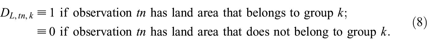
For each observation n in period t, we define the five land dummy variables, D_L, _tn , _k , for k = 1, …, 5 as follows:

$$\begin{array}{c}\multicolumn{1}{c}{D_{L,\mathrm{tn},k}\equiv 1\mathrm{if}\mathrm{observation}\mathrm{tn}\mathrm{has}\mathrm{land}\mathrm{area}\mathrm{that}\mathrm{belongs}\mathrm{to}\mathrm{group}k;}\\ \multicolumn{1}{c}{\equiv 0\mathrm{if}\mathrm{observation}\mathrm{tn}\mathrm{has}\mathrm{land}\mathrm{area}\mathrm{that}\mathrm{does}\mathrm{not}\mathrm{belongs}\mathrm{to}\mathrm{group}k.}\end{array}$$

(8)

These dummy variables are used in the definition of the following piecewise linear function of L _tn , f _L (L _tn ), defined as follows:

$$\begin{array}{c}\multicolumn{1}{c}{f_L\left(L_{\mathrm{tn}}\right)\equiv D_{L,\mathrm{tn},1}{\lambda }_1{L}_{\mathrm{tn}}+D_{L,\mathrm{tn},2}[{\lambda }_1{L}_1+{\lambda }_2(L_{\mathrm{tn}}-L_1)]}\\ \multicolumn{1}{c}{+D_{L,\mathrm{tn},3}[{\lambda }_1{L}_1+{\lambda }_2(L_2-L_1)+{\lambda }_3(L_{\mathrm{tn}}-L_2)]}\\ \multicolumn{1}{c}{+D_{L,\mathrm{tn},4}[{\lambda }_1{L}_1+{\lambda }_2(L_2-L_1)+{\lambda }_3(L_3-L_2)+{\lambda }_4(L_{\mathrm{tn}}-L_3)]}\\ \multicolumn{1}{c}{+D_{L,\mathrm{tn},5}[{\lambda }_1{L}_1+{\lambda }_2(L_2-L_1)+{\lambda }_3(L_3-L_2)+{\lambda }_4(L_4-L_3)+{\lambda }_5(L_{\mathrm{tn}}-L_4)]}\end{array}$$

(9)

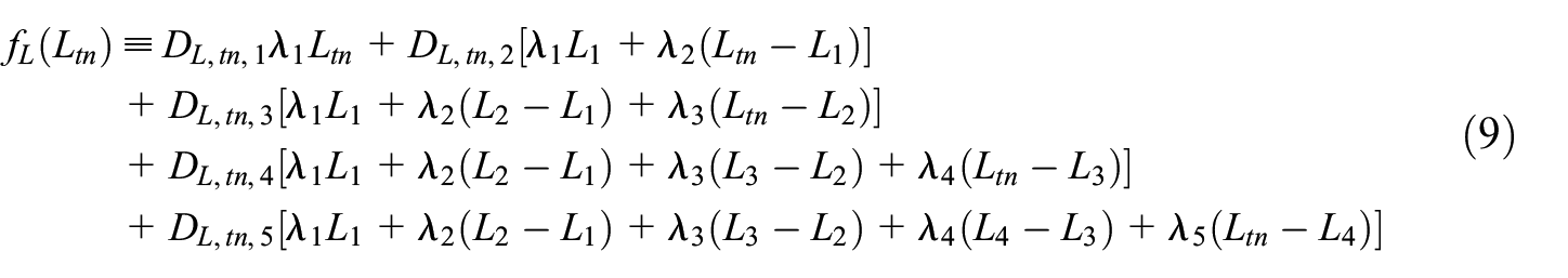
where the λ _k are unknown parameters, and the L _t are defined by Equation (7). The function f _L (L _tn ) defines a relative valuation function for the land area of a property as a function of the plot area. Basically, we are assuming that all purchasers of the residential properties in scope have the land utility function u(L _tn ) for property n in quarter t equal to (Σ⁶ _{j =1}ω_jD_PC, _tn , _j )f _L (L _tn ) and the corresponding structure utility function U(S _tn ) for property n in quarter t is equal to (1 −δ)^A(t,n)S _tn . These are very strong assumptions.

The new nonlinear regression model is the following one:

$$\begin{array}{c}\multicolumn{1}{c}{V_{\mathrm{tn}}={\alpha }_t\left(\sum _{j=1}^6{\omega }_j{D}_{\mathrm{PC},\mathrm{tn},j}\right)f_L(L_{\mathrm{tn}})+{\beta }_t{(1-\delta )}^{A(t,n)}}\\ \multicolumn{1}{c}{S_{\mathrm{tn}}+{\epsilon }_{\mathrm{tn}};t=1,\dots ,44;n=1,\dots ,N(t)}\end{array}$$

(10)

Comparing the models defined by Equations (5) and (10), it can be seen that we have added an additional five land plot size parameters, λ₁, …,λ₅, to the model defined by Equation (5). However, looking at Equations (9) and (10), it can be seen that the forty-four land price parameters (the α _t ), the six postal code parameters (the ω _j ), and the five land plot size parameters (the λ _k ) cannot all be identified. Thus we impose the following identification normalizations on the parameters for Model 3 defined by Equations (3), (10), and (11):

$${\omega }_1\equiv 1;{\lambda }_1\equiv 1.$$

(11)

Note that if we set all of the λ _k equal to unity, Model 3 collapses down to Model 2. The final log likelihood for Model 3 was an improvement of 1,076.866 over the final log likelihood for Model 2 (for adding four new lot size parameters) which is a highly significant increase. The R² increased to .8683 from the previous model R² of .8512. The new estimated geometric depreciation rate for structures turned out to be 0.0328 or 3.28% per year. The price of land increased 2.37 fold over the sample period while the price of structures increased 1.84 fold. Thus the new model has given rise to somewhat different land prices and the new depreciation rate is considerably higher than the depreciation rates in Models 1 and 2. The sequence of marginal utility land quality adjustment factors generated by this model are as follows: λ₁ = 1 (imposed), λ₂* = 0.26174, λ₃* = 0.45155, λ₄* = 0.64362, and λ₅* = 0.25290. Thus, the marginal utility land valuations as functions of lot size are not monotonic. The Model 3 land and structure price indexes, $P_{L3}^t\equiv {\alpha }_t^{*}/{\alpha }_1^{*}$ and $P_{S3}^t\equiv {\beta }_t^{*}/{\beta }_1^{*}$ , are listed in Table 3 below.

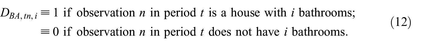
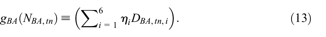
For our final model, we introduced bathroom and bedroom variables into the hedonic regression as variables that could affect the quality of the structure on a property. The number of bathrooms in our sample ranged from one to six bathrooms. The number of observations in each of the six bathroom cells was 419, 2,236, 5,664, 2,243, 1,700, 1,726. Thus define the following six dummy variables, D _BA , _tn,i : for t = 1, …, 44; n = 1, …, N(t); i = 1, …, 6:

$$\begin{array}{c}\multicolumn{1}{c}{D_{\mathrm{BA},\mathrm{tn},i}\equiv 1\mathrm{if}\mathrm{observation}n\mathrm{in}\mathrm{period}t\mathrm{is}\mathrm{a}\mathrm{house}\mathrm{with}i\mathrm{bathrooms};}\\ \multicolumn{1}{c}{\equiv 0\mathrm{if}\mathrm{observation}n\mathrm{in}\mathrm{period}t\mathrm{does}\mathrm{not}\mathrm{have}i\mathrm{bathrooms}.}\end{array}$$

(12)

We used the bathroom dummy variables defined above in order to define the following bathroom quality adjustment function, g_BA(N _BA , _tn ), as follows:

$$g_{\mathrm{BA}}\left(N_{\mathrm{BA},\mathrm{tn}}\right)\equiv \left(\sum _{i=1}^6{\eta }_i{D}_{\mathrm{BA},\mathrm{tn},i}\right).$$

(13)

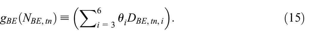
Finally, we introduced the number of bedrooms into the hedonic regression. The number of bedrooms in our sample ranged from two to seven bedrooms. The number of observations in each of the six bedroom cells was 118, 2,832, 4,413, 5,062, 1,316, 247. Define the following six dummy variables, D _BE , _tn,i , for t = 1, …, 44; n = 1, …, N(t); i = 2, 3, …, 7:

$$\begin{array}{c}\multicolumn{1}{c}{D_{\mathrm{BE},\mathrm{tn},i}\equiv 1\mathrm{if}\mathrm{observation}n\mathrm{in}\mathrm{period}t\mathrm{is}\mathrm{a}\mathrm{house}\mathrm{with}i\mathrm{bedrooms};}\\ \multicolumn{1}{c}{\equiv 0\mathrm{if}\mathrm{observation}n\mathrm{in}\mathrm{period}t\mathrm{does}\mathrm{not}\mathrm{have}i\mathrm{bedrooms}.}\end{array}$$

(14)

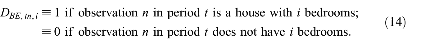
There were not a sufficient number of properties that had only two bedrooms (118) or had seven bedrooms (247), so we combined cell 2 with cell 3 and combined cell 7 with cell 6. Thus we ended up with four cells and four dummy variables of the form D _BE , _tn,i defined by Equation (14). We use the bedroom dummy variables defined above in order to define the following bedroom quality adjustment function, g_BE(N _BE , _tn ):

$$g_{\mathrm{BE}}\left(N_{\mathrm{BE},\mathrm{tn}}\right)\equiv \left(\sum _{i=3}^6{\theta }_i{D}_{\mathrm{BE},\mathrm{tn},i}\right).$$

(15)

The new nonlinear regression model is the following one:

$$\begin{array}{c}\multicolumn{1}{c}{V_{\mathrm{tn}}={\alpha }_t\left(\sum _{j=1}^6{\omega }_j{D}_{\mathrm{PC},\mathrm{tn},j}\right)f_L(L_{\mathrm{tn}})+{\beta }_t{(1-\delta )}^{A(t,n)}{g}_{\mathrm{BA}}\left(N_{\mathrm{BA},\mathrm{tn}}\right)g_{\mathrm{BE}}\left(N_{\mathrm{BE},\mathrm{tn}}\right)S_{\mathrm{tn}}+{\epsilon }_{\mathrm{tn}};}\\ \multicolumn{1}{c}{t=1,\dots ,44;n=1,\dots ,N(t)}\end{array}$$

(16)

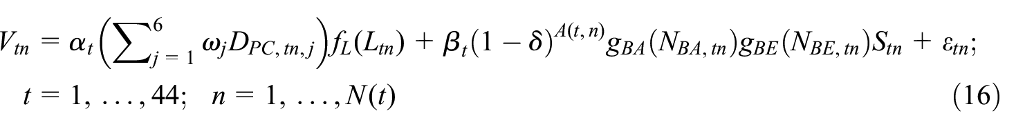
The utility function u(L) that adjusts the quantity of land for observation n in period t, L _tn , into quality adjusted land is u(L _tn ) ≡ (Σ⁶_j=1ω_jD_PC, _tn,j )f _L (L _tn ) ≡L _tn * and the utility function U(S _tn ) that adjusts the quantity of structures for observation n in period t, S _tn , into quality adjusted structures is U(S _tn ) ≡ (1 −δ)^A(t,n)g _BA (N _BA , _tn )g _BE (N _BE , _tn )S_tn≡ S_tn*. McMillen’s (2003) consumer-oriented approach to property hedonics assumed that all purchasers have Cobb-Douglas preferences over combinations of L _tn * and S _tn * whereas we assume that purchasers have separate preference functions, u(L) and U(S), for land and structures.

Comparing the models defined by Equations (10) and (16), it can be seen that we have added an additional six bathroom parameters η _i and four additional bedroom parameters θ _i to the model defined by Equation (5). However, it can be seen that the forty-four land price parameters (the α _t ), the six postal code parameters (the ω _j ), the five land plot size parameters (the λ _k ), the six bathroom parameters (the η _k ), and the four bedroom parameters (the θ _k ) cannot all be identified. Thus we impose the following identification normalizations on the parameters for Model 4 defined by Equations (3), (10), (13), (15), (16), and (17):

$${\omega }_1\equiv 1;{\lambda }_1\equiv 1;{\eta }_1=1;{\theta }_3=1.$$

(17)

There are a total of seventy-four unknown parameters in Model 4. Note that if we set all of the η _k and θ _k equal to 1, then Model 4 collapses down to Model 3.

The final log likelihood for Model 4 was an improvement of 264.781 over the final log likelihood for Model 3 (for adding eight new bathroom and bedroom parameters). The R² increased to .8732 from the previous model R² of .8633. The estimated geometric depreciation rate was δ* = 0.0281 or 2.81% per year. Using this model, the price of land increased 2.46 fold which is an increase over the 2.37 fold increase that occurred in Model 3. The price of structures increased 1.74 fold. The Model 4 land and structure price indexes, $P_{L4}^t\equiv {\alpha }_t^{*}/{\alpha }_1^{*}$ and $P_{S4}^t\equiv {\beta }_t^{*}/{\beta }_1^{*}$ , are listed in Table 3.

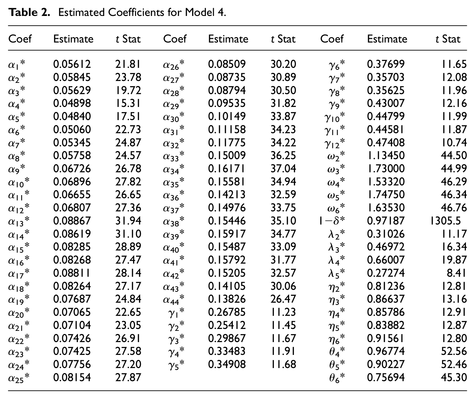
The estimated coefficients for Model 4 are listed in Table 2.

Table 2.

Estimated Coefficients for Model 4.

Coef	Estimate	t Stat	Coef	Estimate	t Stat	Coef	Estimate	t Stat
α1*	0.05612	21.81	α26*	0.08509	30.20	γ6*	0.37699	11.65
α2*	0.05845	23.78	α27*	0.08735	30.89	γ7*	0.35703	12.08
α3*	0.05629	19.72	α28*	0.08794	30.50	γ8*	0.35625	11.96
α4*	0.04898	15.31	α29*	0.09535	31.82	γ9*	0.43007	12.16
α5*	0.04840	17.51	α30*	0.10149	33.87	γ10*	0.44799	11.99
α6*	0.05060	22.73	α31*	0.11158	34.23	γ11*	0.44581	11.87
α7*	0.05345	24.87	α32*	0.11775	34.22	γ12*	0.47408	10.74
α8*	0.05758	24.57	α33*	0.15009	36.25	ω2*	1.13450	44.50
α9*	0.06726	26.78	α34*	0.16171	37.04	ω3*	1.73000	44.99
α10*	0.06896	27.82	α35*	0.15581	34.94	ω4*	1.53320	46.29
α11*	0.06655	26.65	α36*	0.14213	32.59	ω5*	1.74750	46.34
α12*	0.06807	27.36	α37*	0.14976	33.75	ω6*	1.63530	46.76
α13*	0.08867	31.94	α38*	0.15446	35.10	1−δ*	0.97187	1305.5
α14*	0.08619	31.10	α39*	0.15917	34.77	λ2*	0.31026	11.17
α15*	0.08285	28.89	α40*	0.15487	33.09	λ3*	0.46972	16.34
α16*	0.08268	27.47	α41*	0.15792	31.77	λ4*	0.66007	19.87
α17*	0.08811	28.14	α42*	0.15205	32.57	λ5*	0.27274	8.41
α18*	0.08264	27.17	α43*	0.14105	30.06	η2*	0.81236	12.81
α19*	0.07687	24.84	α44*	0.13826	26.47	η3*	0.86637	13.16
α20*	0.07065	22.65	γ1*	0.26785	11.23	η4*	0.85786	12.91
α21*	0.07104	23.05	γ2*	0.25412	11.45	η5*	0.83882	12.87
α22*	0.07426	26.91	γ3*	0.29867	11.67	η6*	0.91561	12.80
α23*	0.07425	27.58	γ4*	0.33483	11.91	θ4*	0.96774	52.56
α24*	0.07756	27.20	γ5*	0.34908	11.68	θ5*	0.90227	52.46
α25*	0.08154	27.87				θ6*	0.75694	45.30

The land price indexes generated by Models 1 to 4, P _{L 1} ^t , P _{L 2} ^t , P _{L 3} ^t , P _{L 4} ^t , and the corresponding structure prices, P _{S 1} ^t , P _{S 2} ^t , P _{S 3} ^t , P _{S 4} ^t , are listed in Table 3.

Table 3.

Land and Structure Price Indexes for Models 1 to 4.

Quarter t	P L 1 t	P L 2 t	P L 3 t	P L 4 t	P S 1 t	P S 2 t	P S 3 t	P S 4 t
1	1.00000	1.00000	1.00000	1.00000	1.00000	1.00000	1.00000	1.00000
2	1.03429	1.04492	1.03623	1.04157	0.98862	0.98534	0.98834	0.98718
3	1.02270	1.01530	1.00517	1.00302	0.97724	0.97067	0.97668	0.97436
4	0.81897	0.83256	0.88105	0.87275	0.96586	0.95601	0.96502	0.96155
5	0.86209	0.85270	0.87102	0.86247	0.95448	0.94134	0.95336	0.94873
6	0.88388	0.87278	0.90375	0.90161	0.99399	0.98373	0.99908	0.99031
7	0.92769	0.92302	0.95703	0.95241	1.03349	1.02611	1.04480	1.03189
8	0.99921	0.99533	1.01975	1.02594	1.07299	1.06849	1.09052	1.07347
9	1.21342	1.20019	1.18039	1.19856	1.11249	1.11088	1.13625	1.11505
10	1.25935	1.26292	1.21023	1.22886	1.13943	1.13169	1.17369	1.14880
11	1.20008	1.20113	1.17133	1.18592	1.16637	1.15251	1.21113	1.18255
12	1.22499	1.22994	1.19849	1.21292	1.19331	1.17333	1.24857	1.21630
13	1.67840	1.71518	1.54366	1.58005	1.22025	1.19415	1.28602	1.25006
14	1.60468	1.64631	1.49572	1.53585	1.25180	1.21649	1.30086	1.26336
15	1.51471	1.56576	1.44633	1.47636	1.28334	1.23883	1.31571	1.27665
16	1.50904	1.54416	1.44676	1.47328	1.31489	1.26116	1.33055	1.28995
17	1.62407	1.69986	1.53951	1.57003	1.34643	1.28350	1.34540	1.30325
18	1.49395	1.56524	1.44804	1.47258	1.36301	1.30903	1.38039	1.32930
19	1.40415	1.42607	1.35843	1.36977	1.37959	1.33456	1.41537	1.35535
20	1.23604	1.23821	1.23902	1.25885	1.39616	1.36010	1.45036	1.38140
21	1.26681	1.27912	1.24682	1.26590	1.41274	1.38563	1.48535	1.40745
22	1.34289	1.34866	1.30788	1.32329	1.40347	1.37171	1.46370	1.38882
23	1.31616	1.34908	1.30660	1.32308	1.39420	1.35780	1.44206	1.37019
24	1.36682	1.39764	1.35620	1.38200	1.38494	1.34388	1.42041	1.35156
25	1.44230	1.48147	1.41957	1.45299	1.37567	1.32996	1.39876	1.33293
26	1.54831	1.57025	1.48575	1.51619	1.37084	1.33152	1.39324	1.33221
27	1.56188	1.60358	1.52464	1.55647	1.36601	1.33308	1.38771	1.33148
28	1.59471	1.62161	1.53541	1.56704	1.36118	1.33464	1.38219	1.33076
29	1.77298	1.77770	1.65843	1.69898	1.35635	1.33620	1.37666	1.33003
30	1.84837	1.88539	1.75741	1.80854	1.44593	1.40812	1.45738	1.39893
31	2.01062	2.06941	1.92450	1.98833	1.53551	1.48003	1.53810	1.46783
32	2.14408	2.21320	2.03030	2.09810	1.62508	1.55194	1.61882	1.53672
33	2.79336	2.89867	2.56353	2.67442	1.71466	1.62386	1.69953	1.60562
34	3.07233	3.18879	2.76067	2.88151	1.74112	1.66125	1.72084	1.62234
35	2.90058	3.01479	2.67023	2.77631	1.76758	1.69865	1.74214	1.63906
36	2.56677	2.72080	2.43911	2.53261	1.79404	1.73605	1.76345	1.65579
37	2.79210	2.84140	2.54910	2.66850	1.82050	1.77345	1.78475	1.67251
38	2.87762	2.93606	2.64755	2.75237	1.80549	1.78428	1.77036	1.67048
39	2.99580	2.99926	2.71455	2.83628	1.79049	1.79511	1.75597	1.66844
40	2.89693	2.86556	2.64936	2.75963	1.77548	1.80595	1.74158	1.66640
41	2.99874	2.95208	2.71392	2.81395	1.76047	1.81678	1.72719	1.66436
42	2.85707	2.77317	2.61565	2.70945	1.78135	1.83431	1.76513	1.69075
43	2.68382	2.57442	2.43619	2.51334	1.80223	1.85184	1.80306	1.71714
44	2.59995	2.49497	2.37305	2.46374	1.82311	1.86937	1.84099	1.74353

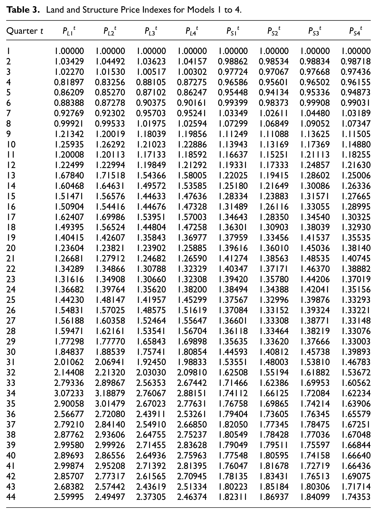
Figure 1 plots the four land price indexes and Figure 2 plots the four structure price indexes.

Figure 1.

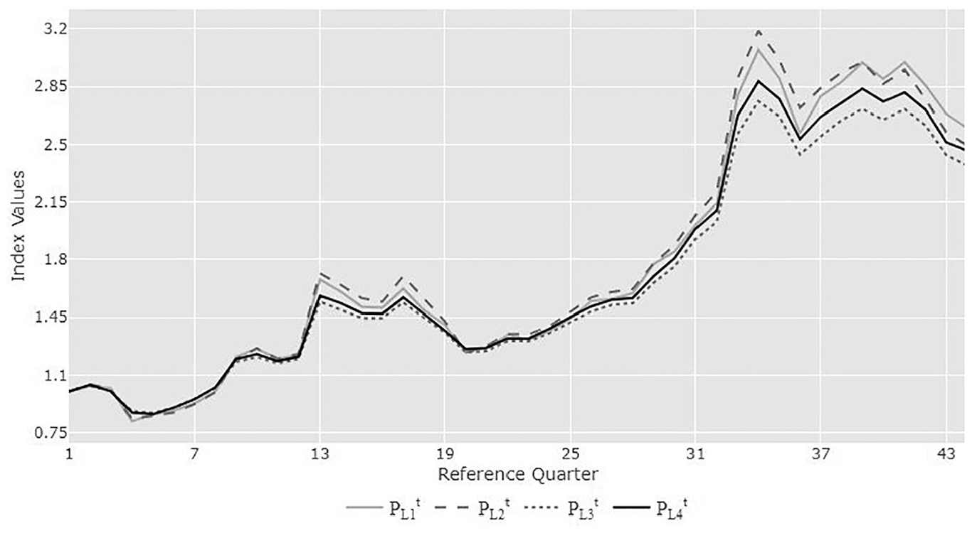
Land price indexes form Models 1 to 4.

Figure 2.

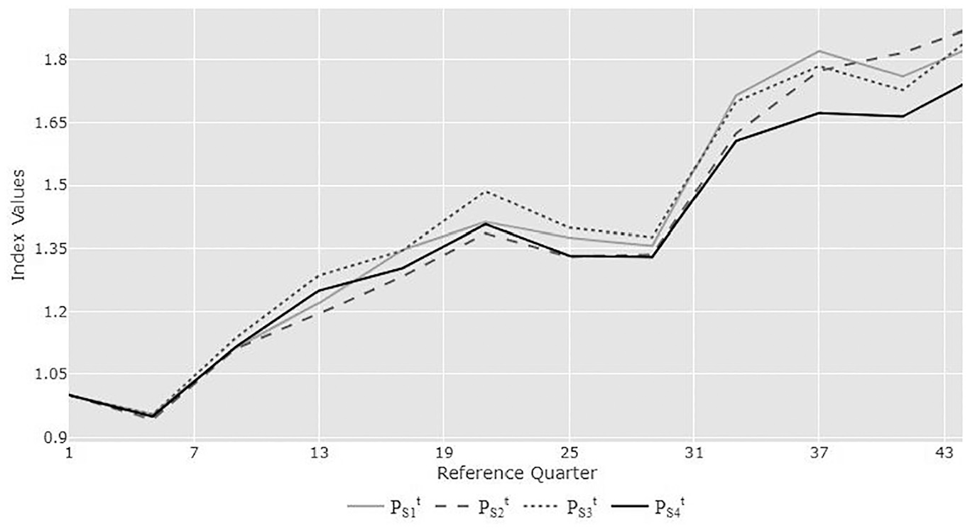
Structure price indexes form Models 1 to 4.

It can be seen that the different models generate substantially different land and structure price indexes at times, although they all pick up the same trends. We prefer the Model 4 indexes since this model fits the data best.

In the following section, we will use the results from Models 1 to 4 to construct overall property price indexes.

4. Property Price Indexes for the Purchasers' Models

The previous section showed how the value of property n in period t, V _tn , could be decomposed into the sum of a land component, a structure component, and an error term. In the case of Model 1, the land component was equal to α _t *L _tn and the structure component was equal to β _t *(1 −δ*)^A(t,n)S _tn . In the present section, we show how the various decompositions of property value can be aggregated to give us overall property price indexes for Richmond.

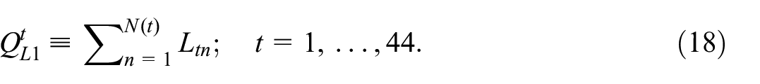
Using the estimated coefficients from Model 1, quarter t aggregate land Q_L1 ^t is defined as the sum of the land that was purchased in quarter t:

$$Q_{L1}^t\equiv \sum _{n=1}^{N(t)}{L}_{\mathrm{tn}};t=1,\dots ,44.$$

(18)

The corresponding aggregate quarter t predicted land price is defined as follows:

$$P_{L1}^t\equiv {\alpha }_t^{*};t=1,\dots ,44.$$

(19)

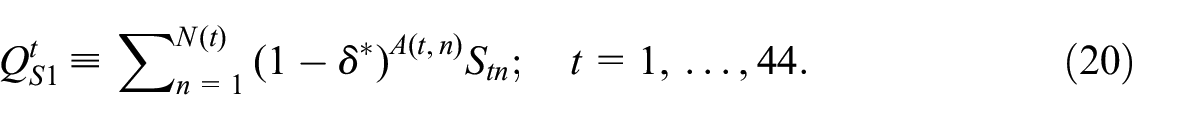
The Model 1 quarter t constant quality aggregate structure quantity is defined as the following sum:

$$Q_{S1}^t\equiv \sum _{n=1}^{N(t)}{(1-{\delta }^{*})}^{A(t,n)}{S}_{\mathrm{tn}};t=1,\dots ,44.$$

(20)

The corresponding constant quality aggregate quarter t structure price is defined as follows:

$$P_{S1}^t\equiv {\beta }_t^{*};t=1,\dots ,44.$$

(21)

where the β _t * are defined in terms of the estimated annual structure prices γ₁*, …, γ₁₂* for Model 1 using Equation (3).

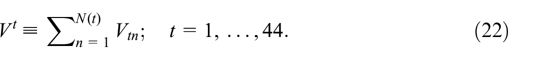
Define the quarter t total property value V ^t by summing over the individual quarter t transactions, V _tn :

$$V^t\equiv \sum _{n=1}^{N(t)}{V}_{\mathrm{tn}};t=1,\dots ,44.$$

(22)

Quarter t predicted aggregate property value V ^t* is defined as P _{L 1} ^t Q _{L 1} ^t plus P _{S 1} ^t Q _{S 1} ^t for t = 1, …, 44. However, due to the error terms in the hedonic regression that defined Model 1, V ^t* will not equal V ^t . In order to make the predicted value of property transacted in quarter t equal to the actual quarter t property value, we will not use definitions Equation (18) to define the Q _{L 1}^t; instead, we will use the following definitions:

$$Q_{L1}^t\equiv [V^t-P_{S1}^t{Q}_{S1}^t]/P_{L1}^t;t=1,\dots ,44.$$

(23)

If the fits in the various nonlinear regression models in the previous section are poor, the use of definitions Equation (23) will tend to make the aggregate land quantity levels more volatile than those produced by the original definitions Equation (18).

We use definitions Equations (19), (20), (21), and (23) to define preliminary values for P _{L 1} ^t , Q _{L 1} ^t , P _{S 1} ^t , and Q _{S 1} ^t for t = 1, …, 44. Finally, we normalize the price indexes P _{L 1} ^t and P _{S 1} ^t to equal one for t = 1 and normalize the companion quantity indexes (in the opposite direction) so that aggregate land and structure values remain unchanged for each quarter. In an abuse of notation, we denote the normalized series by P _{L 1} ^t , Q _{L 1} ^t , P _{S 1} ^t , and Q _{S 1} ^t for t = 1, …, 44. The Model 1 aggregate normalized price series P _{L 1} ^t and P _{S 1} ^t are listed in Table 3 and the corresponding normalized quantity series Q _{L 1} ^t and Q _{S 1} ^t are listed in Table 4.

Table 4.

Land and Structure Quantity Levels for Models 1 to 4.

Quarter t	Q L 1 t	Q L 2 t	Q L 3 t	Q L 4 t	Q S 1 t	Q S 2 t	Q S 3 t	Q S 4 t
1	141.53	135.005	188.209	173.795	151.965	158.486	105.282	119.696
2	131.37	124.668	173.552	160.044	144.554	150.726	100.113	113.543
3	52.77	51.163	71.288	65.768	60.298	62.794	42.226	48.167
4	36.13	34.093	47.084	43.531	41.941	43.634	29.653	33.391
5	81.64	79.810	111.817	103.599	100.252	104.127	72.038	80.868
6	176.21	170.935	241.171	222.679	204.673	213.473	141.358	159.969
7	195.15	187.607	259.380	239.982	220.005	229.261	153.310	174.291
8	133.50	128.019	176.185	163.026	152.168	158.393	107.287	120.552
9	175.83	170.411	233.271	215.810	184.458	192.675	126.041	143.405
10	143.56	137.832	193.293	178.448	154.709	161.710	104.924	119.942
11	114.58	110.603	153.177	141.401	121.782	127.286	82.672	94.590
12	147.18	142.351	195.785	181.193	156.201	163.299	105.754	120.788
13	227.25	218.369	297.908	275.783	208.539	218.853	136.871	160.103
14	140.00	134.499	185.784	171.672	134.780	141.349	88.783	102.673
15	103.73	99.545	138.485	128.223	111.268	116.277	75.711	86.638
16	78.59	76.366	105.924	97.874	78.014	81.867	51.048	59.671
17	102.71	98.268	139.563	128.786	107.128	112.199	71.496	83.522
18	86.53	82.408	116.364	107.333	95.951	100.129	66.329	76.735
19	59.60	58.166	81.625	75.493	70.561	73.493	49.561	57.271
20	56.75	55.499	77.603	71.686	67.782	70.631	47.321	53.960
21	80.95	77.762	111.110	102.261	92.286	96.318	63.550	73.519
22	124.95	121.465	170.552	157.698	138.606	144.719	95.146	110.632
23	126.76	121.347	171.812	158.713	148.484	154.772	103.579	119.594
24	98.81	95.489	132.600	122.551	118.404	123.206	83.921	95.940
25	134.15	129.474	178.659	165.268	149.892	156.302	104.428	119.703
26	146.60	142.157	198.753	183.642	153.352	160.709	101.857	119.181
27	145.80	139.435	193.142	178.840	163.965	171.110	113.300	130.186
28	119.71	115.220	157.557	146.153	124.379	129.891	85.579	98.570
29	187.02	182.082	249.463	230.943	200.133	209.060	137.521	158.393
30	247.04	238.514	326.199	302.158	252.441	264.136	170.416	196.696
31	187.82	181.143	246.991	228.912	193.092	202.208	129.249	149.187
32	177.00	171.609	234.840	217.547	184.157	192.647	124.774	144.689
33	217.82	210.400	285.066	264.114	198.800	209.029	128.586	151.318
34	191.86	184.719	256.132	237.050	193.206	202.742	127.113	149.646
35	78.22	74.951	103.352	95.664	81.785	85.646	54.800	64.580
36	59.79	55.874	78.241	72.267	61.474	64.365	41.353	48.762
37	102.33	99.183	139.589	128.840	115.819	121.089	78.856	91.331
38	146.94	140.769	196.039	181.423	163.337	170.616	112.243	130.735
39	82.77	80.082	110.898	102.635	87.907	92.005	59.402	68.474
40	75.01	72.567	100.447	92.999	84.441	88.189	58.046	66.352
41	63.41	61.041	85.594	79.062	70.874	74.160	47.844	55.549
42	76.62	74.545	103.335	95.688	91.223	95.227	62.950	72.240
43	57.56	56.580	78.712	72.756	68.612	71.533	47.904	55.481
44	37.89	37.266	51.542	47.614	42.901	44.798	29.554	34.077

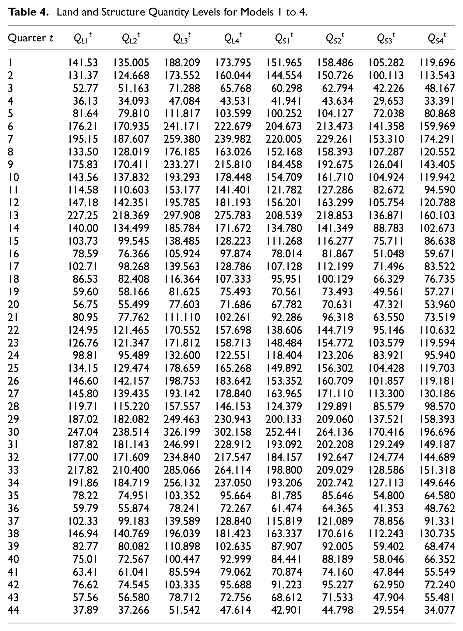
The same strategy for forming aggregate price and quantity indexes for the aggregate land and structure was followed using the results of Models 2 to 4. The preliminary constant quality land and structure price levels for quarter t were defined using the estimated coefficients from the relevant regression for the α _t * and the β _t * and using definitions Equations (20) and (23) in order to define the corresponding Model j constant quality quarter t structure and land levels, Q _Sj ^t and Q _Lj ^t . However, Model 4 used a different definition for Q _{S 4} ^t instead of using definition Equation (20). The Model 4 counterpart definitions to definitions Equation (20) are the following:

$$Q_{S4}^t\equiv \sum _{n=1}^{N(t)}{(1-{\delta }^{*})}^{A(t,n)}{g}_{\mathrm{BA}}(N_{\mathrm{BA},\mathrm{tn}})g_{\mathrm{BE}}(N_{\mathrm{BE},\mathrm{tn}})S_{\mathrm{tn}};t=1,\dots ,44$$

(24)

where the functions g _BA (N _BA , _tn ) and g _BE (N _BE , _tn ) are defined by Equations (13) and (15). The resulting normalized aggregate price indexes for land (P _{L 2} ^t , P _{L 3} ^t , and P _{L 4} ^t ) and structures (P _{S 2} ^t , P _{S 3} ^t , and P _{S 4} ^t ) are listed in Table 3 and the corresponding quantity indexes for land (Q _{L 2} ^t , Q _{L 3} ^t , and Q _{L 4} ^t ) and structures (Q _{S 2} ^t , Q _{S 3} ^t , and Q _{S 4} ^t ) are listed in Table 4. These quantity indexes are quality adjusted aggregate amounts of land and structures purchased in quarter t.

It can be seen that allowing land prices to vary with the size of the land plot (Models 3 and 4) substantially changed the relative sizes of constant quality land and structures: the quantity of land increased, and the quantity of structures decreased. This is due to the substantial increase in the structure depreciation rate that occurred using Models 3 and 4.

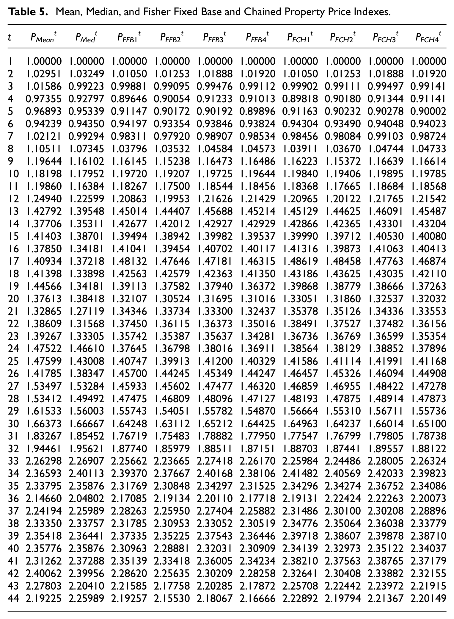
We conclude this section by forming aggregate residential property price indexes for Richmond. The price and quantity series for land and structures, P _Lk ^t , P _Sk ^t , Q _Lk ^t , Q _Sk ^t for k = 1, 2, 3, 4, are listed in Tables 3 and 4. The fixed base (FB) and chained (CH) Fisher (1922) ideal indexes for the four models, P _FFBk ^t and P _FCHk ^t for k = 1, 2, 3, 4, are listed in Table 5 along with simple mean and median property price indexes, P _Mean ^t and P _Med ^t .

Table 5.

Mean, Median, and Fisher Fixed Base and Chained Property Price Indexes.

t	P Mean t	P Med t	P FFB 1 t	P FFB 2 t	P FFB 3 t	P FFB 4 t	P FCH 1 t	P FCH 2 t	P FCH 3 t	P FCH 4 t
1	1.00000	1.00000	1.00000	1.00000	1.00000	1.00000	1.00000	1.00000	1.00000	1.00000
2	1.02951	1.03249	1.01050	1.01253	1.01888	1.01920	1.01050	1.01253	1.01888	1.01920
3	1.01586	0.99223	0.99881	0.99095	0.99476	0.99112	0.99902	0.99111	0.99497	0.99141
4	0.97355	0.92797	0.89646	0.90054	0.91233	0.91013	0.89818	0.90180	0.91344	0.91141
5	0.96893	0.95339	0.91147	0.90172	0.90192	0.89896	0.91163	0.90232	0.90278	0.90002
6	0.94239	0.94350	0.94197	0.93354	0.93846	0.93824	0.94304	0.93490	0.94048	0.94023
7	1.02121	0.99294	0.98311	0.97920	0.98907	0.98534	0.98456	0.98084	0.99103	0.98724
8	1.10511	1.07345	1.03796	1.03532	1.04584	1.04573	1.03911	1.03670	1.04744	1.04733
9	1.19644	1.16102	1.16145	1.15238	1.16473	1.16486	1.16223	1.15372	1.16639	1.16614
10	1.18198	1.17952	1.19720	1.19207	1.19725	1.19644	1.19840	1.19406	1.19895	1.19785
11	1.19860	1.16384	1.18267	1.17500	1.18544	1.18456	1.18368	1.17665	1.18684	1.18568
12	1.24940	1.22599	1.20863	1.19953	1.21626	1.21429	1.20965	1.20122	1.21765	1.21542
13	1.42792	1.39548	1.45014	1.44407	1.45688	1.45214	1.45129	1.44625	1.46091	1.45487
14	1.37706	1.35311	1.42677	1.42012	1.42927	1.42929	1.42866	1.42365	1.43301	1.43204
15	1.41403	1.38701	1.39494	1.38942	1.39982	1.39537	1.39990	1.39712	1.40530	1.40080
16	1.37850	1.34181	1.41041	1.39454	1.40702	1.40117	1.41316	1.39873	1.41063	1.40413
17	1.40934	1.37218	1.48132	1.47646	1.47181	1.46315	1.48619	1.48458	1.47763	1.46874
18	1.41398	1.33898	1.42563	1.42579	1.42363	1.41350	1.43186	1.43625	1.43035	1.42110
19	1.44566	1.34181	1.39113	1.37582	1.37940	1.36372	1.39868	1.38779	1.38666	1.37263
20	1.37613	1.38418	1.32107	1.30524	1.31695	1.31016	1.33051	1.31860	1.32537	1.32032
21	1.32865	1.27119	1.34346	1.33734	1.33300	1.32437	1.35378	1.35126	1.34336	1.33553
22	1.38609	1.31568	1.37450	1.36115	1.36373	1.35016	1.38491	1.37527	1.37482	1.36156
23	1.39267	1.33305	1.35742	1.35387	1.35637	1.34281	1.36736	1.36769	1.36599	1.35354
24	1.47522	1.46610	1.37645	1.36798	1.38016	1.36911	1.38564	1.38129	1.38852	1.37896
25	1.47599	1.43008	1.40747	1.39913	1.41200	1.40329	1.41586	1.41114	1.41991	1.41168
26	1.41785	1.38347	1.45700	1.44245	1.45349	1.44247	1.46457	1.45326	1.46094	1.44908
27	1.53497	1.53284	1.45933	1.45602	1.47477	1.46320	1.46859	1.46955	1.48422	1.47278
28	1.53412	1.49492	1.47475	1.46809	1.48096	1.47127	1.48193	1.47875	1.48914	1.47873
29	1.61533	1.56003	1.55743	1.54051	1.55782	1.54870	1.56664	1.55310	1.56711	1.55736
30	1.66373	1.66667	1.64248	1.63112	1.65212	1.64425	1.64963	1.64237	1.66014	1.65100
31	1.83267	1.85452	1.76719	1.75483	1.78882	1.77950	1.77547	1.76799	1.79805	1.78738
32	1.94461	1.95621	1.87740	1.85979	1.88511	1.87151	1.88703	1.87441	1.89557	1.88122
33	2.26298	2.26907	2.25662	2.23665	2.27418	2.26170	2.25984	2.24486	2.28005	2.26324
34	2.36593	2.40113	2.39370	2.37667	2.40168	2.38106	2.41482	2.40569	2.42033	2.39823
35	2.33795	2.35876	2.31769	2.30848	2.34297	2.31525	2.34296	2.34274	2.36752	2.34086
36	2.14660	2.04802	2.17085	2.19134	2.20110	2.17718	2.19131	2.22424	2.22263	2.20073
37	2.24194	2.25989	2.28263	2.25950	2.27404	2.25882	2.31486	2.30100	2.30208	2.28896
38	2.33350	2.33757	2.31785	2.30953	2.33052	2.30519	2.34776	2.35064	2.36038	2.33779
39	2.35418	2.36441	2.37335	2.35225	2.37543	2.36446	2.39718	2.38607	2.39878	2.38710
40	2.35776	2.35876	2.30963	2.28881	2.32031	2.30909	2.34139	2.32973	2.35122	2.34037
41	2.31262	2.37288	2.35139	2.33418	2.36005	2.34234	2.38210	2.37563	2.38765	2.37179
42	2.40062	2.39956	2.28620	2.25635	2.30209	2.28258	2.32641	2.30408	2.33882	2.32155
43	2.27803	2.20410	2.21585	2.17758	2.20285	2.17872	2.25708	2.22442	2.23972	2.21915
44	2.19225	2.25989	2.19257	2.15530	2.18067	2.16666	2.22892	2.19794	2.21367	2.20149

The above indexes are plotted in Figure 3.

Figure 3.

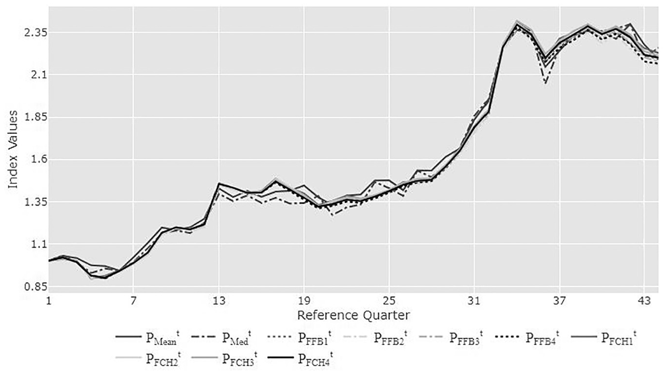
Mean, median, and Model 1 to 4 fixed base and chained fisher property price indexes.

It can be seen that the Mean and Median price index series, P _Mean ^t and P _Med ^t , are more volatile than the Fisher indexes which are very close to each other. However, P _Mean ^t and P _Med ^t do capture the trends in Richmond property prices over the sample period. The Model 4 fixed base and chained Fisher indexes differ by 1.6% for the final quarter in our sample so chain drift is not a major problem with the Model 4 aggregate property price indexes.

Our conclusion here is that it appears that Model 1, which has only a single geometric depreciation rate and uses information on land plot size, structure size, and the age of the structure, generates an aggregate property price index which approximates our subsequent hedonic regression Models which require additional information on housing characteristics. However, in order to obtain more accurate depreciation rates and to obtain more accurate subindexes for the land and structure components, additional information on property characteristics is required. Information on property location, the floor space area of the structure, the land plot area, and the age of the structure can be sufficient to generate land and structure price indexes that are reasonably accurate, provided that the fit of the hedonic regression is reasonably high.

Of course, additional information on the characteristics of the properties will in general improve the fit of the model. We used the number of bathrooms and bedrooms as indicators of structure quality because these structure characteristics were readily available. But many additional characteristics of the structure could be used as quality adjusting characteristics such as the type of construction, the “greenness” of the structure, the footprint of the structure, and so on. Also, there are characteristics which affect the quality of the land component of property value, such as distance to the nearest bus stop or subway station, distance to schools and hospitals, landscaping and possible views. An alternative to using postal codes as quality adjustment factors for land is the use of spatial coordinates; see for example, Diewert and Shimizu (2022). Moreover aspects of the theoretical model could be improved; the treatment of depreciation could be generalized and alternative smoothing methods could be used to smooth the structure price levels.

It is often difficult to obtain an estimate for the age of a structure and the following question was raised: What happens to Model 4 if we omit the Age variable? Thus, we ran the Model 4 regression without the age variable and the log likelihood fell from 2,771.88 to 1,060.3398. The R² between the observed and predicted variable fell from .8732 to .8380. The Land, Structure, and overall Property Price indexes that resulted when we dropped the Age variable captured the observed trends in the Model 4 indexes but had a considerable amount of bias. At the end of the sample period, the ratio of the new Land Price index to the Model 4 index was 2.167/2.464 = 0.879, the ratio of the new Structure Price index to the Model 4 index was 1.960/1.744 = 1.124, and the ratio of the new overall Chained Fisher Property Price index to the Model 4 Chained Fisher Property Price index was 2.089/2.201 = 0.949. Thus, it seems to be important to include the Age variable in resale property price hedonic regressions in order to avoid bias.

The above regressions used the data for the entire sample period. In the following section, we address the problems associated with the production of a real time index.

5. The Construction of Real Time Price Indexes

The period t price and quantity levels for land and structures that were constructed in the previous section were constructed for a window of forty-four quarters. How exactly should the quarter 45 indexes be constructed when the data for quarter 45 becomes available? More generally, how should real time land and structure price levels and indexes be constructed? We address these questions in this section.

We introduce some notation so that we can explain alternative price updating methods more precisely. Let P ^t be a period t price level that is derived from a hedonic regression for t = 1, 2, …, T. Our Models 1 to 4 generate two sets of price levels: one for constant quality land and another for constant quality structures. Think of the P ^t as representing one of these series for one of our hedonic regression models and let Q ^t be the companion period t quantity level. The product of P ^t and Q ^t is the value V ^t . We would like our price levels to satisfy the following transitivity relations:

$$P^t/P^r=\left(P^t/P^s\right)\left(P^s/P^r\right);1\le r\le s\le T.$$

(25)

Of course, if the P ^t satisfy the equalities in (25) and V ^t  = P ^t Q ^t for t = 1, …, T, then the Q ^t will also satisfy the transitivity conditions Q ^t /Q ^r  = (Q ^t /Q ^s )(Q ^s /Q ^r ) for 1 ≤ r < s < t ≤ T.

The above relations Equation (25) are equivalent to Fisher’s (1922, 270) Circularity Test for bilateral index number formulae. If the estimated price levels from a hedonic regression satisfy Equation (25), then the resulting price index will not have a chain drift problem which can be a serious problem as was discussed in Section 1.

In order to generate a real time sequence of price levels, run a hedonic regression that uses only the data for periods 1 and 2. Denote the resulting period 1 and 2 price levels for regression 1 as P¹(1) and P²(1). Define the real time price levels to be P^1*≡P¹(1) and P^2*≡P²(1). When the data for period 3 becomes available, run a second regression using only the data for periods 2 and 3. This second regression generates period 2 and 3 price levels, P²(2) and P³(2). Define the real time period 3 price level as P^3*≡P^2*[P³(2)/P²(2)]. Thus we update the period 2 real time price level P^2* by the price ratio or movement P³(2)/P²(2) in the price levels generated by our second hedonic regression that used only the data for periods 2 and 3. The third bilateral hedonic regression uses only the data for periods 3 and 4 and the real time price level for period 4 is defined as P^4*≡P^3*[P⁴(3)/P³(3)]. This updating process is continued indefinitely. This updating method is known as movement splicing, and it can be traced back to Court (1939, 109–11). The problem with this methodology is that the resulting price levels are not transitive, that is, they do not satisfy the restrictions Equation (25) and hence may be subject to chain drift.

Next, we consider a generalization of the above time dummy, adjacent period approach to the production of real time price levels. Instead of choosing to update the previous real time price levels by using bilateral hedonic regressions which use only the data for two adjacent periods, we use the data for M consecutive periods. First, choose M to be large enough so that the M period hedonic regression model will yield “reasonable” results; this will be the window length for the sequence of regression models that will be estimated. Second, run an initial regression model using the data for the first M periods and calculate the price levels pertaining to the first M periods in the data set. Next, a second regression model is estimated where the data consist of the initial data less the data for period 1 but adding the data for period M + 1. Appropriate price levels are calculated for this new regression model but only the rate of increase of the price level going from period M to M + 1 is used to update the previous sequence of M index values. This procedure is continued with each successive regression dropping the data of the previous earliest period and adding the data for the next period, with one new update factor being added with each regression. If the window length is a year, then this procedure is called a rolling year hedonic regression model and for a general window length, it is called a rolling window hedonic regression model with a movement splice. This is exactly the procedure used by Shimizu, Nishimura, and Watanabe (2010) and Shimizu, Takatsuji, et al. (2010) in their hedonic regression models for Tokyo house prices.

It turns out that there are several ways for linking the results of a new hedonic regression that uses a window length equal to M periods to the results of a previous rolling window regression. Let the price levels generated by the first regression be denoted by P¹(1), P²(1), …, P ^M (1) and set the “real time” sequence of price levels for the first M periods, P ^t* , to equal the corresponding P ^t (1), that is, we have P ^t* ≡P ^t (1) for t = 1, 2, …, M. The second regression drops the period 1 data and adds the period M + 1 data and generates the price levels P²(2), P³(2), …, P^M+1(2). Using the movement splice, the “real time” price level for period M + 1 is defined as P^M+1*≡P^M*[P^M+1(2)/P ^M (2)]. Using what is called a “window splice,” the “real time” price level for period M + 1 is defined as P^M+1*≡P^2* [P^M+1(2)/P²(2)]. The third regression drops the period 1 and 2 data and adds the period M + 1 and M + 2 data and generates the price levels P³(3), P⁴(3), …, P^M+2(3). Using the movement splice, the “real time” price level for period M + 2 is defined as P^M+2*≡P^M+1*[P^M+2(3)/P^M+1(3)]. Using the window splice, the “real time” price level for period M + 2 is defined as P^M+2*≡P^3*[P^M+2(3)/P³(3)].

The term and the concept of a window splice is due to Krsinich (2016). She recommended the use of window splicing over movement splicing because the time dummy variables in a rolling window hedonic regression are determined more accurately for the time dummy coefficients at the beginning of the window relative to the time dummy coefficients at the end of the window.

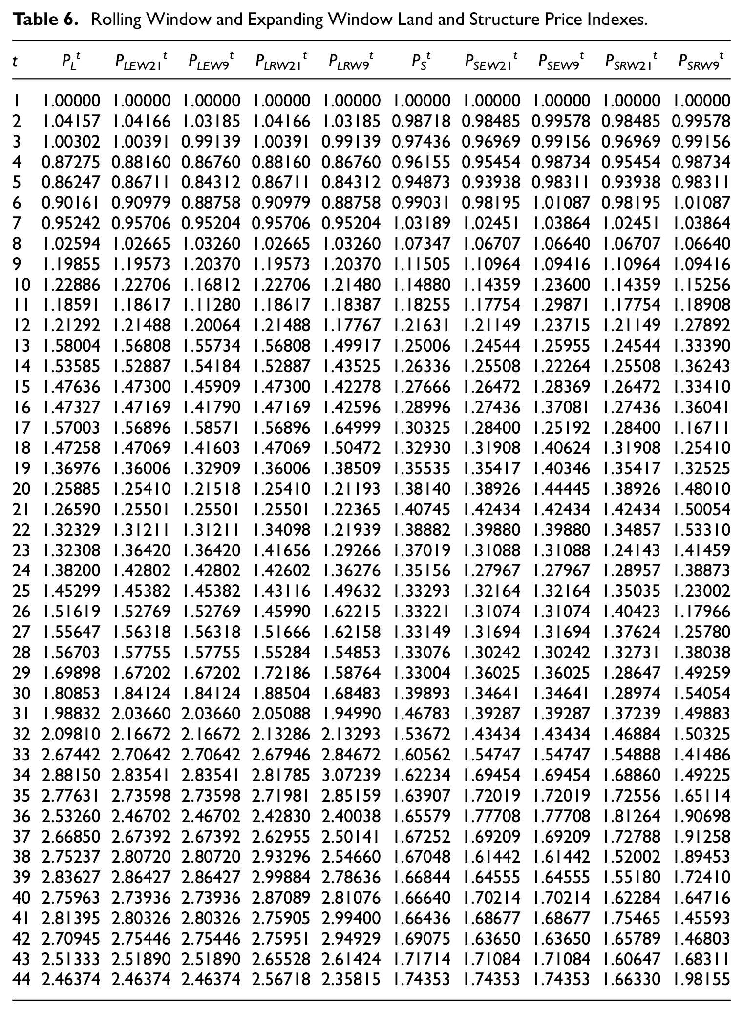
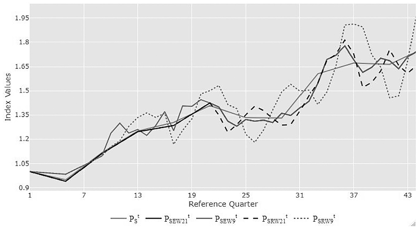
We calculated Rolling Window real time price levels for our data using Model 4 for window lengths M equal to 9 (which uses two years of data in the window) and 21 quarters (which uses five years of data) and using window splices to update the previous real time price levels. Denote these land price levels for quarter t as P _{LRW 9} ^t and P _{LRW 21} ^t and the corresponding structure price levels for quarter t as P _{SRW 9} ^t and P _{SRW 21} ^t for t = 1, …, 44. The various price levels were normalized to equal 1 in quarter 1. These (normalized) series are listed in Table 6. For comparison purposes, the Model 4 (normalized) land price levels P _{L 4} ^t and (normalized) structure price levels P _{S 4} ^t that are listed in Table 3 are also listed in Table 6 as P _L ^t and P _S ^t .

Table 6.

Rolling Window and Expanding Window Land and Structure Price Indexes.

t	P L t	P LEW 21 t	P LEW 9 t	P LRW 21 t	P LRW 9 t	P S t	P SEW 21 t	P SEW 9 t	P SRW 21 t	P SRW 9 t
1	1.00000	1.00000	1.00000	1.00000	1.00000	1.00000	1.00000	1.00000	1.00000	1.00000
2	1.04157	1.04166	1.03185	1.04166	1.03185	0.98718	0.98485	0.99578	0.98485	0.99578
3	1.00302	1.00391	0.99139	1.00391	0.99139	0.97436	0.96969	0.99156	0.96969	0.99156
4	0.87275	0.88160	0.86760	0.88160	0.86760	0.96155	0.95454	0.98734	0.95454	0.98734
5	0.86247	0.86711	0.84312	0.86711	0.84312	0.94873	0.93938	0.98311	0.93938	0.98311
6	0.90161	0.90979	0.88758	0.90979	0.88758	0.99031	0.98195	1.01087	0.98195	1.01087
7	0.95242	0.95706	0.95204	0.95706	0.95204	1.03189	1.02451	1.03864	1.02451	1.03864
8	1.02594	1.02665	1.03260	1.02665	1.03260	1.07347	1.06707	1.06640	1.06707	1.06640
9	1.19855	1.19573	1.20370	1.19573	1.20370	1.11505	1.10964	1.09416	1.10964	1.09416
10	1.22886	1.22706	1.16812	1.22706	1.21480	1.14880	1.14359	1.23600	1.14359	1.15256
11	1.18591	1.18617	1.11280	1.18617	1.18387	1.18255	1.17754	1.29871	1.17754	1.18908
12	1.21292	1.21488	1.20064	1.21488	1.17767	1.21631	1.21149	1.23715	1.21149	1.27892
13	1.58004	1.56808	1.55734	1.56808	1.49917	1.25006	1.24544	1.25955	1.24544	1.33390
14	1.53585	1.52887	1.54184	1.52887	1.43525	1.26336	1.25508	1.22264	1.25508	1.36243
15	1.47636	1.47300	1.45909	1.47300	1.42278	1.27666	1.26472	1.28369	1.26472	1.33410
16	1.47327	1.47169	1.41790	1.47169	1.42596	1.28996	1.27436	1.37081	1.27436	1.36041
17	1.57003	1.56896	1.58571	1.56896	1.64999	1.30325	1.28400	1.25192	1.28400	1.16711
18	1.47258	1.47069	1.41603	1.47069	1.50472	1.32930	1.31908	1.40624	1.31908	1.25410
19	1.36976	1.36006	1.32909	1.36006	1.38509	1.35535	1.35417	1.40346	1.35417	1.32525
20	1.25885	1.25410	1.21518	1.25410	1.21193	1.38140	1.38926	1.44445	1.38926	1.48010
21	1.26590	1.25501	1.25501	1.25501	1.22365	1.40745	1.42434	1.42434	1.42434	1.50054
22	1.32329	1.31211	1.31211	1.34098	1.21939	1.38882	1.39880	1.39880	1.34857	1.53310
23	1.32308	1.36420	1.36420	1.41656	1.29266	1.37019	1.31088	1.31088	1.24143	1.41459
24	1.38200	1.42802	1.42802	1.42602	1.36276	1.35156	1.27967	1.27967	1.28957	1.38873
25	1.45299	1.45382	1.45382	1.43116	1.49632	1.33293	1.32164	1.32164	1.35035	1.23002
26	1.51619	1.52769	1.52769	1.45990	1.62215	1.33221	1.31074	1.31074	1.40423	1.17966
27	1.55647	1.56318	1.56318	1.51666	1.62158	1.33149	1.31694	1.31694	1.37624	1.25780
28	1.56703	1.57755	1.57755	1.55284	1.54853	1.33076	1.30242	1.30242	1.32731	1.38038
29	1.69898	1.67202	1.67202	1.72186	1.58764	1.33004	1.36025	1.36025	1.28647	1.49259
30	1.80853	1.84124	1.84124	1.88504	1.68483	1.39893	1.34641	1.34641	1.28974	1.54054
31	1.98832	2.03660	2.03660	2.05088	1.94990	1.46783	1.39287	1.39287	1.37239	1.49883
32	2.09810	2.16672	2.16672	2.13286	2.13293	1.53672	1.43434	1.43434	1.46884	1.50325
33	2.67442	2.70642	2.70642	2.67946	2.84672	1.60562	1.54747	1.54747	1.54888	1.41486
34	2.88150	2.83541	2.83541	2.81785	3.07239	1.62234	1.69454	1.69454	1.68860	1.49225
35	2.77631	2.73598	2.73598	2.71981	2.85159	1.63907	1.72019	1.72019	1.72556	1.65114
36	2.53260	2.46702	2.46702	2.42830	2.40038	1.65579	1.77708	1.77708	1.81264	1.90698
37	2.66850	2.67392	2.67392	2.62955	2.50141	1.67252	1.69209	1.69209	1.72788	1.91258
38	2.75237	2.80720	2.80720	2.93296	2.54660	1.67048	1.61442	1.61442	1.52002	1.89453
39	2.83627	2.86427	2.86427	2.99884	2.78636	1.66844	1.64555	1.64555	1.55180	1.72410
40	2.75963	2.73936	2.73936	2.87089	2.81076	1.66640	1.70214	1.70214	1.62284	1.64716
41	2.81395	2.80326	2.80326	2.75905	2.99400	1.66436	1.68677	1.68677	1.75465	1.45593
42	2.70945	2.75446	2.75446	2.75951	2.94929	1.69075	1.63650	1.63650	1.65789	1.46803
43	2.51333	2.51890	2.51890	2.65528	2.61424	1.71714	1.71084	1.71084	1.60647	1.68311
44	2.46374	2.46374	2.46374	2.56718	2.35815	1.74353	1.74353	1.74353	1.66330	1.98155

Rather than using a Rolling Window (RW) approach to the construction of real time indexes, it is possible to use an Expanding Window (EW) approach. It is necessary to choose a window length M to start the EW indexes. The first M observations in our sample of T periods act as “training” periods. Let the price levels generated by the first regression be denoted by P¹(1), P²(1), …, P ^M (1) and set the “real time” sequence of price levels for the first M periods, P ^t* , to equal the corresponding P ^t (1), that is, we have P ^t* ≡P ^t (1) for t = 1, 2, …, M. Thus, the real time price levels for the first M periods using the EW approach are the same as the corresponding RW price levels. Note that these price levels satisfy the transitivity conditions Equation (25) so there is no chain drift problem with these price levels. However, let us assume that the previous price levels P^1*, P^2*, …, P^M* cannot be revised. We use the window method for price updating the real time price levels. Thus, the EW “real time” price level for period M + 1 is defined as P^M+1*≡P^1*[P^M+1(2)/P¹(2)]. The third regression adds the period M + 1 and M + 2 data to the initial data set and generates the price levels P¹(3), P²(3), …, P^M+2(3). Using the window splice, the “real time” price level for period M + 2 is defined as P^M+2*≡P^1*[P^M+2(3)/P¹(3)]. The process continues in the same manner until the period T data has been added to the regression. The final Nonrevisable Expanding Window series does not satisfy the transitivity conditions Equation (25) but the final price level P^T* for the EW series cannot be unrealistically too high or too low because P^T* is the final price level for a sequence of price levels that does satisfy the transitivity conditions Equation (25).

In our particular context, it can be seen that the Expanding Window approach to linking in the results of a new regression with the results of previous regressions gives the same estimates as the Rolling Window approach for the first M periods. Other methods for linking the results of a new rolling window regression to previous index levels are the half splice due to de Haan (2015) and the mean splice suggested by Ivancic et al. (2011) and Diewert and Fox (2022).

Chessa (2016, 2021) introduced the concept of using an expanding window in a multilateral index number context. The idea of using an infinitely expanding window of observations arose in Diewert (2023) in his discussion of the multilateral index Predicted Share Method that used dissimilarity measures to link the current period price levels to past period price levels. The expanding window approach was used by Diewert and Shimizu (2023) in their analysis of laptop prices in Japan. Diewert (2024) discussed adapting this approach to other multilateral methods based on the use of econometrics. Note that the “real time” nature of the EW and RW approaches starts at period M, that is, at the end of the training periods.

There are at least two potential problems with the Expanding Window price levels:

• The EW sequence of real time price levels P ^t* could differ substantially from the sequence of price levels generated by the final hedonic regression P ^t (T−M + 1) for some t < T.

• The Expanding Window sequence of hedonic regressions does not allow for gradual changes in the underlying utility functions u(L) for land and U(S) for structures whereas the Rolling Window sequence of hedonic regressions does allow for changes in preferences.

Problem 1 can be addressed by comparing the real time EW price levels with the price levels generated by the final hedonic regression that uses the data for all T periods. If the discrepancies between the two series are not too large, then the EW price levels could be accepted as being reasonable.

Problem 2 can be addressed by looking at the fits of the various regressions that are used to calculate the EW price levels. If the fits are low, then other multilateral methods should be considered.

We calculated Expanding Window real time price levels for our data using Model 4 for window lengths M equal to 9 and 21 quarters and using window splices to update the previous real time price levels. Denote the resulting land price levels for quarter t as P _{LEW 9} ^t and P _{LEW 21} ^t and the corresponding structure price levels for quarter t as P _{SEW 9} ^t and P _{SEW 21} ^t for t = 1, …, 44. These (normalized) series are listed in Table 6 below.

Here are some points to notice about the above indexes:

• The Rolling Window and Expanding Window indexes for both land and structures that used the same number of periods as training periods (9 and 21 quarters) are equal for the training period quarters.

• The two Expanding Window indexes for land are equal to each other for quarters 22 to 44 and similarly for the two EW structure indexes.

• The two EW indexes for land, P _{LEW 9} ^t and P _{LEW 21} ^t , are equal to the Model 4 land index P _L ^t for t = 44. Similarly, P _{SEW 9}⁴⁴ and P _{SEW 21}⁴⁴ are equal to the Model 4 structure index P _S ⁴⁴.

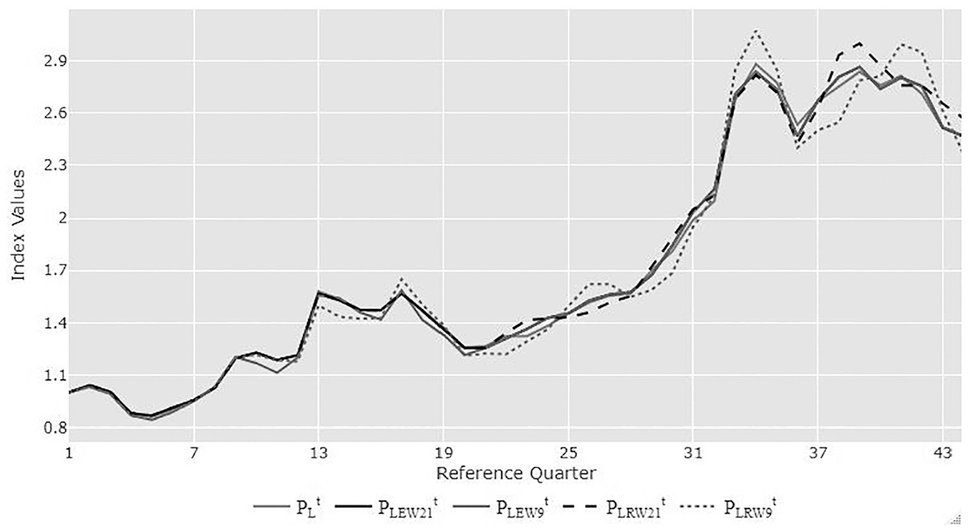
Figure 4 and Figure 5 plot the alternative Expanding Window and Rolling Window (normalized) price levels for Land and for Structures. The Model 4 indexes for Land are plotted as P _L ^t on Figure 4 and the Model 4 indexes for Structures are plotted as P _S ^t on Figure 5.

Figure 4.

Alternative rolling window and expanding window land price indexes.

Figure 5.

Alternative rolling window and expanding window structure price indexes.

The two Expanding Window series, P _{LEW 9} ^t and P _{LEW 21} ^t can barely be distinguished from the transitive Model 4 land price series, P _L ^t . Thus, the two real time EW land price series do not suffer from a major chain drift problem. The 21 quarter Rolling Window land price series, P _{LRW 21} ^t , is more volatile than the EW series and the 9 quarter Rolling Window land price series, P _{LRW 9} ^t , is even more volatile. However, the two RW series do capture the trends in Land prices.

Figure 5 shows that the real time Expanded Window structure price indexes that use the 9 and 21 quarter training periods, P _{SEW 9} ^t and P _{SEW 21} ^t , cannot be distinguished from each other. However, these Expanding Window structure indexes are much more volatile than the Model 4 structure price index P _S ^t that used the data for all forty-four quarters and is free from chain drift. This is an indication that the training period should be longer than twenty-one quarters in order to obtain less volatile indexes that are closer to being transitive. The Rolling Window structure price index that used 21 quarters of training data, P _{SRW 21} ^t , shows a great deal of volatility around P _S ^t and the index that used only 9 quarters of training data, P _{SRW 9} ^t , is even more volatile. However, all 4 EW and RW indexes do capture the trends in structure prices that are defined by P _S ^t  = P _{S 4} ^t .

To know how a Rolling Window approach using a mean splice would work for our data we computed land, structure, and overall Mean Splice indexes using a Rolling Window consisting of twenty-one quarters. The resulting Mean Splice Rolling Window land and structure indexes using a twenty-one-quarter training period were almost identical to the corresponding Expanding Window indexes using a twenty-one-quarter training period. Thus, we have not included these Mean Splice indexes in the above Figures. In a recent comprehensive simulation, von Auer (2025) showed that half splice and mean splice seemed to produce more reliable results than window splice and movement splice so there is room for additional research to determine the “best” way for linking the results of a new set of indexes with an existing set of indexes.

The overall conclusion that emerges from these figures is that the Expanded Window and Rolling Window with Mean Splice indexes based on the Model 4 specification of land and structure utility functions that use five years of training data led to relatively smooth land and structure subindexes that were largely free from chain drift. However, choosing a longer training period would probably improve the smoothness and transitivity of the resulting EW and RW indexes.

Finally, the price levels for land and structures that were generated by the five alternative sets of estimates presented in Table 6 can be combined with the Model 4 utility functions to generate aggregate property price indexes as was done in the previous section. Using chained Fisher indexes to aggregate over the structures and land indexes listed on Table 6 leads to Table 5 alternative aggregate property price indexes. The aggregate Fisher property price index that corresponds to the Model 4 aggregate prices, P _L ^t and P _S ^t listed in Table 6, is equal to the chained Fisher property price index P _{FCH 4} ^t that is listed in Table 5. Instead of using P _L ^t and P _S ^t listed in Table 6, we could use P _{LEW 21} ^t and P _{SEW 21} ^t and construct an alternative chained Fisher property price index. It turns out that this alternative property price index cannot be distinguished from P _{FCH 4} ^t that is listed in Table 5. Using the remaining three pairs of price indexes for land and structures that are listed in Table 6 led to alternative aggregate chained Fisher property price indexes that also could not be distinguished from P _{FCH 4} ^t . Thus, the various methods that were used to extend the aggregate property price index in real time, in the end, led to more or less the same aggregate property index.

In the following section, we use our data to construct “traditional” log price time dummy hedonic regressions and compare the resulting “traditional” indexes to the indexes generated by our additive approach to the property decomposition problem.

6. Estimating Structure Depreciation Rates from Traditional Log Price Hedonic Regression Models

A way of rationalizing the traditional log price time dummy hedonic regression model for properties with varying amounts of land area L and constant quality structure area S* is that the utility that these properties yield to purchasers is proportional to the Cobb-Douglas utility function L^αS^*β where α and β are positive parameters (which do not necessarily sum to one). The early analysis in this section follows that of McMillen (2003, 289–90) and Shimizu, Nishimura, and Watanabe (2010, 795). McMillen assumed that α + β = 1. We follow Shimizu, Nishimura, and Watanabe (2010) in allowing α and β to be unrestricted. Our depreciation model is somewhat different from the models of these authors. Initially, we assume that the constant quality structure area S* is equal to the floor space area of the structure, S, times an age adjustment, (1−δ) ^A , where A is the age of the structure in years and δ is a positive depreciation rate that is less than 1. Thus S* is related to S as follows:

$$S^{*}\equiv S(1-\delta {)}^A.$$

(26)

In any given time period t, we assume that the nominal value of a property, V _t , with the amount of land L and the amount of quality adjusted structure S* is equal to the following expression:

$$\begin{array}{c}\multicolumn{1}{c}{V_t=p_t{L}^{\alpha }{S}^{*\beta }}\\ \multicolumn{1}{c}{=p_t{L}^{\alpha }{\left[S{(1-\delta )}^A\right]}^{\beta }\mathrm{using}(26)}\\ \multicolumn{1}{c}{=p_t{L}^{\alpha }{S}^{\beta }(1-\delta {)}^{\beta A}}\\ \multicolumn{1}{c}{=p_t{L}^{\alpha }{S}^{\beta }{\varphi }^A}\end{array}$$

(27)

where p _t can be interpreted as a period t property price index and the constant ϕ is defined as follows:

$$\varphi \equiv (1-\delta {)}^{\beta }.$$

(28)

If we deflate V _t by the period t property price index p _t , we obtain the real value or utility u _t of the property with characteristics L and S*; that is, we have:

$$V_t/p_t=L^{\alpha }{S}^{*\beta }\equiv u_t.$$

(29)

Thus, u _t is the aggregate real value of the property with characteristics L and S*.

Define ρ _t as the logarithm of p _t and γ as the logarithm of ϕ, that is,

$${\rho }_t\equiv \ln P_t;\gamma \equiv \ln \varphi .$$

(30)

After taking logarithms of both sides of the last equation in Equation (27) and using definitions Equation (30), we obtain the following equation:

$$\ln V_t={\rho }_t+\alpha \ln L+\beta \ln S+\gamma A.$$

(31)

Log price hedonic regressions for property prices that are similar to Equation (31) date back to Bailey et al. (1963).

Suppose that we have N(t) sales of properties in a neighborhood in period t and the purchase price of property n is V _tn . Suppose that we have data for T periods. The characteristics associated with property n in period t are L _tn , S _tn , and A _tn . Assuming that the property purchaser valuation model defined by Equation (31) holds approximately, the logarithms of the period t property prices will satisfy the following equations:

$$\ln V_{\mathrm{tn}}={\rho }_t+\alpha \ln L_{\mathrm{tn}}+\beta \ln S_{\mathrm{tn}}+\gamma A_{\mathrm{tn}}+{\epsilon }_{\mathrm{tn}};t=1,\dots ,T;n=1,\dots ,N(t)$$

(32)

where the ε _tn are independently distributed error terms with 0 means and constant variances. It can be seen that (32) is a traditional log price time dummy hedonic regression model with a minimal number of characteristics. The unknown parameters in (32) are the constant quality log property prices, ρ₁, …, ρ _T , and the taste parameters α, β, and γ. Once these parameters have been determined, the geometric depreciation rate δ which appears in Equation (27) can be recovered from the regression parameter estimates as follows:

$$\delta =1-e^{\gamma /\beta }.$$

(33)

We now explain how the hedonic regression model defined by Equation (32) can be manipulated to provide a decomposition of property value in period t into land and quality adjusted structure components.

To justify the hedonic regression Equation (32), we assume that there is a period t constant quality price of property in period t equal to p _t (as before) and the period t value of a property with characteristics L and S* is given by the following period t property valuation function, V(p_t,L,S*), defined as follows:

$$V(p_t,L,S^{*})\equiv p_t{L}^{\alpha }{S}^{*\beta }=p_{t}u(L,S^{*})$$

(34)

where the purchaser cardinal utility function u is defined as u(L,S*) ≡L^αS^*β and α and β are positive parameters which parameterize the purchaser’s cardinal utility function. p _t is the period t constant quality price of a property with land and quality adjusted structures equal to L and S*≡S(1−δ) ^A . In our empirical work, our estimates for α and β are such that α + β is always substantially less than 1. This means that a property in a given period that has double the land and quality adjusted structure than another property will sell for less than double the price of the smaller property. This follows from the fact that our Cobb-Douglas utility function, u(L,S*) ≡L^αS^*β, exhibits diminishing returns to scale when α + β < 1; that is, we have:

$$u(\lambda L,\lambda S^{*})={\lambda }^{\alpha +\beta }u(L,S^{*})$$

(35)

for all λ > 0 where α + β < 1. This behavior is roughly consistent with our Models 3 and 4 where there was a tendency for property prices to increase less than proportionally as L and S* increased.

The marginal prices of land and constant quality structure in period t for a property with characteristics L and S*, π _tL (p_t,L,S*) and π _tS* (p_t,L,S*), are defined by partially differentiating the property valuation function with respect to L and S* respectively:

$${\pi }_{\mathrm{tL}}(p_t,L,S^{*})\equiv \partial V(p_t,L,S^{*})/\partial L\equiv p_t\alpha L^{\alpha }{S}^{*\beta }/L=\alpha V(p_t,L,S^{*})/L$$

(36)

$${\pi }_{t{S}^{*}}(p_t,L,S^{*})\equiv \partial V(p_t,L,S^{*})/\partial S^{*}\equiv p_t\beta L^{\alpha }{S}^{*\beta }/S^{*}=\beta V(p_t,L,S^{*})/S^{*}.$$

(37)

If we multiply the marginal price of land by the amount of land in the property and add to this value of land the product of the marginal price of constant quality structure by the amount of constant quality structure on the property, we obtain the following identity:

$$(\alpha +\beta )V(p_t,L,S^{*})={\pi }_{\mathrm{tL}}(p_t,L,S^{*})L+{\pi }_{t{S}^{*}}(p_t,L,S^{*})S^{*}.$$

(38)

If α + β is less than one, then using marginal prices to value the land and constant quality structure in a property will lead to a property valuation that is less than its selling price. Thus to make the land and structure components of property value add up to property value, we divide the marginal prices defined by Equations (36) and (37) by α + β in order to obtain the following adjusted constant quality prices of land and structures in period t, p_tL(p_t,L,S*) and p _tS* (p_t,L,S*):

$$p_{\mathrm{tL}}(p_t,L,S^{*})\equiv {\pi }_{\mathrm{tL}}(p_t,L,S^{*})/(\alpha +\beta )=\alpha {(\alpha +\beta )}^{-1}V(p_t,L,S^{*})/L;$$

(39)

$$p_{t{S}^{*}}(p_t,L,S^{*})\equiv {\pi }_{t{S}^{*}}(p_t,L,S^{*})/(\alpha +\beta )=\beta {(\alpha +\beta )}^{-1}V(p_t,L,S^{*})/S^{*}.$$

(40)

The above material outlines a theoretical framework that could be used to generate a decomposition of property value into land and structure components using the results of a traditional log price time dummy hedonic regression model like Equation (32). Unfortunately, any such decomposition is not likely to be satisfactory. Consider a hypothetical property in periods t and t + 1 where the quantities of constant quality land L and constant quality structure S* remain constant and consider the growth of the price land and structure price levels for this hypothetical property defined by Equations (39) and (40). It can be seen that p _{t+ 1},_L/p_t, _L  = p _{t +1},_S*/p_t, _S*  = V(p _{t +1},L,S*)/V(p_t,L,S*); that is, constant quality price change for structures and for land going from period t to period t + 1 for a constant quality property is equal to the growth in property value going from period t to t + 1. This means that constant quality land and structure prices move in a proportional manner for constant quality properties. But in fact, we observe different rates of change in land and structure prices over time. Moreover, the Cobb-Douglas utility function assumption implies that the land and structure shares of a constant quality property remain constant over time. This is also unlikely to be true. Also, our additive decomposition of property value allows for properties with no structure whereas the Cobb-Douglas model breaks down if S _tn  = 0. However, these unrealistic aspects of the Cobb-Douglas utility model for residential properties does not mean that this framework cannot generate useful overall property price indexes (for properties with structures) as we will show below.

The hedonic regression model defined by Equation (32) can be generalized to the following model defined by Equation (41), which has added the location, bathroom and bedroom dummy variables, to Equation (32):

$$\begin{array}{c}\multicolumn{1}{c}{\ln V_{\mathrm{tn}}={\rho }_t+\alpha \ln L_{\mathrm{tn}}+\beta \ln S_{\mathrm{tn}}+\gamma A_{\mathrm{tn}}+\sum _{j=2}^6{\omega }_j{D}_{\mathrm{PC},\mathrm{tn},j}+}\\ \multicolumn{1}{c}{\sum _{j=2}^6{\eta }_j{D}_{\mathrm{BA},\mathrm{tn},j}+\sum _{j=4}^6{\theta }_j{D}_{\mathrm{BE},\mathrm{tn},j}+{\epsilon }_{\mathrm{tn}}}\\ \multicolumn{1}{c}{}\\ \multicolumn{1}{c}{t=1,\dots ,T;n=1,\dots ,N(t).}\end{array}$$

(41)

The postal code dummy variables, D _PC , _tn , _j were defined by Equation (4) for j = 1, …, 6; the bathroom dummy variables, D _BA , _tn,j , were defined for Equation (12) for j = 1, …, 6 and the bedroom dummy variables, D _BE , _tn,j , were defined for Equation (14) for j = 3, …, 6. To prevent exact multicollinearity in the hedonic regression defined by Equation (41), we set ω₁ = 0, η₁ = 0, and θ₃ = 0.

We used our Richmond data set and ran the hedonic regression defined by Equation (41). The R² for this regression turned out to be .8734 which is comparable to the R² we obtained for our Model 4 nonlinear regression. The estimated coefficients for α*, β*, and γ* were 0.39676, 0.25742, and −0.008062 respectively with T statistics equal to 60.64, 28.09, and −50.71. The corresponding annual structure geometric depreciation rate defined by Equation (32) was δ*≡ 1 −e^γ*/β* = 0.03084 or 3.084% per year. This is fairly close to the average of the estimated structure depreciation rates that were generated by Models 3 and 4 (3.28% and 2.81% per year).

The time dummy coefficients were used to generate the sequence of quarterly residential property price levels by exponentiating the estimated ρ _t *. Define the quarter t property price level, P _Prop ^t ≡exp(ρ _t *) for t = 1, …, 44. Construct the Hedonic Property Price Index for quarter t as P _HED ^t ≡P _Prop ^t /P_Prop¹ for t = 1, …, 44. The resulting Hedonic overall property price indexes P _HED ^t were very close to the Fisher Fixed Base and Chained property price indexes, P _{FFB 4} ^t and P _{FCH 4} ^t that were listed in Table 5. The partial correlations of P _HED ^t with P _{FFB 4} ^t and P _{FCH 4} ^t were .99943 and .99952 respectively. Thus, for our particular data set, the traditional log price time dummy hedonic regression model generated almost the same aggregate property price index as was generated by our Model 4 nonlinear hedonic regression. Figure 6 plots the two Fisher indexes along with the traditional hedonic property price index.

Figure 6.

Traditional hedonic model and purchaser’s model property price indexes.

7. Conclusion

Some of the tentative conclusions we can draw from the paper are as follows:

• Our consumer or purchaser approach to developing residential property price indexes that can generate sensible subindexes for the structure and land components of the property worked well for our particular data set. We solved the multicollinearity problem between structure and land size by smoothing (over time) the implied constant quality structure prices.

• Our purchaser approach provides an alternative to McMillen’s Cobb-Douglas preferences approach. Our approach is based on separate sub-utility functions for the land and structure components of residential property value. A problem with McMillen’s approach is that it implies that constant quality structure price movements are equal to constant quality land price movements. Another problem with Cobb-Douglas preferences is that this model cannot deal with properties that have no structure whereas our additive decomposition approach can deal with this situation.

• The information on property characteristics that we required in order to have a hedonic regression model that fits the data reasonably well was fairly modest. We required information on the purchase prices for the properties in scope, the structure floor space and land plot areas, the age of the structure and some information on the location of the property such as postal code information or spatial coordinate information. Some additional information on housing characteristics that can be used to characterize the quality of the structure is useful. For our Model 4, we used the number of bedrooms and the number of bathrooms as quality indicators. Other indicators will no doubt be useful.

• It is important to eliminate extreme outliers on both purchase prices and on the property characteristics. Isolated extreme observations at the tails of the distribution of prices and property characteristics lead to poorly determined hedonic surfaces.

• Introducing splines on the land plot area proved to be very important for our example.

• Simple mean and median property price indexes generated property price indexes that captured the trend in our constant quality property price indexes. However, these indexes are much more volatile than our hedonic property price indexes.

• The traditional log price time dummy variable hedonic regression approach generated overall property price indexes which were virtually identical to our purchaser model overall property price indexes when both types of models used more or less the same characteristics. This result is useful in the context of trying to use existing information on residential property price indexes along with information on the capital stock of residential structures in order to provide a complete decomposition of residential property value into land and structure subcomponents; see Davis and Heathcote (2007) for a useful methodology that accomplishes this task.

• The traditional log price time dummy hedonic regression approach generated an implied geometric structure depreciation rate which was close to our Model 3 and 4 depreciation rates. This is a very encouraging result.

• Finally, we considered the problems associated with producing real time indexes as opposed to producing retrospective indexes. We applied the Rolling Window and Expanding Window methodologies to this problem and found that for our particular data set, the Expanding Window approach generated smoother price indexes for the land and structure components of residential properties in Richmond. The Rolling Window approach with mean splicing with a window of twenty-one quarters produced results that were virtually the same as the Expanding Window approach.