
Abstract
In recent years, researchers and statisticians have increasingly used econometric techniques to generate timely, high-quality, and detailed official statistics. This study presents a modified form of regression-based temporal disaggregation model to compile the index of production in construction for Türkiye, employing a state-space modeling approach. The model incorporates the twelve-month moving sum of deflated turnover as an observed variable and the number of employees as an exogenous variable. Finally, four alternative models—three assuming constant labor productivity and one assuming time-varying labor productivity—are compared.
Keywords
1. Introduction
The general economy and construction industry maintain a close relation, as evidenced by the strong interconnections between the construction industry and other sectors. Spillover effects from developments in the construction industry stimulate various sectors within the economy. These developments generate significant demand for intermediate input from other sectors, such as agriculture, manufacturing, transportation, mining, and services. Notably, developments in other sectors that need capital facilities to produce goods and services also affect the construction industry (K’Akumu 2009). Given its predominant domesticity and labor-intensiveness, the construction industry serves as a significant source of employment opportunities in the economy. Therefore, the quality of construction statistics holds strategic importance for effective economic planning and decision-making. When National Statistical Institutes (NSIs) ensure the provision of more reliable, accurate, and timely statistics, decision-makers can respond appropriately and implement timely strategic policies to address economic fluctuations (Fan et al. 2011).
The index of production in construction (IPC) is a theoretical measure that aims to show changes in the volume of value-added data. However, as monthly value-added data are typically unavailable, NSIs use some proxy variables such as output quantities, building permits and starts, hours worked, employment, material input, wages and salaries, and turnover to estimate the IPC (Eurostat 2011). Until the end of 2016, a productivity-corrected hours worked method had been used to compile the IPC in Türkiye, primarily relying on the hours worked survey as the data source. However, in 2016, Turkstat decided to increase the weight of administrative data sources in the production of official statistics to reduce data compilation costs while alleviating the respondent burden. Consequently, Turkstat discontinued certain surveys, including the hours worked survey, and shifted to predominantly utilizing value-added tax (VAT) registers to generate short-term production statistics.
The IPC continuation with the variable of deflated turnover is one of the methods suggested by Eurostat (2011). This method relies on the assumption that monthly deflated turnover is an approximation for monthly gross production. However, just like other administrative data sources, tax records are not designed specifically for statistical purposes. A significant seasonal bias arises in the variable turnover obtained from the monthly VAT registers in Türkiye, as the usual practice for enterprises and corporations is to declare to the government for taxation and other accounting purposes at the end of the calendar year. Owing to inconsistencies between the timing of work done and timing of recording, the seasonal pattern of the deflated turnover does not reflect the actual seasonal pattern of the production in construction, indicating that the deflated turnover may not represent an appropriate proxy variable for value-added data in Türkiye.
Temporal disaggregation (TD) techniques exhibiting varying applications in the production of short-term official statistics could be a solution to the aforementioned problem. Temporal disaggregation could be defined as the process of deriving high-frequency time series from the low frequency series. Temporal disaggregation methods are broadly classified into two main categories based on the availability of high-frequency information regarding the target variable. The first group includes methods that do not use an indicator (Durbin and Quenneville 1997; Hillmer and Trabelsi 1987; Lisman and Sandee 1964; Stram and Wei 1986; Wei and Stram 1990). The second category comprises methods employing high-frequency information from related indicators, such as the Denton procedure (Denton 1971), regression-based methods (Chow and Lin 1971; Dagum and Cholette 2006; Fernández 1981; Litterman 1983), and dynamic regression models (Di Fonzo 2003; Proietti 2006; Silva and Cardoso 2001).
The issue of seasonal bias can be addressed through temporal disaggregation techniques such as employing an appropriate high-frequency indicator that captures the expected seasonal variations in construction production. However, standard temporal disaggregation methods can lead to too large revisions, especially in annual growth rates, as they require extrapolation in months beyond the temporal range for which low-frequency data are not yet available. Therefore, we propose a modified form of regression-based temporal disaggregation technique (MTD) to overcome both the seasonal bias problem and revision issue. The MTD mainly differs from the standard temporal disaggregation because we derive the monthly IPC from the monthly rolling annualized totals of the turnover series instead of the standard annual totals corresponding to each calendar year. The most important contribution of MTD is that it eliminates the need for extrapolation, as the most up-to-date information on annual turnover is used each month, which reduces revisions significantly compared to standard temporal disaggregation. However, as the model parameters are re-estimated every month, revisions still occur but are now quite small.
Because labor input is used for updating IPC, the regression coefficient can be considered as labor productivity. A crucial underlying assumption in standard regression-based temporal disaggregation models is the constancy of the relation between variables (low-frequency and high-frequency related data). However, this assumption may not work well when the relation varies with time or when structural breaks are present within the data. Empirical evidence indicates that dynamics between macroeconomic variables may change in the long run (Stock and Watson 1996). Keeping this economic reality in mind, MTD is extended to explicitly account for changes in labor productivity over time. We compare four alternative models, with three assuming constant labor productivity and one assuming time-varying labor productivity.
We use a state-space model (SSM) for estimation as it enables the estimation of unobserved latent variables, such as labor productivity, and allows the calculation of time-varying parameters, offering a more flexible and dynamic modeling approach. The SSM approach to temporal disaggregation was originally introduced by Harvey and Pierse (1984) and further developed by Durbin and Quenneville (1997) and Harvey and Koopman (1997). More recently, Moauro and Savio (2005) used SUTSE models for temporal disaggregation, and Proietti (2006) contributed to the field of regression-based temporal disaggregation within the SSM framework. Labonne and Weale (2020) employed the SSM framework to derive monthly business sector output from overlapping noisy quarterly UK VAT data, which has similarities to our problem. This study considers the changing nature of relations between variables in temporal disaggregation application. To our knowledge, this represents the first known use of time-varying coefficients as explanatory variables in this context.
The remainder of this paper is divided into six sections. Section 2 discusses the main data sources and variables for IPC compilation; Section 3 provides an overview of the general SSM and describes the proposed models for compiling Turkish IPC; Section 4 discusses the estimation results, Section 5 provides a general discussion of MTD, and finally, Section 6 provides concluding remarks.
2. Data Sources and Variables for IPC Compilation
Despite the strategic significance of the construction sector, the compilation of production statistics for this industry poses considerable challenges worldwide due to its inherent characteristics (Ruddock 2002). In general, construction activities are mainly project-based and are characterized by short-term temporary partnerships between different companies (Eurostat 2011). Although the duration of a particular project is limited, it generally lasts longer than the accounting period (United Nations 1997). A significant portion of enterprises in the construction sector are small firms. However, even in large firms, much of the work is often subcontracted (Meikle and Grilli 1999). The widespread practice of subcontracting in the formal and informal sectors introduces the probability of double counting or omissions. An important share of construction activity may be unrecorded or under-recorded. First, a considerable amount of construction work is done by establishments whose main activities are unclassified under the construction sector (United Nations 1997). Second, construction work is generally geographically dispersed, even for the same enterprise. Notably, maintaining a comprehensive register or database for collecting data from the construction sector is challenging due to the temporary nature of construction sites, which are often dispersed across numerous locations (Windapo and Qongqo 2011). In addition, numerous small-scale firms enter and exit from the industry in response to changing economic conditions each year (Briscoe 2006). Owing to the footloose nature of the industry, the operations of these firms may not be captured in construction statistics (Briscoe 2006; K’Akumu 2007).
Two national account concepts for defining construction activity include gross output and gross value-added. While the former is usually measured, the latter must always be estimated (Meikle and Grilli 1999). Gross output is the turnover of the construction sector or the amount paid for construction work by its final customers. Gross value-added is the value-added by the construction industry itself; hence, it should exclude inputs from other parts of the economy to avoid double counting (Meikle and Gruneberg 2015). In other words, gross output is a more general concept than gross value-added, as it includes the total value of all inputs in construction work in addition to gross value-added.
The IPC aims to measure the changes in volume of value-added data at close and regular intervals, normally monthly. As monthly value-added data are generally unavailable, NSIs employ some variables or combinations of variables to estimate the IPC to substitute value-added data. These variables are output quantities, building permits and starts, hours worked, material input, wages and salaries, turnover, and subcontracting (Eurostat 2011).
Best and Meikle (2015) emphasized that poor data will yield poor results, regardless of the employed method. Due to the idiosyncratic features of the construction industry, collecting reliable and timely construction data is always troublesome. The two main data sources of construction output statistics are administrative sources and surveys. Administrative sources are very useful for producing timely, detailed, and comprehensive statistics. Although administrative register-based data compilation offers advantages such as cost-effectiveness and reduced burden on respondents, data quality may be adversely affected by classification and coverage issues, outliers, data entry errors, and reporting delays of construction enterprises (Eurostat 2011). Surveys are subject to sampling, coverage, and distribution problems, but more importantly, they can be disadvantageous in terms of meeting the timeliness criteria of good quality statistics. Often, surveys are used where suitable administrative data are unavailable or insufficient to produce IPC.
Where monetary data (turnover, value of output, wages and salaries, or value of purchased materials) are collected, deflation is necessary, as the IPC is a volume measure. The selection of representative price indices for generating construction output at constant prices presents certain challenges. Output prices or purchaser prices are considered ideal deflators for methods based on turnover or output value. Since an output price index shows the development of final prices by the client to the contractor for completed construction work, it reflects both changes in productivity and profitability (Best and Meikle 2015). Similarly, with methods based on input values (wages and salaries, value of input material), input prices paid for labor, purchased material, and equipment by contractors should be used. If indices for input costs are used instead of output price indices to obtain IPC by deflating turnover or output value, the deflators will systematically overstate price changes and underestimate growth in output and productivity (Valence 1996). The reason is that marginal cost shocks do not fully pass through to final product prices at the firm level and final output prices do not reflect completely changes in costs (Klenow and Willis 2016).
Where quantity data (such as square meters of built area or cubic meters of volume) are collected, deflation is unnecessary. However, owing to the heterogeneity of construction output and quality differences even for buildings of the same size and type, quantity-based measurements would be misleading (Eurostat 2011).
When labor input (hours worked and number of persons employed) is used to update the IPC, labor productivity changes must be considered, suggesting that a productivity factor must be estimated. Common practice is to use the productivity trend observed in the past for the current reference period and to benchmark monthly IPC to quarterly series of construction value-added data. However, this may lead to large revisions in published monthly IPC if the relation between the quarterly series and hours worked is too noisy (Eurostat 2011). Because a single variable or data source is insufficient for compiling construction output statistics alone, some countries use combinations of variables or data sources to overcome the aforementioned problems.
2.1. Data Sources and Variables in Türkiye
The main data used in this study are the turnover and number of paid employees in construction industry obtained from Turkstat. Turnover statistics are based on VAT registers obtained from the Revenue Administration and number of paid employee statistics are based on registers procured from the Social Security Institution (SSI). Furthermore, the Hedonic New House Price Index from the Central Bank of Türkiye and Construction Cost Index (CCI) from Turkstat were utilized to deflate the construction output at nominal prices to real prices. All data are monthly and cover the period from January 2015 to December 2022.
Turnover data are available at the two-digit NACE Rev2 (Statistical Classification of Economic Activities in the European Community) level. Division F-41 (construction of buildings) is deflated using the Hedonic New House Price Index, which is an output price index. Because appropriate output price indices are not available for division F-42 (civil engineering) and division F-43 (specialized construction activities), the civil engineering subcomponent of the CCI was used for division F-42 and aggregate CCI was employed for division F-43, making up a relatively small share of total construction activity. All deflated subcomponents were then aggregated to obtain the total deflated construction turnover. All data used in the models were indexed to 2015 = 100.
Figure 1 shows the monthly index of deflated turnover. The chart exhibits pronounced seasonality, characterized by recurring troughs typically occurring in January and peaks observed in December. In fact, production in the construction sector should normally be reduced during the winter months or rainy seasons and should be higher during the summer months. As cold climate increases the cost of outdoor activities such as new housing and highway construction, builders should incorporate climate when planning construction projects to minimize the adverse impact of weather conditions on the cost of work (Tschetter and Lukasiewicz 1983). Hence, weather conditions and the timing of projects lead to pronounced seasonality in the construction industry. However, the seasonal pattern of the monthly index of deflated turnover shown in Figure 1 deviates from the expected seasonal pattern of the IPC. Because the usual practice for enterprises and corporations is to report to the government for taxation and other accounting purposes at the end of the calendar year, the timing of the construction work done deviates from the timing of official reporting. Because a time delay exists within the year between the actual production activity and registration, a significant seasonal bias arises in the variable turnover obtained from monthly VAT registers in Türkiye.
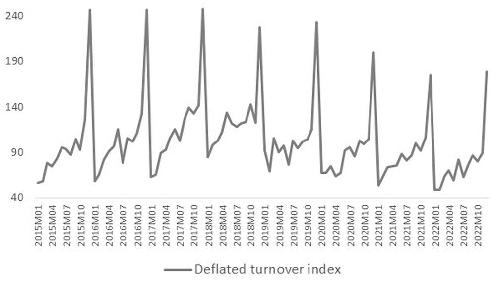
Monthly index of deflated turnover.
We use the number of employees as an exogenous variable in the model because labor is a major input to the construction industry. Figure 2 shows the monthly construction employment index. Seasonality affects the demand for labor in the construction industry. Because the labor force is overused during high seasons of construction and underused in low seasons (Dagum and Cholette 2006), construction employment data show similar seasonal variations to production in the construction industry, unlike turnover. One can argue that the variable of hours worked provides a better estimate of productivity, as it also reflects calendar effect variations. However, the hours worked data in Türkiye are published on a quarterly basis. Employment data from SSI also has its own limitations. The major drawback of administrative data is the exclusion of informal employment. The labor force survey comprises both registered and unregistered employment, but detailed results by economic activity are only available on a quarterly basis as the sample size is insufficient to provide independent monthly estimates. Because our analysis of quarterly LFS data revealed an almost stable relation between informal and total employment, we assumed that this relation is also valid for monthly employment series obtained from SSI data.
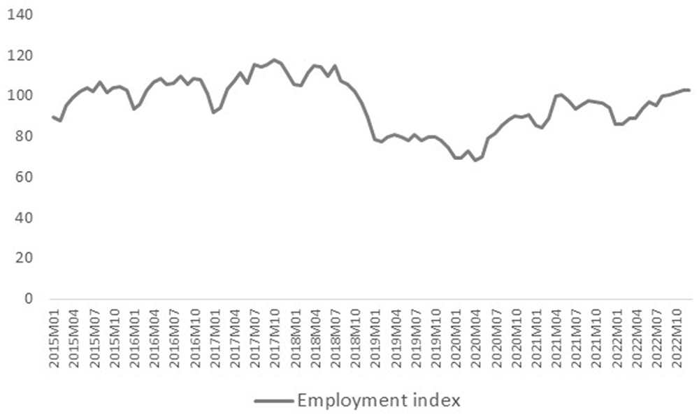
Monthly index of employment.
3. State-Space Modeling Approach
In this section, we present a new method for compiling monthly IPC using the SSM. The SSM has received increased attention in the production of official statistics in recent years, thereby proliferating studies on this subject: Pfeffermann et al. (1998) for Australian LFS; Silva and Smith (2001) for Brazil LFS; Elliott and Zong (2019) for UK unemployment statistics; Van den Brakel and Krieg (2009, 2015) for Dutch unemployment statistics; Tiller (1992) and Pfeffermann and Tiller (2006) for US labor statistics; Bisio and Moauro (2018) for Italian quarterly national accounts; Labonne and Weale (2020) for UK business sector output; and Balabay et al. (2016) for the Netherlands Road Transport Survey. This study pioneers the SSM application for estimating production in the construction industry.
We apply modified forms of the Chow–Lin (CL) model and its extensions, the Fernández and Litterman models, which are widely used by NSIs. We compare four alternative models—three assuming constant labor productivity and one assuming time-varying labor productivity.
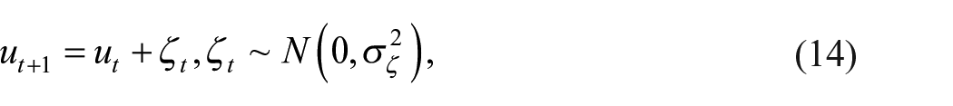
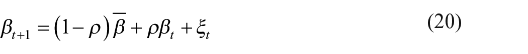
The general form of a linear Gaussian SSM is specified by two equations: the measurement equation (also known as the signal or observation equation) and the state (or transition) equation. The measurement equation provides a link between the (p × 1) vector of observable variables
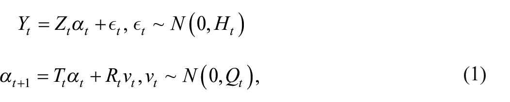
where
The main variables used in the models are
Notably,
3.1. SSMs Based on Constant Labor Productivity Assumption
In this section, we set up three SSMs, which are modified versions of the regression-based CL, Fernández, and Litterman-type temporal disaggregation models.
3.1.1. Chow–Lin-Type Model
Chow and Lin (1971) proposed a linear regression model for temporal disaggregation.

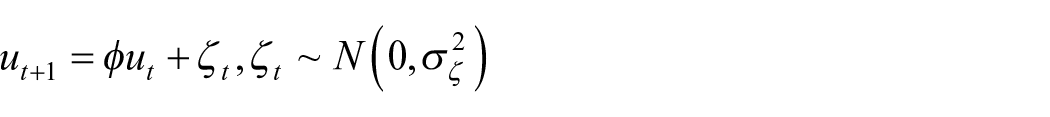
where

The disturbance series
Although the annual summation of the series implies a simple form of seasonal adjustment, the yearly series may still exhibit some calendar effects, including trading days and moving holidays that do not cancel within the year. In particular, the Ramadan and Sacrifice holidays, which are moving religious holidays in Türkiye, might substantially impact the number of working days in a month and the effect varies from year to year. Therefore, we have included the composite calendar regressor used by Turkstat in the seasonal adjustment process in the model given in Equation (3). This regressor is based on the number of effective working days in a month; therefore, it does not include the weekend or fixed national and moving holidays.

where

As previously stated, due to its seasonal bias, the deflated monthly turnover variable cannot be directly utilized as a proxy for the IPC. To overcome this issue, signal variable

Substituting

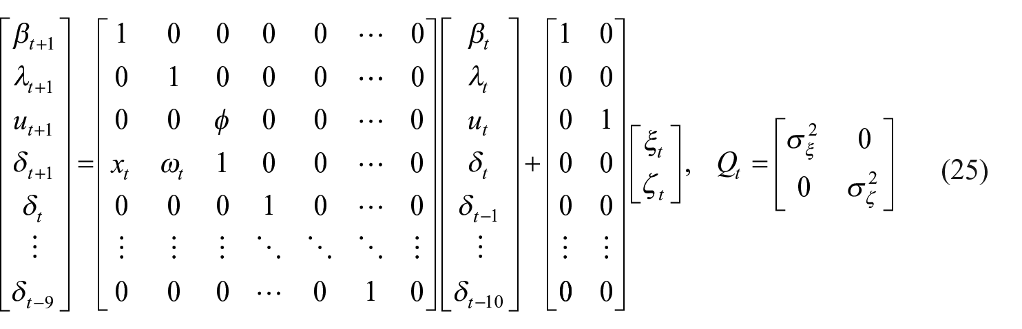
We can transform the observation Equation (9) into an equivalent minimal representation by defining the state variables for all lagged terms of the unobserved IPC as follows:

where
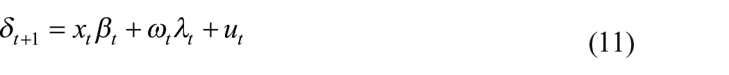
Hence, the aggregation constraints are satisfied by the observation equation. Once the model is estimated, the monthly IPC can be obtained indirectly using the number of employees, the smoothed estimates of labor productivity, and disturbance series (see the parenthesis in Equation (10)), or the lagged values of the IPC can be obtained directly from the smoothed estimates of the state variables,
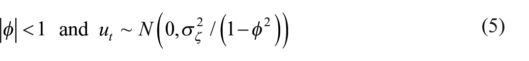
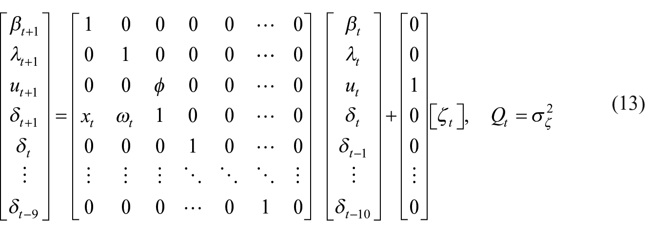
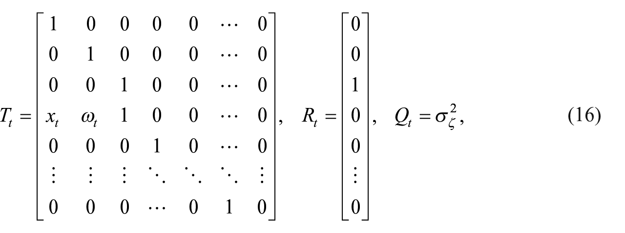
The state-space representation of the CL-type model is as follows:

where
The state transition equation is as follows:
3.1.2. The Fernández-Type Model
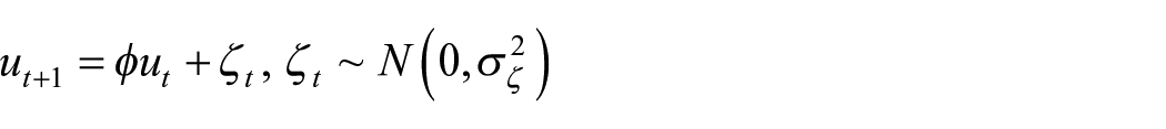
Fernández (1981) offered to extend the original CL’s AR(1) approach to the integrated model, where the error term follows a random walk process.
The state-space representation of the Fernández-type model is as follows:

The system matrices
The system matrices are the same as the CL-type model except for
3.1.3. The Litterman-Type Model
Litterman (1983) proposed a model where the disturbance term follows the ARIMA(1,1,0) process on the grounds that Fernández’s random walk model may not remove all the serial correlation.
The state-space representation of the Litterman-type model is as follows:

The system matrices
3.2. SSM Based on Time-Varying Labor Productivity Assumption
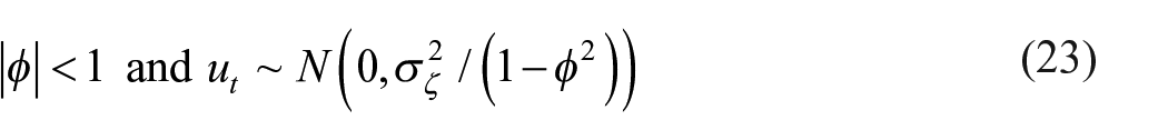
If the relationship between two economic variables is time-varying, employing a model with a constant parameter would constitute a specification error. In this case, the estimator will be inefficient, and the estimate of error variance usually is downward-biased (Rosenberg 1973b, 399). Given that the labor–output relation is affected by changes in capital intensity and total factor productivity, assuming that productivity is constant over time seems unreasonable. Therefore, in this section, we propose a model in which the labor productivity coefficient is allowed to vary stochastically over time.
The time-varying coefficient models were introduced into the literature in the 1970s including Swamy (1971), Cooper (1973), Rosenberg (1973a, 1973b), and Cooley and Prescott (1976), among many others. In the existing literature, stochastically varying regression parameter models are generally assumed to follow one of three processes: a random process, a random walk process, and a first-order Markov process or more generally an ARMA process (for a survey for these models, refer to Rosenberg 1973a).
Rosenberg (1973b) proposed a model in which the time-varying coefficients follow a first-order autoregressive process, as follows:
While the term If
If

If

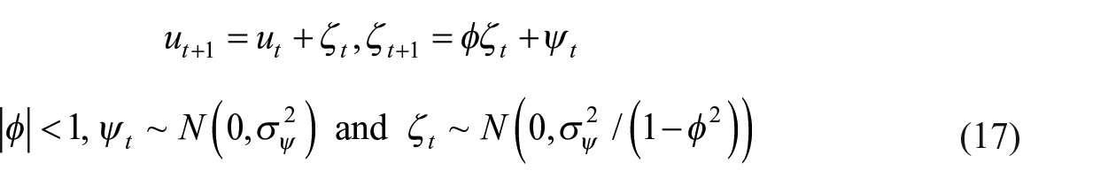
Perhaps the most widely used specification for a time-varying coefficient in empirical studies is the random walk model, as it is easy to implement, requires minimal information, and performs well for many datasets. According to Engle and Watson (1987), for most economic variables, the process should have a unit root and evolve slowly. Long-run productivity is more likely to evolve in a smooth and persistent manner over time. Therefore, we assume that the model representing the dynamics of productivity is the random walk model.
The unobserved monthly IPC with time-varying productivity is defined as follows:

where
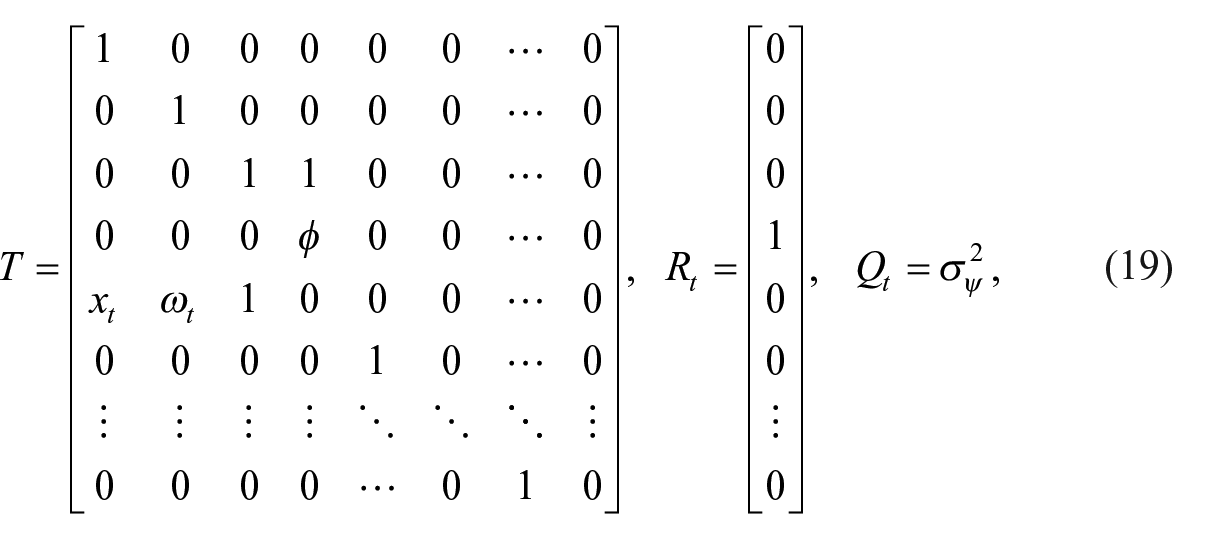
Consequently, in the SSM model based on time-varying productivity (hereinafter TV-CL), all equations are the same as the CL-type model in the previous section, except that the disturbance term

The state transition equation is as follows:
The models presented in this paper were estimated using SSpace object module of EViews software package. A quasi-Newton algorithm, the BFGS (Broyden–Fletcher–Goldfarb–Shanno) was used as the optimization method. Smoothed estimates were obtained from a fixed interval smoothing algorithm. State variables were initialized with nondiffuse initialization. The initial values of disturbances were set to zero, and the initial value of productivity in the TV-CL model was set to 1. The initial conditions of the covariance matrices, were applied based on the specifications outlined in the aforementioned models.
4. Empirical Results
4.1. IPC Estimates
Figure 3 presents a comparative display of the IPC estimates obtained from SSM. Notably, the wider confidence intervals for the CL-type and Fernández models indicate a higher degree of uncertainty compared to the TV-CL model and Litterman type models. All IPC estimates are very close to each other and follow a seasonal pattern similar to the employment series used as a related variable in the models. They also reflect nonseasonal movements embedded in deflated turnover data. This is because the information at the sub-annual (monthly) frequency is obtained from the number of employees and the moving sum of deflated turnover data.
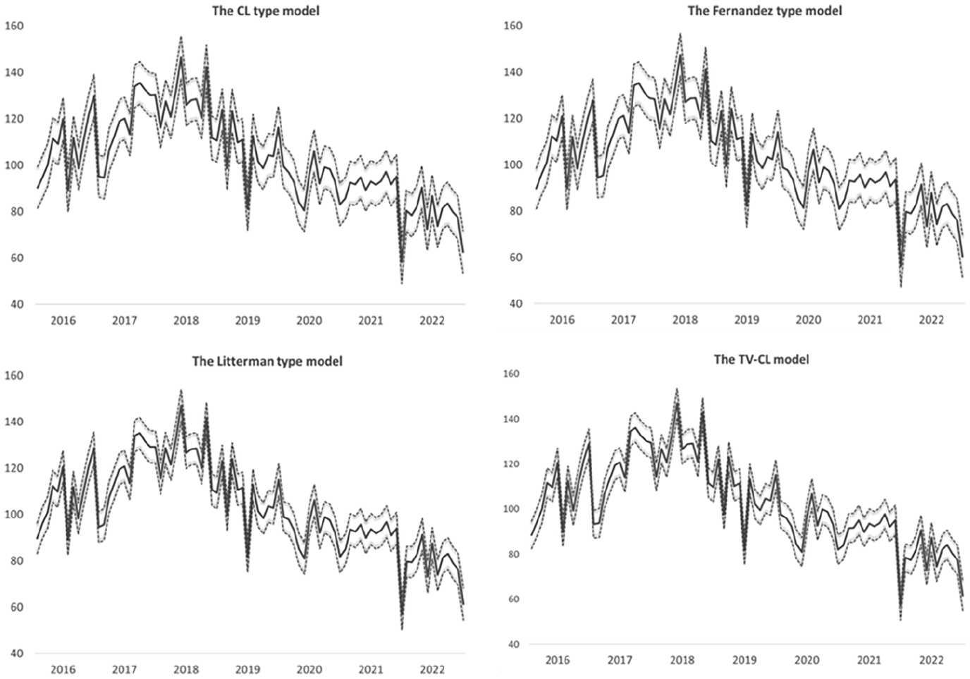
IPC estimates with confidence intervals. Solid lines show IPC estimates and dashed lines show corresponding ±2 standard error bands.
4.2. Time-Varying Labor Productivity Estimate
As mentioned before, the model representing the productivity dynamics is assumed to be the random walk model. Figure 4A presents the smoothed estimate of labor productivity obtained from this model. The annual productivity coefficients were calculated from the original annual data to evaluate how well the local-level model fits the real situation. These coefficients were derived by dividing the original annual turnover index by the original annual employment index. The annual productivity coefficients from the SSM are then compared with those from the original data. Figure 4B illustrates the annual productivity coefficients derived from the state-space model (SSM) are remarkably close to those calculated directly from the original data, highlighting the effectiveness of the random walk model in capturing the labor productivity dynamics.
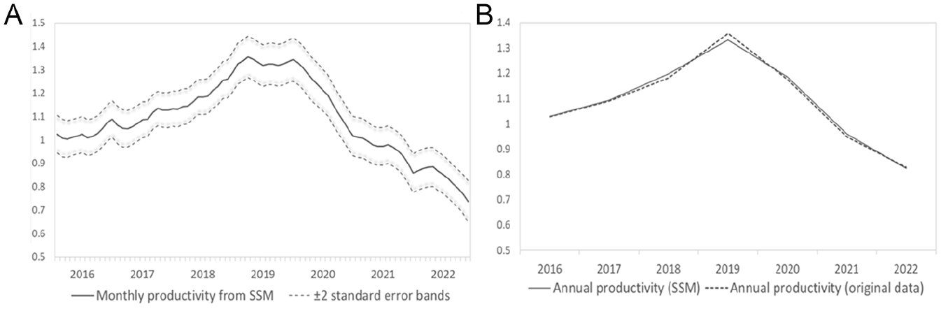
Comparison of labor productivity estimates: (A) Monthly labor productivity estimates from SSM and (B) Comparison of annual labor productivity estimates.
4.3. Model Selection
Table 1 provides maximum likelihood estimates of hyperparameters and model selection criteria for alternative model specifications. While the constant productivity value is around 1 for the CL-, Fernández-, and Litterman-type models, time-varying productivity for the TV-CL model is 0.71, which is the last estimate of
Estimation Results of Various Models.
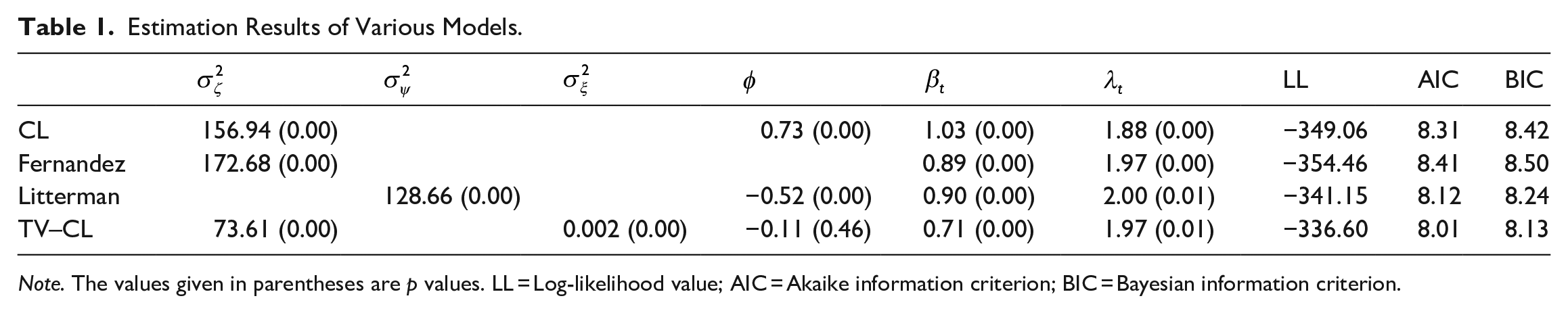
Note. The values given in parentheses are p values. LL = Log-likelihood value; AIC = Akaike information criterion; BIC = Bayesian information criterion.
Table 2 provides standard residual diagnostics for standardized smoothed disturbances to check the validity of the assumption that these disturbances are normally distributed without serial correlation. Augmented Dickey–Fuller (ADF) test statistics are used to identify whether disturbances exhibit stationarity. The Jarque–Bera test results show that the normality assumption is satisfied for the models based on constant labor productivity at the 5% significance level, while for the TV-CL model, normality is not satisfied. While Q statistics and autocorrelation values at lag 1 for the Litterman-type model are satisfactory, the CL- and Fernández-type models show the presence of first-order autocorrelation in their residuals. Q(12) statistics for the models based on constant labor productivity indicate a violation of the most important assumption of independence. On the other hand, the null hypothesis of independence cannot be rejected at the 5% significance level for the TV-CL model at lags 1 and 12. The ADF test results show that disturbances for the CL-type model have a unit root, whereas the TV-CL and integrated models satisfy the stationarity assumption. In conclusion, the diagnostic tests summarized in Table 2 reveal that the Litterman-type and TV-CL models outperform the CL- and Fernández-type models.
Diagnostics Tests for the Standardized Smoothed Disturbances of Various Models.
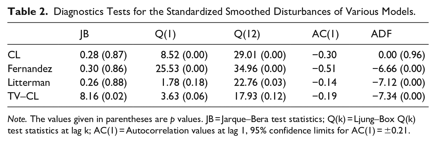
Note. The values given in parentheses are p values. JB = Jarque–Bera test statistics; Q(k) = Ljung–Box Q(k) test statistics at lag k; AC(1) = Autocorrelation values at lag 1, 95% confidence limits for AC(1) = ±0.21.
4.4. Revision Analysis
Model based estimates of official statistics are always subject to certain revisions, irrespective of the revisions to the original input data in the model. In the production process, the monthly published IPC figures are obtained from a real-time analysis based on the most recent data. When a new observation is added to the series, the previously published figures will be revised, as the model parameters will be re-estimated each month based on the available series observed up to this period. The more frequent and larger the revisions, the more damaging the reliability of statistical data from the user’s perspective. Therefore, comparing the revision performances of the models will serve as a valuable guide for selecting the most suitable model.
Figure 5 illustrates the concurrent estimates of the models for the last thirty-six months. These IPC estimates were obtained indirectly using the employment index and smoothed state estimates, as shown in Equation (10). In 2020, when the COVID-19 pandemic hit the construction industry, the revision amount for all models was obviously higher than in the latter period. The erratic changes observed in both the employment and turnover series during this period caused the model parameters estimated for the consecutive months to change drastically, which resulted in larger updates to the initially published figures. While the TV-CL model performed slightly better than others in the period 2020 to 2021, it performed similarly to the Litterman- and Fernández-type models in 2022. Meanwhile, the CL-type model underperformed than other models during the entire period.
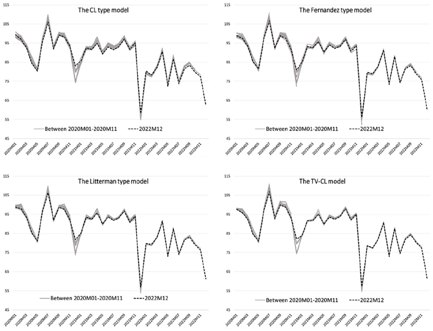
Concurrent estimates of the models for the period 2020:01 to 2022:12. Gray lines represent concurrent estimates spanning from January 2020 to November 2022. The dashed line indicates the IPC estimate for December 2022.
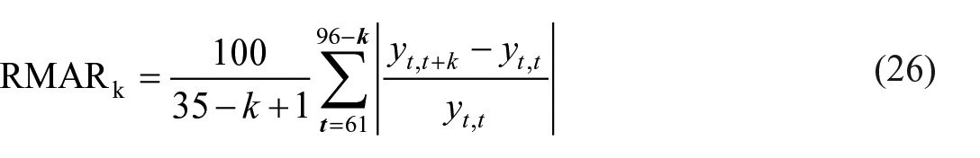
In order to evaluate the performance of the models, we consider three basic descriptive revision measures: relative mean absolute revision (RMAR), mean absolute revision (MAR), and root mean square revision (RMSR). If
We use RMAR to find the revision size for k steps in percentages in the IPC estimate levels. The revised IPC estimates are calculated starting from the sixty-first month, January 2020 to the ninety-sixth month, December 2022 as follows,
We used MAR and RMSR to find the revision size in the monthly (month-on-month) and annual (year-on-year) growth rates.
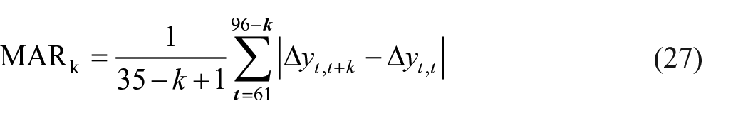
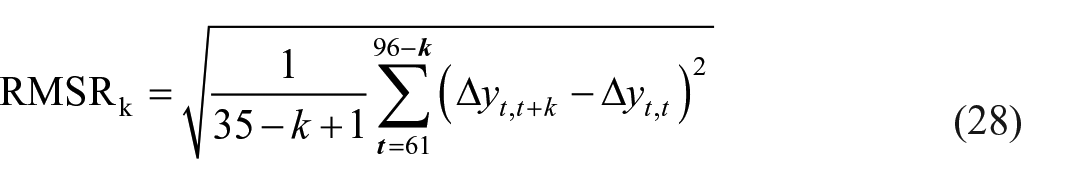
where Dyt represents the growth rate. While the monthly growth rate was calculated from the formula
The results for each step from one month to four months and for the twelve-month step, where we expect the most revisions, are presented in Table 3. The last column of Table 3 summarizes revision measure, demonstrating the overall performance of the models, which is obtained by averaging the revisions calculated for each
Revision Table for the Period 2020:01 to 2022:12.
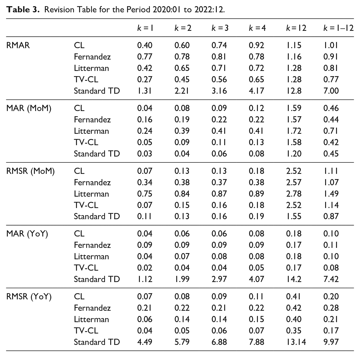
Furthermore, we utilized the standard temporal disaggregation method to determine whether the MTD approach can reduce the total revision sizes. In this case, we used the standard CL method, which is widely used by NSIs to derive monthly IPC using annual frequency turnover series rather than moving sums. We found that revision levels were indeed quite high, especially in terms of the annual growth rates and level of the series for
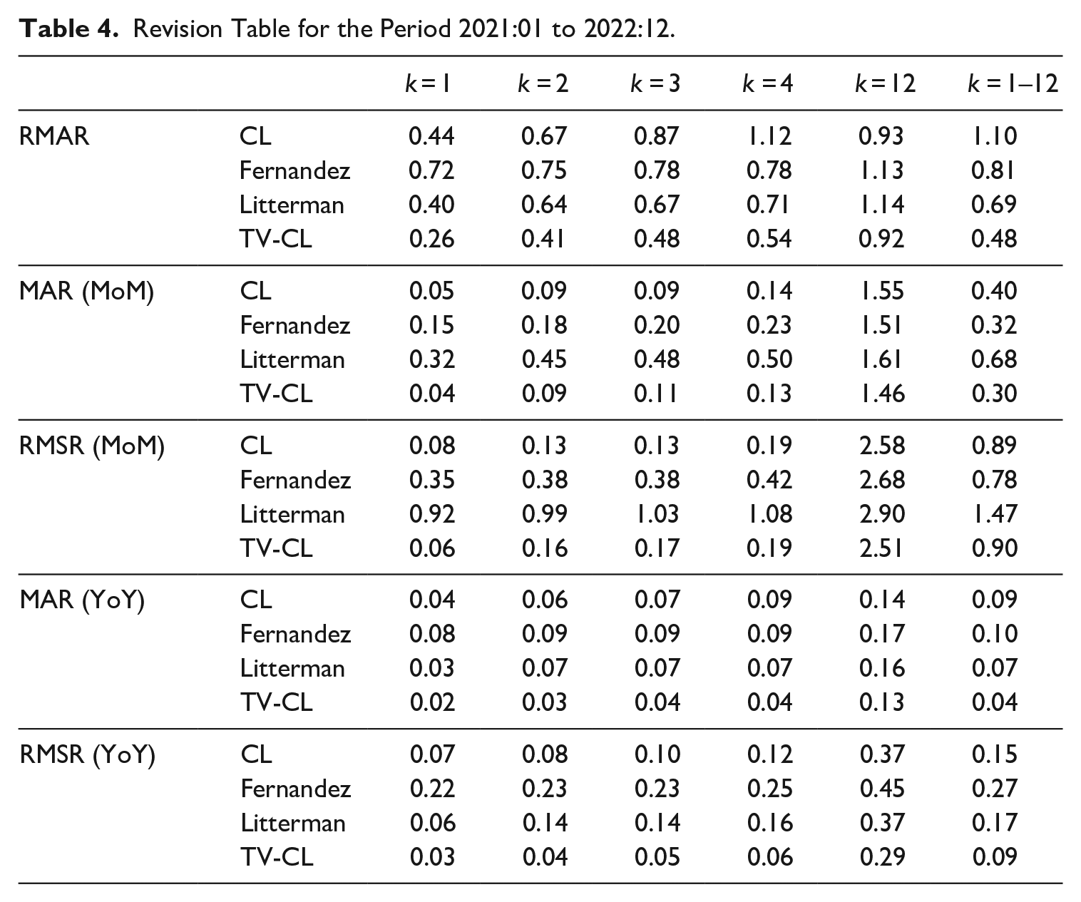
If the 2020 is excluded from the analysis, revision sizes are generally smaller than those in the previous table (Table 4). Only the CL-type model performs slightly worse than before considering RMAR. The TV-CL model outperforms the others for all revision measurement criteria except for RMSR (MoM), where the Fernández-type model performs better. The Litterman model underperforms the others in terms of revisions to monthly growth rates, as before. Therefore, the performances of the models are observed to be quite similar to those of our previous findings.
Revision Table for the Period 2021:01 to 2022:12.
5. General Discussion of Modified Temporal Disaggregation
The primary motivation behind proposing the MTD is to deal with the reported lag-induced seasonal bias in the deflated turnover data. Traditional temporal disaggregation methods can serve the same purpose, but they produce large revisions, as demonstrated using the standard CL method. These methods are principally used to estimate high-frequency values from low-frequency data. However, the utilization of low-frequency annual data may result in a loss of valuable information regarding the time series characteristics of the economic data. Rossana and Seater (1995) empirically examined the effects of temporal aggregation and concluded that “Monthly and quarterly data are governed by complex time series processes with much low-frequency cyclical variation, while annual data are governed by extremely simple processes with virtually no cyclical variation” (Rossana and Seater 1995, 441). In our case, we already have monthly turnover series but cannot use them in their current form as they suffer from data quality issues mentioned before. In the MTD model, the complete loss of monthly information is prevented using annualized monthly data instead of low-frequency annual data. Therefore, the superiority of MTD over standard temporal disaggregation is not limited to producing lower revisions, but it also reflects in nonseasonal movements embedded in deflated turnover data as information at the subannual (monthly) frequency is obtained from employment and deflated turnover data.
This study considered the employment variable deterministically. Certainly, alternative models treating employment stochastically might be used to address the seasonal bias problem. For example, a bivariate model can be established in which turnover and employment follow separate basic structural time series models. Furthermore, these models can be designed in relation to each other within an SSM framework. Trend, seasonality, and irregular components of employment and deflated turnover could then be estimated, and the IPC could be derived by borrowing seasonality from employment. Thus, the new IPC might have the trend and irregular components of turnover and a seasonal pattern of employment. However, such a modeling approach does not guarantee consistency between the annual totals of the IPC and deflated turnover. Over time, the levels of these two series may diverge. To circumvent this problem, published monthly IPC figures can be benchmarked to yearly sums of deflated turnover at each year-end, which is another source of revision. Alternatively, an SSM could be constructed such that monthly IPC estimates satisfy temporal constraints automatically in a single step. These alternatives hold some disadvantages, such as computational complexity and estimation of the large number of parameters from a relatively short series. Therefore, generally preferable method is to adopt a modeling approach in a routine statistical production that does not require serious expertise and is easily implemented.
As Lucas (1976) argued with his famous critique, the parameters of traditional macro-econometric models are unlikely to remain constant in a changing economic environment. Therefore, this study also addresses the dynamic properties of productivity by incorporating a time-varying coefficient within the MTD model. Standard temporal disaggregation methods consider the relation between the related series
6. Conclusion
In recent years, NSIs have increasingly adopted administrative data sources to generate official statistics that are cost-effective, reduce the burden on respondents, and provide timely and detailed information. However, since these sources are not designed specifically for statistical purposes, data quality may be negatively affected by timing differences, classification, and coverage issues. In Türkiye, the main data that forms the basis for estimating output in the construction industry is the monthly turnover series obtained from VAT registers. Like other administrative data sources, tax registers have some limitations. The main weakness of this data is that the seasonal pattern does not reflect the actual seasonal pattern of production in the construction industry, as companies operating in the industry usually declare most of their taxes to the government at the end of the calendar year. In this study, we proposed four alternative SSMs to address the seasonal bias problem that arises in monthly administrative data. We developed modified forms of the CL-, Fernández-, and Litterman-type models by assuming constant labor productivity and the CL-type model by assuming time-varying labor productivity.
The monthly IPC figures were obtained by the temporal disaggregation of the rolling annualized totals of the deflated turnover using the number of employees as a related indicator. The results indicated that the MTD-generated new IPC estimates were superior in terms of the representation capability of real economic activities in the construction industry compared to an indicator directly based on the turnover series. To evaluate the quality of models, we considered the standard model selection criteria and residual-based diagnostics. The results revealed that the Litterman-type and TV-CL models outperformed the CL- and Fernández-type models. Although standard model comparison techniques provide some insight into selecting the best model, we need further analysis in order to see how well the models perform in real-time production. To this end, we compared the revision performances of the models using the concurrent estimates of the models for the last thirty-six months. Accordingly, the overall revision performance of the models was satisfactory, especially since the average revision size in annual growth rates was quite small for all models. The results indicated that the TV-CL model outperformed the other three models based on constant labor productivity on four out of the five revision measurement criteria. The Fernández-type model performed slightly better than the TV-CL model for monthly growth rates with respect to RMSR, which is more sensitive to outliers in the sample. Additionally, we applied the standard CL method to determine whether the MTD approach was effective in reducing the total revision sizes. The standard temporal disaggregation model yielded much larger revisions compared to the MTD, especially in terms of the annual growth rates.
Considering the statistical quality and revision performance of the proposed models, we found that the TV-CL model outperformed the other three models. While the SSM framework permits time-varying coefficients for explanatory variables, the existing empirical literature on regression-based temporal disaggregation often assumes these coefficients to be constant. If the relation between a low-frequency series and a high-frequency series is not stable over time, trying to model this relation rather than residuals (or besides the residuals) may yield more satisfactory results. The proposed SSM with a time-varying coefficient can also be applied to any standard temporal disaggregation problems. This can be readily achieved by constructing the signal variable from the standard annual totals instead of the rolling annual totals.
Footnotes
Author’s Note
The views and opinions expressed in this paper are those of the author and do not necessarily represent the official views of the Turkish Statistical Institute.
Funding
The author(s) declared that they received no financial support for the research, authorship, and/or publication of this article.
Received: June 2023
Accepted: March 2024