Sim-to-real transfer of adaptive control parameters for AUV stabilisation under current disturbance

Abstract

Learning-based adaptive control methods hold the potential to empower autonomous agents in mitigating the impact of process variations with minimal human intervention. However, their application to autonomous underwater vehicles (AUVs) has been constrained by two main challenges: (1) the presence of unknown dynamics in the form of sea current disturbances, which cannot be modelled or measured due to limited sensor capability, particularly on smaller low-cost AUVs, and (2) the nonlinearity of AUV tasks, where the controller response at certain operating points must be excessively conservative to meet specifications at other points. Deep Reinforcement Learning (DRL) offers a solution to these challenges by training versatile neural network policies. Nevertheless, the application of DRL algorithms to AUVs has been predominantly limited to simulated environments due to their inherent high sample complexity and the distribution shift problem. This paper introduces a novel approach by combining the Maximum Entropy Deep Reinforcement Learning framework with a classic model-based control architecture to formulate an adaptive controller. In this framework, we propose a Sim-to-Real transfer strategy, incorporating a bio-inspired experience replay mechanism, an enhanced domain randomisation technique, and an evaluation protocol executed on a physical platform. Our experimental assessments demonstrate the effectiveness of this method in learning proficient policies from suboptimal simulated models of the AUV. When transferred to a real-world vehicle, the approach exhibits a control performance three times higher compared to its model-based nonadaptive but optimal counterpart.

1. Introduction

Recently, there has been a growing presence of autonomous vehicles in various sectors of society (Hakak et al., 2023; Hanover et al., 2023; Wibisono et al., 2023). Whether it is cars, trains, warehouse robots, or delivery quadcopters, the field of autonomous vehicles is flourishing. This progress is driven by the desire to enhance productivity, accuracy, and operational efficiency, while also prioritising the safety of human operators and users. Although this trend is observed in various domains, there is a noticeable discrepancy in the development of underwater applications. Despite similar requirements for tasks such as offshore platform inspections, marine geoscience, coastal surveillance, and underwater mine countermeasures, most unmanned underwater vehicles still rely on remote operation or possess limited autonomy capabilities. This issue is even more pronounced in the context of small-sized autonomous underwater vehicles (AUVs). These vehicles are required to operate over large regions (from deep oceans to coastal and riverine regions), and over lengthy periods of time (extending from several hours to days before the possibility of human intervention) performing complex tasks such as search and rescue (Anderson and Crowell, 2005), underwater manipulation (Marani et al., 2009), pipeline and facility inspection operations (Gilmour et al., 2012), target following (Sun et al., 2015), and under-ice exploration (Barker et al., 2020), among others. Nevertheless, the autonomous control of underwater autonomous vehicles still presents several challenges. Developing robust control algorithms that can ensure the safe and efficient operation of underwater autonomous vehicles remains an ongoing area of research and development. The challenges still outstanding, that need to be addressed include (Chaffre, 2023):

• Unknown dynamics: fixed feedback control methods are prevented from achieving optimal performance due to waves and currents disturbance being difficult to describe precisely and whose characteristics vary over time. Moreover, changes in weather conditions impose a multiplicative factor in the component of the induced forces. The disturbance period will also vary with the vehicle speed and its orientation relative to the waves.

• Nonlinearity: the controller response at some operating points must be overly conservative to satisfy the control requirements at different operating points. This is not possible with a fixed controller determined by using local linearisation, which does not encompass the entire regime envelope.

• Thruster efficiency: even when being fully actuated, an AUV can become underactuated when its speed varies. This is especially true for hovering-type AUVs which use thrusters in place of steering fins to achieve manoeuvrability at low speeds. As forward speed increases, the effectiveness and efficiency of lateral thruster-induced movements are drastically reduced, making it impossible for the vehicle to account for pure lateral motions.

• System reliability: In the event of a decrease in thruster performance, the control system should possess the capability to detect such changes and activate a new control algorithm specifically designed to address the failures. Ideally, this alternative algorithm should be tailored to accommodate the degraded thruster performance and, if feasible, ensure the successful completion of the mission.

For these reasons, the present work assumes the standpoint of learning-based adaptive control methods, where machine learning algorithms are employed to compensate for the unknown aspects of a process while control over the known parts is ensured by using traditional methods. Here, the term ‘unknown’ means that these aspects are unmodelled either because we do not have the sensors to measure their underlying components or we do not have a model precise enough to effectively represent them. This research focuses on the control of manoeuvring tasks for AUVs, specifically the stabilisation of the vehicle at a fixed velocity and orientation. The AUV is assumed to be fully actuated and affected by external disturbances, represented by sea currents, which are considered non-observable variables in this research. The dynamics of an AUV can be described as a combination of its known and unknown components. To address this, the present paper builds upon our previous work (Chaffre et al., 2022b), whereby a novel deep reinforcement learning method was used to compensate for the unknown part of the plant, whereas a traditional PID controller was used to control its known part.

Reinforcement learning (RL) (Sutton and Barto, 2018), a subfield of machine learning (ML), focuses on the development of algorithms and techniques that enable an agent to learn the optimal sequence of decisions in an environment, aiming to maximise cumulative rewards. Rooted in behavioural psychology, RL emulates the learning process observed in trial and error, where the agent interacts with its environment and receives feedback in the form of positive or negative rewards. When applied to real robots, a major challenge in reinforcement learning is to successfully transfer policies, learnt from simulated environments, to the target domain. Although there have been significant advances in the development of Deep Reinforcement Learning (DRL), which extends RL by combining RL algorithms with deep neural networks improving the scalability and generalisation of methods, sim-to-real transfer remains a bottleneck (Zhao et al., 2020). The focus of the present paper is on the experimental evaluation of transferring policies that were first learnt by a DRL agent in a virtual environment to a physical AUV under various disturbance regimes. The DRL algorithm used in this work is the Soft Actor-Critic with Automatic Temperature Adjustment algorithm (Haarnoja et al., 2019), which was combined here with the Biologically Inspired Experience Replay (BIER) method introduced in Chaffre et al. (2022b). BIER is a replay mechanism (Lin, 1992) that incorporates two distinct memory buffers: one that stores and replays incomplete trajectories of state-action pairs and another that prioritises high-quality regions of the reward distribution. BIER, as employed in this study, was utilised to determine the control parameters for an AUV.

The control policies were learnt on a virtual AUV modelled on the BlueROV 2 Heavy Remotely Operated Vehicle (ROV) before being subsequently transferred to its physical ROV counterpart (Blue Robotics Inc, 2017a). The physical vehicle in this case was operated in autonomous AUV mode rather than its native ROV mode. For the rest of the paper, it will therefore be denoted as an AUV. The experiments were conducted in a large indoor test tank environment where two thrusters aimed towards the vehicle were specifically employed to create current disturbances.

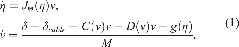
The experimental environment is depicted in Figure 1(b) where the task of underwater multi-station keeping under varying current disturbance by the AUV was conducted in this work. To that end, we proposed operating within the poles domain of the control law, as it offers greater ease in defining constraints for control performance requirements compared to working in the space of gains. The management of the resulting high-dimensional continuous state and action spaces was effectively addressed through the utilisation of Maximum Entropy Deep Reinforcement Learning (Ahmed et al., 2019). Maximising the entropy helps the agent to build a more robust policy by forcing the exploration of suboptimal trajectories, resulting in improved generalisation capabilities. Process uncertainty was further taken into account by building a stochastic policy. The effect of partial observability of the process is amplified since, in the present context, the current disturbance is not available. This issue was alleviated by considering an augmented state-space representation of the AUV process where the IMU feedback was incorporated into the state vector to indirectly capture the effect of the disturbing forces, allowing the DRL algorithm to compensate for it. Finally, the Sim-to-Real Transfer of the policy was achieved by reducing the distribution shift problem via an improved Domain Randomisation method (Tobin et al., 2017).

Figure 1.

Illustration of the setup for the experiments. We collected over 180,000 timesteps from the experiment to evaluate the predictive model, emphasising approximately 280 min of operating time. (a) The camera is positioned facing downward, precisely aligned using floor mounting points. (b) The image shows the two thrusters generating water displacement throughout the entire tank.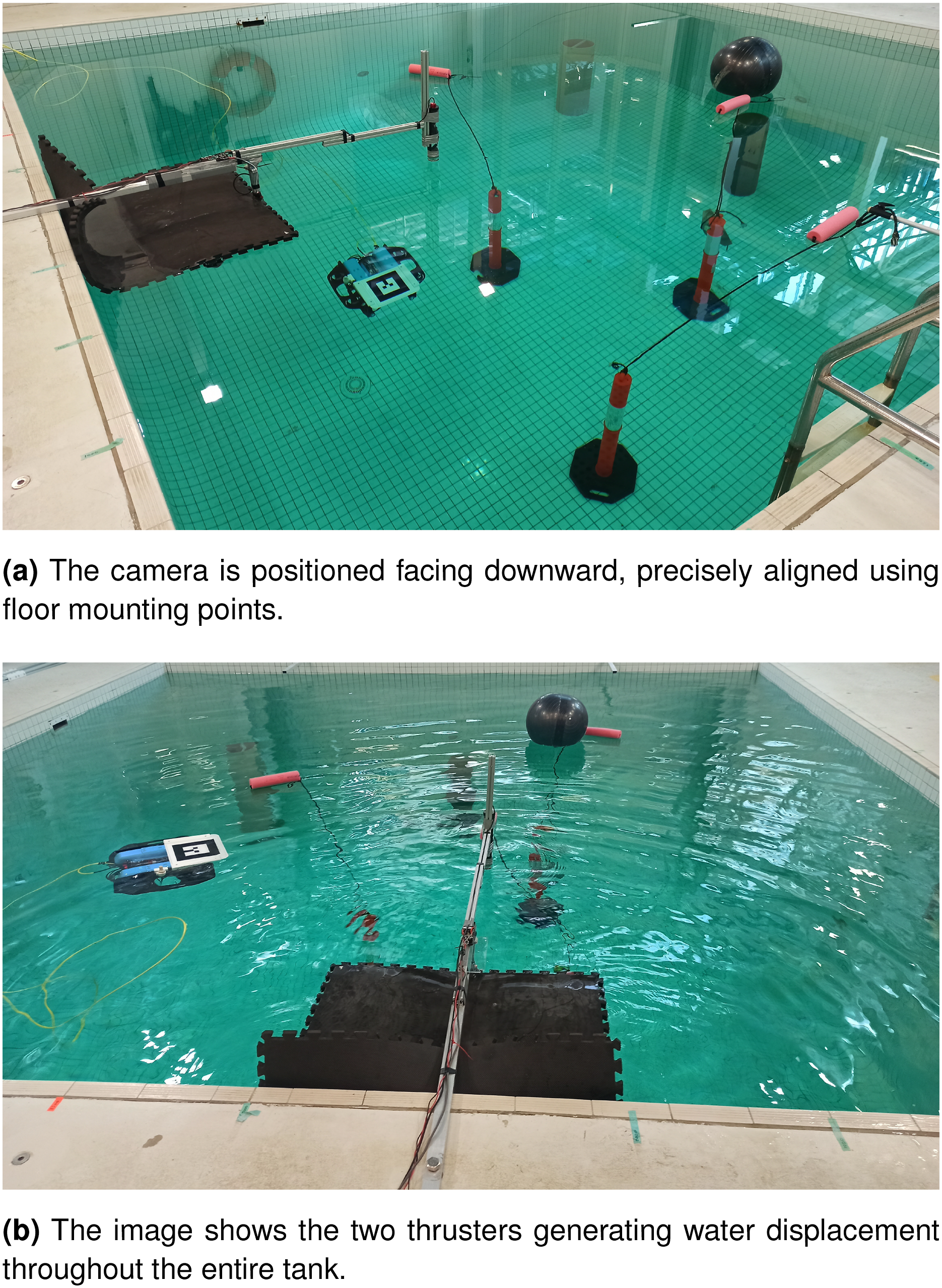

The main contributions of this work are the following:

(A) The experimental evaluation of a learning-based adaptive controller, and its nonadaptive (but optimal ¹ ) model-based counterpart, on a real platform. As a consequence of these experiments we showed that, despite being trained on a simulated vehicle model distinct from the physical one, the proposed method presented a superior performance at regulating the AUV when transferred to the real platform compared to the model-based approach.

(B) The design of a learning-based adaptive control structure for the given task, where control parameters dynamically adjust to accommodate process variations. This approach aims to achieve improved convergence stability and minimise steady-state error when compared to the robust version of the same control structure.

(C) The investigation of the relationship between the complexity of the source and target domains. This revealed that training directly in the highest complexity environment did not adversely impact long-term training performance, as long as the agent systematically encounters every level of complexity in proportion.

Earlier works investigating the use of DRL for adaptive control of AUVs have often focused on the design of purely model-free adaptive controllers. In the next section, we begin by identifying the related work in this area along with the challenges associated with the underwater environment.

2. Related work

Real-world systems are often characterised by nonlinear dynamics and uncertainty in their motion equations, parameters, and system measurements. Learning-based adaptive controllers offer a promising approach to address this challenge by leveraging model-free learning algorithms to approximate the unknown parts of the system model (f₂) and tuning control parameters for the desired behaviour (Benosman, 2017). Among the various learning techniques, Reinforcement Learning (RL) stands out as a prominent candidate for achieving this objective (Sutton and Barto, 2018).

RL formulates the control problem as a Markov Decision Process (MDP), represented by the tuple ⟨S, A, T, R⟩, where S denotes the set of possible states, A represents the set of actions that the agent can execute, T is the transition function defining the probabilities of reaching successor states, and R represents the reward function (Sutton and Barto, 2018). The RL process can be summarised as follows: in the initial step, at each timestep t, the agent chooses an action a _t ∈ A based on the current state s _t ∈ S. The execution of the chosen action results in a transition to a new state s_t+1 ∈ S, and the agent is rewarded with a scalar value r _t . This reward quantifies the quality of the action outcome according to a reward function R(s _t , a _t ). The overarching objective of RL is to maximise the expected future rewards attainable at each state. The agent continually updates the value associated with the selected action, refining the learnt policy based on the received rewards.

Deep Reinforcement Learning (DRL) extends the RL methods by utilising deep neural networks (DNNs) to approximate the functions defining the agent’s policy and state-action values (Sutton and Barto, 2018). DRL methods can be classified into three classes: Model-based, Value-based and Deep Policy Gradient (DPG) methods. In DPG methods, which are the main focus of this paper, the aim is to model and optimise the policy behaviour π directly which is denoted in this context as the actor. The policy is traditionally represented by a parameterised function with respect to θ and noted π _θ (a|s) (Sutton et al., 1999). The value of the reward function J(θ) depends on this policy and thus we can use various algorithms to optimise θ. The reward function is defined as the expected return and the parameters θ are optimised to maximise the reward function. Traditionally, the expected future return is represented by the state-action value function (known as the Q-value function) and its estimator is denoted as the critic. The combination of the two forms what is known as the Actor-Critic algorithm (Konda and Tsitsiklis, 1999) and the majority of DPG methods are based upon this structure where both estimators are simultaneously optimised. DPG methods are currently leading the application of RL in the field of robotic control systems because:

• They have better convergence abilities thanks to their off-policy formulation (Watkins and Dayan, 1992) which allows different policies to be used for exploration.

• They can be used in high-dimensional/continuous state and action spaces while model-based and value-based methods are not capable of tracking such spaces.

• They can learn stochastic policies which are more robust to process variations and provide better passive exploration abilities compared to their deterministic counterpart.

Nevertheless, DPG methods are also associated with high data complexity compared to the other class of solution methods. In DPG methods we are mostly choosing actions in a small area around the current best policy, making it easy to converge to a local minima or to overlook insightful regions of the state and action spaces. Therefore, when using a DPG method, it is essential to adopt superior exploration strategies such as an entropy loss term (Haarnoja et al., 2017) or a noise-based exploration (Fortunato et al., 2018; Plappert et al., 2018). A complete description of state-of-the-art DPG methods is presented in Weng (2018).

In a recent survey (Dulac-Arnold et al., 2020), the main challenges of applying DRL to physical robotic systems were listed, including the need for satisfying non-trivial environmental constraints, the high-dimensional (continuous) state and action spaces and the search for efficient solutions to multi-objective reward functions, when dealing with complex problems such as AUVs processes. Advances in DPG have led to the development of specialised algorithms, such as deep deterministic policy gradients (DDPG) (Lillicrap et al., 2016), twin-delayed DDPG (TD3) (Fujimoto et al., 2018), or the Soft Actor-Critic (SAC) algorithm (Haarnoja et al., 2018), that can handle high-dimensional continuous spaces more efficiently. In addition, Lyapunov stability with respect to DRL-based control systems is still not fully understood (García and Fernández, 2015). In fact, in our previous work in the context of AUV control (Kohler et al., 2022), we conducted a comparison of the Lyapunov stability between a learning-based adaptive PID controller and an adaptive PID controller. The latter had its parameters deliberately chosen to ensure adherence to the Lyapunov stability criterion. Our observations revealed that both controllers exhibited similar stability concerning vehicle state stability, as per the principles outlined in Lyapunov theory (Liberzon, 2005b). However, a significant contrast was observed in terms of the stability of the controller parameters. Another notable challenge stems from the partial observability and non-stationarity inherent in real-world environments. Particularly in the case of AUVs, the limited capacity for onboard sensors due to their small size poses difficulties. This limitation makes it challenging, and at times impossible, to measure process disturbances, further complicating the task of disturbance rejection.

Meeting these challenges has recently been the focus of much work in this area. The DDPG (Lillicrap et al., 2016) algorithm was used to learn the optimal trajectory tracking control of AUVs, where the control problem consists of keeping the error e = x − x _d between the actual trajectory x and the target x _d at zero (Yu et al., 2017). A loss function was defined to update the parameters of the actor network which includes Lyapunov stability components (Liberzon, 2005a). This approach was compared to a fixed-gain PID and the results indicate that the learning-based controller exhibited better performance in terms of tracking error. However, as the stability components were incorporated by an additional term in the actor loss function, there were no formal guarantees that the system would remain stable at all times. Learning-based adaptive control was investigated by Knudsen et al. (2019) in a station keeping task executed by an AUV under unknown current disturbances. The DDPG algorithm was used to control the position of a BlueROV2 platform in surge x and sway y combined to a PD control law that regulated the AUV position in heave z and orientation in roll ϕ, pitch θ and yaw ψ. The DDPG algorithm was used to learn a PD control law as a function of the vehicle position and velocity at previous timesteps. The training was performed within the Robot Operating System (ROS) Gazebo simulator (Quigley et al., 2009). The evaluation was conducted on a real platform in an indoor water tank and consisted of three scenarios: two of which had different desired pose definitions and the third assumed a 4-corner test. The first scenario consisted of changing one error state while in the second scenario, both error states were changed at the same time. The 4-corner test consisted of performing station keeping at the 4 corners of a rectangular trajectory. These experiments showed that the agent was able to complete the task under real conditions. The performance was, however, slightly worse in the real environment compared to the simulated one, especially for the most challenging task of a 4-corner test. More recently, Deep Imitation Learning (DIL) (Liu et al., 2018; Peng et al., 2018) and the TD3 algorithm (Fujimoto et al., 2018) were combined in Chu et al. (2020) for the design of a learning-based controller for an AUV (the combination of DIL and DRL was denoted DIRL). The idea of DIL is to apply some expert agent to generate examples of appropriate behaviours that are then used to perform the pre-training procedure of the DNNs in a supervised way. Then, the neural networks could be fine-tuned using the normal DRL framework under a reduced number of episodes. Comparisons were conducted between the proposed method, named IL-TD3 (a combination of DIL and TD3), to the original PID controller with and without current disturbances. This comparison was executed for two tasks: (i) constant depth and attitude control; and, (ii) depth trajectory tracking control. Results showed that, in the case where no disturbances were applied, both methods were able to solve the tasks; whereas, IL-TD3 exhibited a faster response and a lower overshoot, at the cost of a much higher thruster solicitation than the PID algorithm. Without disturbances, the trajectory performed by the IL-TD3 algorithm was almost identical to the reference one. The current disturbance was introduced by applying an additional torque in three directions, modelled using sinusoidal functions. In this case, IL-TD3 was able to complete the task with a satisfying tracking error, while the fixed PID controller displayed a large overshoot and oscillations with poor control performance. The advantage of their method was also demonstrated with physical tank experiments on the BlueROV2 platform. Upon transferring the policy network from simulation to the real-world scenario, simulation being the sole training environment, it exhibited superior performance in depth trajectory following when compared to a fixed optimal PID controller.

We can observe that two major trends are dominating the field of adaptive control of AUVs: direct and indirect approaches. In the former case, the parameters of the controller are adjusted directly using DRL, whereas in the latter case, the adjusted control parameters are the result of solving an optimisation problem where the state and/or unknown parameters of the process are first estimated and then used to compute the associated optimal parameters.

In most cases, these approaches are applied to classical model-based control structures such as the PD or PID control laws. The objective is then to adjust the parameters of these control structures (their gains) according to process variation, using DRL algorithms such as TD3 and the DDPG algorithms. These deep policy gradient methods build deterministic actors and do not take into account the entropy term from the maximum entropy reinforcement learning framework (Ahmed et al., 2019). Most of these works use the original experience replay mechanism (Lin, 1992), with a few exceptions, such as Wang et al. (2018) where the past experiences of the agent are selected based on different control constraints and stored in separate replay buffers. By using only selected samples to update the actor, the resulting policy displayed a more robust behaviour with respect to the imposed constraints.

In contrast, we demonstrate that our method is capable of learning satisfactory behaviour from a suboptimal model of the real vehicle, irrespective of process variations. Furthermore, previous applications of DRL for adaptive control AUVs generally do not exceed the performance of state-of-the-art maximum entropy algorithms, such as SAC (Haarnoja et al., 2018), even though they may offer other advantages, such as improved learning stability and reduced fine-tuning.

Our simulations illustrate how learning stability is enhanced through the proposed Domain Randomisation (DR) technique combined with the Automatic Temperature Adjustment mechanism. In our experiments, we demonstrate that our learning-based adaptive controller significantly outperforms its nonadaptive optimal model-based counterpart.

3. Sim-to-real transfer of adaptive control parameters for AUV stabilisation

The goal of this study is to introduce an adaptive control architecture that integrates Deep Reinforcement Learning (DRL) and model-based control. This architecture is designed to dynamically adjust its parameters in response to unmeasured current disturbances. The essential components of this analysis are summarised below.

3.1. Task description

The problem domain considered in this work is the control of manoeuvring tasks for AUVs. The primary control objective is to achieve multi-station keeping, which entails stabilising the AUV successively at various spatial setpoints, each defined by a specific position and orientation for a predetermined duration. The stabilisation is considered successful if, over a specific amount of time, the distance to the target position and orientation remains below a predefined threshold.

3.2. Simulated and real-word robotic systems

For the concept of transfer learning to be demonstrated, both simulated and real-world testing platforms were used.

We used the UUV simulator, a Robotic Operating System (ROS)-based environment commonly applied for training of the policy of agents via RL (Manhães et al., 2016). It allows the introduction of disturbing forces which, when incorporated into the simulations, have a realistic physical impact on the robots and fluid dynamics. The sea current disturbance (which is the main focus of this study) is modelled in the simulator as a uniform force acting over the entire simulated environment. This force is represented by a linear velocity, v _c (in m.s⁻¹), a horizontal angle h _c and a vertical angle j _c (measured in radians). These characteristics can be changed at any time in the simulations through ROS-based callbacks or directly through Python/C++ scripts. ROS (Quigley et al., 2009) is a very popular system in research robotics allowing the rapid development of robotic systems by the combination of small and simple programs called nodes that communicate information via topics.

For this project, the chosen hardware platform was a modified Blue Robotics BlueROV 2 Heavy configuration (Blue Robotics Inc, 2017a). The BlueROV is a low-cost compact ROV that has been applied in a variety of situations ranging from hobbyist use to applications in aquaculture and inspection of marine objects. The heavy configuration adds extra thrusters making the vehicle over-actuated with a total of eight thrusters, allowing control over all its six axes.

Flinders University’s BlueROV has been modified to include an ALVAR AR tag (VTT Technical Research Centre of Finland Ltd, 2019) for pose measurements, by an externally mounted camera, in addition to the acceleration and rotational rate from the Pixhawk Flight Controller and depth from the onboard pressure sensor. These measurements are fused by an Extended Kalman Filter (EKF) system estimating the BlueROV’s 6 degrees of freedom (DoFs) pose and velocities (cf. Section 8). This vehicle has also been modified to use ROS.

The physical model of the AUV, which encompasses the known part of the controller (f₁), can be summarised using the state-space representation described below (Fossen, 1991; Yang et al., 2015):

$\begin{array}{cc}\hfill & \dot{\eta }=J_{\mathrm{\Theta }}(\eta )\nu ,\hfill \\ \hfill & \dot{\nu }=\frac{\delta +{\delta }_{\mathit{cable}}-C(\nu )\nu -D(\nu )\nu -g(\eta )}{M},\hfill \end{array}$

(1)

where η and ν are position and velocity vectors, respectively, δ is the control force vector, and δ _cable represents the forces from the cable attached to the AUV. The control vector u is obtained using the equation δ = T(α)Ku, where $\mathbf{T}(\alpha )\in {\mathbb{R}}^{n\times r}$ is the thrust allocation matrix, K is the thrust coefficient matrix, δ is the control force vector in n DOFs, and $\mathbf{u}\in {\mathbb{R}}^r$ is the actuator input vector. For this class of process, a PD-type control structure is traditionally exploited thanks to its suitability for naturally delayed responses as exhibited by an AUV. Nevertheless, the AUV is subject to an additive but unknown current disturbance which can be modelled as:

$u_{\mathit{adp}}=u+u_{\text{current}}.$

(2)

In this context, despite u _current being unknown, the addition of an integral term could ensure convergence to the steady-state as t → ∞ despite the presence of a non-varying current disturbance, but at the cost of additional increased instability.

3.3. Evaluation

Once trained in a simulated environment, the resulting policy was evaluated in the real world against again its model-based counterpart defined in Wu (2018) which is a nonlinear model-based PID controller. In particular, it consists of using the nonlinear dynamics model of the vehicle equation (1) to produce a 6-DoFs predictive force and a model-based PID controller is used to provide a corrective force in 6-DoFs to adjust the error in the model. The parameters of the PID controller are fixed and were obtained using the Ziegler-Nichols tuning method (Ziegler and Nichols, 1942). The evaluation was split into two scenarios: with and without varying current disturbances. Since both controllers were based on the same PID control structure, it is fair to compare them as they produce analogous control inputs. The detailed descriptions of the simulations and evaluation are given in Section 8.

The following section outlines the control design, commencing with the model-based component of the proposed learning-based adaptive controller.

4. PID-based control structure

4.1. PID description

The state of the vehicle described in Section 3 at the timestep t denoted as X _t is defined by its Cartesian position and Euler orientation ${\mathrm{X}}_t={[x_t{y}_t{z}_t{\varphi }_t]}^T$ (yaw angle for its orientation). A setpoint is defined as ${\mathrm{X}}_w={[x_w{y}_w{z}_w{\varphi }_w]}^T$ and the error vector on the setpoints is defined as E _t = X _t − X _w . Here, given the characteristics of the vehicle, the roll and pitch angles of the AUV are not controlled, as they need to vary for the vehicle to perform sway and surge movements, whereas these parameters stabilise to 0 when performing station keeping given the centre of buoyancy of the AUV. The control objective is therefore to minimise the Euclidean distance d _t between the AUV and the setpoint:

$d_t=\sqrt{{(x_w-x_t)}^2+{(y_w-y_t)}^2+{(z_w-z_t)}^2+{({\varphi }_w-{\varphi }_t)}^2}.$

(3)

The task of station keeping can be achieved if the following control objective is met:

$\forall t^{\prime }\in [t-\varsigma ,t],\Vert {\text{E}}_{t^{\prime }}{\Vert }_{\infty }<d_{\mathit{reached}},$

(4)

where d _reached is the predefined threshold value on the errors under which the setpoint is considered satisfied and ‖ ⋅ ‖ _∞ is the vectorial Chebyshev norm. This class of control objective is used in various AUV missions, such as autonomous docking or underwater inspection.

This work assumes that the state of the AUV is observable and controllable as we have sensors which provide measurements of its linear and angular velocities as well as its orientation in terms of Euler angles. The following state-feedback controller, equivalent to a PID, can therefore be determined:

$u_t=-k_p{\text{E}}_t-k_i{\text{Z}}_t-k_d{\text{V}}_t,$

(5)

where ${\text{Z}}_t={\int }_0^t{\text{E}}_{\tau }d\tau$ , V _t = E _t d/dt, and k _p , k _i , $k_d\in {\mathbb{R}}^{+}$ are the control gains. Nevertheless, only the AUV’s inertial measurement unit (IMU) feedback is available, and the characteristics of the current disturbance cannot be directly measured or estimated. In this context, the performance of the PID is variable against these nonlinearities. Traditionally, a linear representation of the nonlinear dynamics of the AUV would be made and, at specific points, they could be linearised as a series of linear functions across the operating range. For each linear function, a PID controller with different gains could be determined and an interpolating function could be used for the transition between operating points. This method is known as Gain Scheduling (Clement et al., 2005) and the further the AUV diverges from the point of linearisation, the more ineffective the PID control will be. However, as in this work, the current disturbance is not available, it is impossible to determine the scheduling regimes. For this reason, we propose a learning-based adaptive pole-placement formulation applied to the PID control structure, as described in the next section.

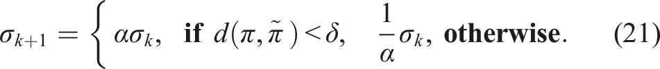
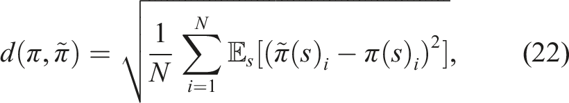
4.2. Adaptive PID tuning strategy

In practice, for the PID controller equation (5) to be effective, anti-windup compensation on the integral term and low-pass filtering on the derivative term have to be added:

$u_t=k_p{\text{E}}_t+\min (k_i{\text{Z}}_t,{\widehat{u}}_t)+k_d\left((1-r){\delta }_{t-1}+r{\text{V}}_t\right),$

(6)

where ${\widehat{u}}_t$ is the maximum control input that can be sent to the AUV speed controllers, $|u_t|<{\widehat{u}}_t$ , $r=e^{-T_s/T_f}=e^{-4}$ (De-Larminat, 2009) is a smoothing factor, and δ_t−1 is the output of the filter at the previous step. For an n ^th order linear system, the minimum requirement for output boundedness is for its poles to be placed in the complex left half-plane. Candidates for eigenvalues are determined as solutions of λ³ + λ²k _d + λk _p + k _i = 0. To maintain the gain space dimension, the pole value candidates ${\tau }_i\in {\mathbb{R}}^{+}$ are defined as follows:

${\lambda }_1=\frac{-1}{{\tau }_1};{\lambda }_2=\frac{-1}{{\tau }_2};{\lambda }_3=\frac{-1}{{\tau }_3}.$

(7)

The controller gains are determined through a resolution and transformation process explained in detail in Chaffre et al. (2021). By considering the design in equation (7), the bounds for the controller parameters can be defined based on control constraints that are easier to derive in the pole domain. In this case, for any τ _i > 0, the poles of the feedback loop are placed on the x-axis of the complex left half-plane (Chaffre et al., 2021). However, it is important to note that the resulting nonlinear system requires Lyapunov methods to conduct a stability analysis (a complete methodology to perform such analysis is provided at the end of this section). The upper bound of the poles λ _max is then determined as:

${\lambda }_{max}=\frac{\ln (\chi )}{\varsigma },$

(8)

where ς is the desired time after which we want the system outputs to remain within χ percentage of their desired values. By definition λ _i ⩽λ _max equation (7), from which we can compute the maximum value of the pole:

${\tau }_{min}<{\tau }_i⩽\frac{1}{-{\lambda }_{max}}={\tau }_{max}.$

(9)

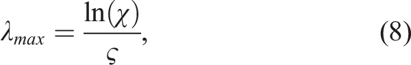
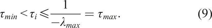
The desired maximum settling time of the closed-loop control is set to ς = 10 s, indicating the maximum time allowed for the system outputs to remain within χ = 5% of their desired values. This value was chosen following the results obtained in Wu (2018) where the proposed nonlinear model-based PID controller designed for the same vehicle and task, displayed an average settling time of 10 s. Therefore, we know that a value ς = 10 is a feasible desired performance for the PID structure. The minimum value of the pole τ _min is determined according to stability and physical requirements. The lower the value of τ _i is, the higher the value of the control parameters becomes. We chose τ _min = 0.5 since, for lower values, the resulting control inputs cannot be physically generated on the real platform (i.e. they exceed the speed controller limits) and they are too aggressive for the control objective. The resulting space of possible pole values is defined as:

${\tau }_i\in [0.5,3.338].$

(10)

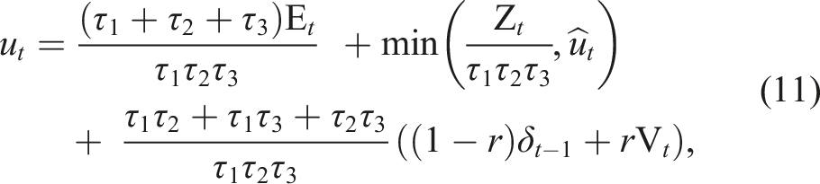
According to the pole-placement design and its resolution proposed in Chaffre et al. (2021), the control input is:

$\begin{array}{cc}\hfill u_t=& \frac{({\tau }_1+{\tau }_2+{\tau }_3){\text{E}}_t}{{\tau }_1{\tau }_2{\tau }_3}+\min (\frac{{\text{Z}}_t}{{\tau }_1{\tau }_2{\tau }_3},{\widehat{u}}_t)\hfill \\ \hfill & +\frac{{\tau }_1{\tau }_2+{\tau }_1{\tau }_3+{\tau }_2{\tau }_3}{{\tau }_1{\tau }_2{\tau }_3}\left((1-r){\delta }_{t-1}+r{\text{V}}_t\right),\hfill \end{array}$

(11)

where τ₁, τ₂ and τ₃ are the poles of the considered feedback loop controller. In scenarios where only limited information about environmental disturbances is available and in the presence of time-varying processes, model-free adaptation can be employed. To account for the uncertainties in pole selection, the proposed approach uses DRL to construct a stochastic predictive model π _μ . This model maps the AUV state vector s _t to the pole values. The learning agent aims to build a predictive model that directly maps the AUV state to the pole values τ _i , which are then used to compute the PID control inputs to regulate the AUV’s position and orientations. This mapping ensures that, for any pole values chosen by the DNN in the parameter cube (Chaffre et al., 2021), the resulting control input will maintain the poles in the left half-plane for the control system only.

4.3. Closed-loop stability discussion

While stability analysis remains a challenging task in control systems with model-free components, it is essential to reduce the risk of instability. One approach is to limit the selection of controllers to those with known stability properties. While this is not a sufficient condition for stability, it is a prudent step in the right direction. Additionally, stability analysis must be performed retrospectively across a range of selected simulations to assess the performance of the chosen controller under various conditions and disturbances. This iterative process can help refine the controller design and ensure stability across different operating scenarios.

We have demonstrated in prior work (Kohler et al., 2022) how Lyapunov stability analysis can be conducted for the proposed learning-based adaptive control design equation (11) in the context of AUVs. We conducted a stability analysis of the learning-based adaptive controller for an AUV using the following Lyapunov function (Kohler et al., 2022):

$V(x)=\frac{1}{2}{x}^T\left[\begin{array}{ccc}\hfill M_{\eta }^{-1}\hfill & \hfill \alpha I\hfill & \hfill 0\hfill \\ \hfill \alpha I\hfill & \hfill k_p\hfill & \hfill k_i\hfill \\ \hfill 0\hfill & \hfill K_i\hfill & \hfill \alpha k_i\hfill \end{array}\right]x,$

(12)

where $\alpha \in \mathbb{R}$ is a small positive constant; $M_{\eta }^{-1}$ is related to the AUV mass and can be computed from the current η; x is the control loop’s state $x={\left[p,\eta ,{\int }_0^{t}e(\tau )d\tau \right]}^T\in {\mathbb{R}}^{18}$ and $p=M_{\eta }{\dot{\eta }}^T\in {\mathbb{R}}^6$ is the generalised momentum, that is dependent on the AUV mass and velocity (Fossen, 2011). The analysis demonstrated that the learning-based adaptive controller displayed similar stability performance as obtained with a Lyapunov-based controller (i.e. a controller which guarantees that V(x) > 0 and $\dot{V}(x)<0$ , ensuring that the vehicle is always converging to globally stable states regardless of the starting state).

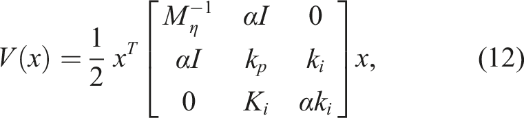
In addition, the Lyapunov function equation (12) has allowed us to identify constraints on the gains k _p , k _i , k _d and the small constant α such that local stability is guaranteed, denoted as control parameters stability. In this case, it was found that the learning-based controller has little to no control parameters stability, meaning that the gains estimated by the ANN did not meet these constraints, despite that the Lyapunov criterion V(x) > 0 and $\dot{V}(x)<0$ are fulfilled.

Another solution for the stability analysis would be to constrain the space of possible value for the poles to solutions that guarantee the Lyapunov criterion. By doing so, we found in Kohler et al. (2022 that the resulting space is so small that the benefits of the learning-based formulation were obliterated. As a result, it is important to note that the proposed learning-based adaptive controller has no proven guarantees that the criterion of the aforementioned Lyapunov function equation (12) are respected. However, in the current study, the evaluation of local stability was not conducted, despite the availability of the Lyapunov function equation (12) and the methodology introduced in our previous work (Kohler et al., 2022). This decision was made due to the absence of rigorous guarantees that could be derived from such an assessment.

5. Model-free adjustment mechanism

5.1. Stochastic policy

To take into account the uncertainties in the pole selection, we propose to use DRL to build a stochastic predictive model π _θ that maps a state vector s _t into the pole values:

$\left\{\begin{array}{cccc}\hfill {\pi }_{\theta }:& S\subset {\mathbb{R}}^{dim(S)}\hfill & \hfill \to & A\subset {\mathbb{R}}^{3\times dim(u)}\hfill \\ \hfill & x={\left[{\mathbf{s}}_t\right]}^T\hfill & \hfill \mapsto & \left[{\lambda }_i,{\mu }_i\right],\hfill \end{array}\right.$

(13)

where $\mathcal{N}({\tau }_i)$ is the probability density function of τ _i that is modelled by a Normal distribution $\mathcal{N}({\tau }_i)$ as:

$\mathcal{N}({\tau }_i)={(2\pi {\mu }_i)}^{-1/2}\exp \left\{-\frac{1}{2{\mu }_i}{(x-{\lambda }_i)}^2\right\},$

(14)

with ${\lambda }_i\in \mathbb{R}$ and ${\mu }_i\in {\mathbb{R}}^{+}$ are the mean and variance of p(τ _i ) that are estimated by the policy network. Therefore, the outputs of the policy network are the 3 × dim(u) pairs of (λ, μ) representing the normal distributions $\mathcal{N}({\tau }_i)$ used to sample the poles for each control input u _i .

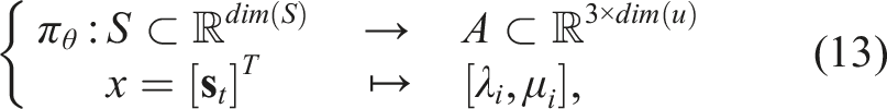
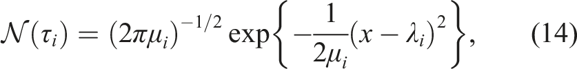
In the literature, the Normal distribution equation (14) is conventionally selected to model actions, ensuring that the estimated actions are centred around the presently estimated optimal action. This choice offers a favourable balance between exploitation and exploration compared to asymmetric distributions like the Pearson distribution. Asymmetric distributions may introduce bias and contribute to the emergence of local minima. The stochastic policy represented in equation (13) prevents early convergence, encourages exploration, and improves the robustness to uncertainties. Moreover, it has been observed that learning a stochastic policy with entropy maximisation drastically stabilises training compared to a deterministic policy (Haarnoja et al., 2018).

In practice, the pole τ _i (t) is sampled from $\mathcal{N}({\tau }_i)$ after applying an invertible squashing function (i.e. tanh) to $\mathcal{N}({\tau }_i)$ (to bound the Gaussian distribution) and after using the change of variable to compute the likelihoods of the bounded action distribution (see Appendix C of Haarnoja et al. (2018) for the complete description of this process). Designing this stochastic function equation (13) is numerically expensive due to the dimensions of the underlying spaces, excluding real-time computation with model-based methods only. The DRL framework allows us to iteratively build an estimate of this optimal mapping function.

5.2. State vector

In this work, at each timestep, the agent captures an observation vector o _t representing the process dynamics which consists solely of variables that are available on the real vehicle. The observation vector is thus defined as:

$o_t=[a_{t-1};X;\mathrm{\Theta };V;\dot{V};\mathrm{\Omega };e_t;e_{L2}],$

(15)

where

• $a_{t-1}\in {\mathbb{R}}^{18}$ are the most recent actions estimated (i.e. poles value),

• X = [x; y; z] are the vehicle position,

• Θ = [ϕ; θ; ψ] are the Euler orientation of the vehicle (roll, pitch, and yaw respectively),

• V = [v _x ; v _y ; v _z ] and Ω = [ω _ϕ ; ω _θ ; ω _ψ ] are respectively the vehicle’s linear and angular velocities,

• $\stackrel{.}{V}=[\dot{v_x};\dot{v_y};\dot{v_z}]$ are the vehicle’s linear acceleration,

• $e_t\in {\mathbb{R}}^6$ are the error values on each setpoint as defined in Section 4,

• and e_L2 is the Euclidean distance to the steady-state defined as $e_{L_2}=\sqrt{{\sum }_{i=1}^{i=dim(u)}{e}_i^2(t)}$ .

The dimension of the observation vector o _t is therefore equal to 40. It is important to note that with this observation vector equation (15) the current disturbance characteristics are not included. To improve the observability of the process and following our previous results (Chaffre et al., 2020), the state vector s _t is obtained out of the current and past observation vectors along with their two-by-two difference. This results in a 120-dimensional state-space defined as:

$s_t=[o_t;o_{t-1};o_{t-1}-o_t]\in {\mathbb{R}}^{120}.$

(16)

DDPG algorithms have shown promise in handling the control tasks of real-world systems (Ye et al., 2021). This architecture simultaneously estimates a value function and a policy function to improve the agent’s performance. Off-policy methods, using Experience Replay (ER), have been developed to enhance the sample efficiency of these functions using past experiences generated by different policies. However, a critical challenge faced by DDPG and TD3 algorithms is the value overestimation problem (Kumar et al., 2019). The value of an action represents the expected cumulative reward that an agent can achieve by taking that action in the current state and following a certain policy. The issue here is that these algorithms can sometimes overestimate the true values of actions, leading to suboptimal decision-making by the agent. Value overestimation can occur when the learning algorithm assigns higher values to actions than they truly deserve. This overestimation can be problematic because it may cause the agent to prefer actions that are not the most optimal in the long run. This issue can impact the overall performance and efficiency of the reinforcement learning algorithm. To mitigate this, this work applies the Maximum Entropy DRL algorithm SAC (Haarnoja et al., 2018) providing a more robust and efficient learning method for DRL-based control systems. The next section introduces the version of SAC used in this work.

5.3. Soft Actor-Critic (SAC) with automatically adjusted temperature

The SAC algorithm (Haarnoja et al., 2018) is a DPG method known for its robustness to uncertainty and its suitability for operating in partially observable processes. SAC combines three key components: improved exploration and stability through entropy maximisation, an actor-critic architecture with separate Q-value and policy networks, and an off-policy formulation using experience replay. Originally, the objective function of SAC is:

$J(\pi |s_0)=\underset{\pi }{\max }{\mathbb{E}}_{\pi }\left[\sum _{t}r(s_t,a_t)+\alpha \mathcal{H}(\pi (\cdot |s_t))|s_0\right].$

(17)

Unlike traditional reinforcement learning algorithms, that optimise the expected sum of rewards, SAC also maximises the entropy $\mathcal{H}(x)={\mathbb{E}}_{x\sim P}[-\log (x)]$ of the behaviour policy weighted by a temperature parameter α (cf. Equation (17)). This promotes exploration and adaptability in the agent’s behaviour, enhancing its resilience to environmental changes. It encourages the agent to investigate less optimal paths until discovering those leading to long-term objectives. The entropy term is explicitly incorporated into the state-value function, which combines Q-value estimates and the policy’s entropy. The temperature parameter α, which controls the stochasticity of the policy, is here controlled indirectly by the reward scale. Unfortunately, it is often difficult to define beforehand an optimal reward scale as the entropy can vary unpredictably both across tasks and during training as the policy becomes better. For this reason, we used an improved version of SAC (Haarnoja et al., 2019) which incorporates optimisation of the temperature term to satisfy a minimum entropy constraint:

$\underset{{\pi }_0,\dots ,{\pi }_T}{\max }\mathbb{E}\left[\sum _{t=0}^{T}r(s_t,a_t)\right]\text{\hspace{0.17em}s.t.\hspace{0.17em}}\forall t\text{,\hspace{0.17em}}\mathcal{H}({\pi }_t)\ge {\mathcal{H}}_0.$

(18)

To reduce value overestimation, this version of SAC (Haarnoja et al., 2019) utilises two Q-value function estimators and applies TD-Learning to iteratively estimate the Q-value functions. The state-value function V(s _t ) is not explicitly represented anymore by a DNN, but it is implicitly defined through the Q-value functions and the policy (as no differences are observed when comparing both methodologies (Haarnoja et al., 2019)). The delayed update technique from the TD3 algorithm (Fujimoto et al., 2018) is utilised. This minimises the chances of repeatedly updating the policy with unchanged information, thereby constraining the variance of the value estimate. The outcome is higher-quality policy updates.

The policy network’s parameters are consequently optimised to minimise the expected Kullback-Leibler divergence between the current policy and the exponential of the Q-value distribution. With this version of SAC, the reward scale does not need to be tuned as the relative weight of the entropy term is adapted to satisfy a minimal entropy constraint. The resulting dual constraint optimisation for the policy can be defined as:

$J(\alpha )={\mathbb{E}}_{s_t\sim D,a_t\sim {\pi }_{\mu }}\left[-\alpha \log {\pi }_{\mu }(a_t|s_t)+\alpha \times 18\right],$

(19)

with $\mathcal{H}=-18=-dim(u)$ is the target entropy, which according to Haarnoja et al. (2019) can be easily set to the negative dimension of the action space. In the present case, the action space has a dimension of 18 since the task is to control a vehicle with 6-DoFs, and each DoF has 3 possible pole values.

5.4. Reward function

Since we are using the second version of SAC (Haarnoja et al., 2019), the reward scale does not require to be tuned. Thus, we proposed the following reward design:

$r(s_t)=\exp \left[-(e_{L2}(t))\right].$

(20)

This reward function is solely a function of the distance to the setpoint included in the state vector in equation (5), which can be maximised if and only if the desired distance equation (3) is minimised. With this second version of the SAC algorithm (Haarnoja et al., 2019), the reward scale does not need to be controlled. Therefore our reward signal equation (20) is defined as r _t ∈ [0, 1] which is more appropriate when using DNNs. In this work, the SAC method summarised above, was extended with the Biologically Inspired Experience Replay (BIER) method (Chaffre et al., 2022b) introduced next.

5.5. Biologically Inspired Experience Replay (BIER)

The BIER method (Chaffre et al., 2022b) aims to combine the resilience of the on-policy sampling with the data efficiency of off-policy formulation and, in general terms, it is defined by two distinct memory units: the sequential-partial memory (B1) and the optimistic memory (B2).

The B1 memory unit serves a purpose similar to the memory buffer in the original definition of Experience Replay (ER). In the context of robotics, where optimal behaviour is often highly temporally correlated, learning a limited set of such sequences can efficiently lead to optimal behaviour. However, using temporally correlated samples can compromise learning in DNNs of the underlying SAC method due to overfitting and lack of Independence and Identical Distribution (I.I.D.) in the training dataset. To address this issue, BIER incorporates the concept of partial transitions in B1, whereby only one out of every two transitions is added to this buffer. This approach adds a regularisation effect to the DNN fitting process, reducing the age of the oldest policy stored in B1, thereby improving the learning performance (Fedus et al., 2020).

The B2 memory unit represents an optimistic memory and is inspired by the observation that positive reinforcement is more efficient in biological systems than a combination of positive and negative rewards. B2 stores the upper outliers of the reward distribution, which are considered to be the best transitions. By increasing the probability of using past transitions associated with high-quality regions in the solution space, B2 aims to enhance performance improvement (Fedus et al., 2020).

Finally, BIER consists of randomly sampling n temporally correlated sequences from B1 (i.e. a temporal sequence composed of n consecutive transitions) and randomly sampling n uncorrelated transitions from B2 to construct the mini-batch of past experience to perform the mini-batch gradient descent optimisation procedure of the DNNs.

5.6. Domain randomisation

Despite the stability components of our learning-based adaptive controller described in Chaffre et al. (2021), training directly on the real platform is not a possibility due to the vehicle’s limited battery life, added to the time to run the number of trials needed to train the RL agent. Therefore, in this work, training was performed on a simulated version of the BlueROV platform, and the learnt policy was transferred to the physical platform. In this case, the distribution shift arises from the transfer of a policy trained in a near-perfect state-space (obtained in a simulated environment) to an agent subject to sensor noise, delays, and a real turbulent environment.

Various techniques exist to reduce the reality gap between simulation and the real world, such as Domain Randomisation (DR) (Tobin et al., 2017). In DR, the environment used for training is referred to as the source domain, while the environment we aim to transfer to is denoted as the target domain. Typically, training is only feasible within the source domain, where a set of N randomisation parameters can be modulated to alter the domain’s characteristics. Thus, a configuration ξ can be defined as a sample drawn from a randomisation space $\xi \in \mathrm{\Xi }\subset {\mathbb{R}}^N$ . During training, the data from the source domain are collected with the application of randomisation to the parameters. By doing so, the policy is exposed to a diverse range of distinct versions of the source environment, allowing for a better generalisation to be learnt compared to exposure to a single environment. The appearance of the environment can be controlled by the following randomisation parameters: position, shape, and colours of the objects; the texture of material; lighting condition; random noise added to images; or position, orientation, and field of view (FoV) of the simulated camera. These parameters can also control the physical dynamics of the domain such as the mass and dimension of objects, the mass and dimension of vehicles, damping and friction of the joints, observation noise, or action delay.

The idea of incremental environment complexity (Chaffre et al., 2020) was employed in this study as a modification of the DR procedure. The approach involved training the agent in diverse variations of the same environment, each differing in task complexity as indicated by the quantity and shape of obstacles present. The agent would transition between these domains based on its performance, as assessed by the success rate. This method offers the advantage of preventing the agent from becoming trapped in an unfavourable regime by returning it to a previously solved complexity level if it fails to solve the current one. By appropriately adjusting the parameters, a smooth transition can be ensured as the agent progresses through each configuration until reaching the final one. However, it is important to note that this approach lacks control over the amount of data collected from each complexity configuration. Consequently, some configurations may be extensively explored while others receive less attention, potentially leading to overfitting. We can mitigate this issue by forcing the agent to collect the same amount of data from each complexity configuration, from the simplest to the more challenging one (Chaffre et al., 2022a). Nevertheless, it is difficult to determine beforehand the appropriate amount of data that the agent will require to solve a configuration. With this approach, additional tuning of this parameter is necessary to ensure that no time is wasted on already solved configurations and that enough time is provided on the difficult ones.

Due to these considerations, this study examined three environment configurations characterised by varying levels of complexity, assessed based on the degree of disturbance:

• Configuration 1: no disturbance at all.

• Configuration 2: current disturbance that does not vary within the episode.

• Configuration 3: current disturbance that changes at a random time within the episode between timestep 100 and 400, out of 500. The value 500 was chosen as the maximum value for the length of the episodes following the desired settling time defined in Section 8.

At the outset of each episode, the agent is equally likely to encounter any of the previously described environment configurations. This approach ensures a uniform exploration of each configuration, preventing overfitting. Additionally, it facilitates early exposure to the most challenging environment configuration, which closely resembles the target domain, thereby enhancing sample efficiency during the training phase. This methodology is illustrated in Figure 2 where the choice of complexity configuration is performed after the end of each episode.

Figure 2.

Illustration of the domain randomisation technique. During training, the agent experiences a large number of variations of 3 environment configurations. Each configuration has the same probability p = 1/3 to be chosen.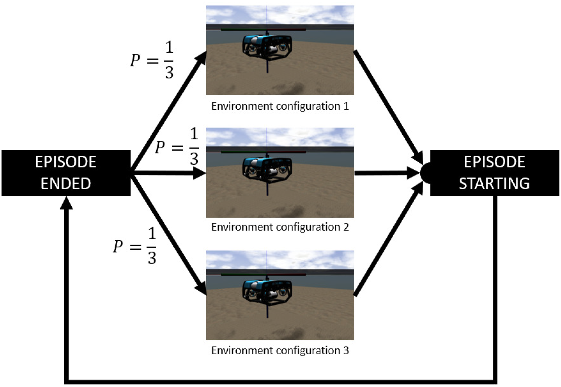

5.7. Exploration strategy

We used adaptive parameter noise (Plappert et al., 2018) where random Gaussian noise $\mathcal{N}(0,\sigma )$ is added to the parameters of the policy network (weights and bias) at the beginning of each episode (then kept during the rollout) as:

${\sigma }_{k+1}=\left\{\begin{array}{c}\alpha {\sigma }_k,\mathbf{i}\mathbf{f}d(\pi ,\tilde{\pi })<\delta ,\hfill \\ \frac{1}{\alpha }{\sigma }_k,\mathbf{o}\mathbf{t}\mathbf{h}\mathbf{e}\mathbf{r}\mathbf{w}\mathbf{i}\mathbf{s}\mathbf{e}.\hfill \end{array}\right.$

(21)

The noise standard deviation σ is adapted according to a distance measure d(⋅) between the non-perturbed π and perturbed policy $\tilde{\pi }$ defined in Plappert et al. (2018) as:

$d(\pi ,\tilde{\pi })=\sqrt{\frac{1}{N}\sum _{i=1}^N{\mathbb{E}}_s[{(\tilde{\pi }{(s)}_i-\pi {(s)}_i)}^2]},$

(22)

where the metric ${\mathbb{E}}_s[\cdot ]$ is estimated over a batch of 1000 samples from the replay buffer, the initial standard deviation is set to 1.0, the threshold is set to 0.10 and the update rate is set to α = 1.005. This strategy can be seen as a middle ground between evolution strategies and DRL. As recommended by the authors (Plappert et al., 2018), to avoid local maxima, which can still happen with a perturbed and stochastic policy, the parameter noise was combined with an ϵ-greedy policy where each action holds an independent probability ϵ = 0.01 to be random.

6. Learning-based adaptive pole-placement

Figure 3 summarises the overall learning-based adaptive control methodology proposed in this paper. We designed an adaptive pole-placement control structure where the gains of the PID law are transformed into the poles domain to be placed in appropriate locations by a DRL-based policy, before being transformed back into the temporal domain to compute the associated PID control input. The pole values are estimated by a policy represented by a DNN whose parameters are optimised using a DPG method. In our case, we used the second version of the SAC algorithm (Haarnoja et al., 2019) to learn the optimal policy for the considered reward function equation (20). The policy, along with the value functions, is learnt offline with TD-Learning (Sutton and Barto, 2018) using the BIER method (Chaffre et al., 2022b) for improved sample efficiency and by using the improved domain randomisation methodology defined in Section 5. After training, the resulting policy is directly transferred to the real platform. In practice, the control parameters constantly vary during the AUV operation to cope with current disturbance variations. As previously discussed, different operating conditions will require different control parameters to minimise the tracking error. Therefore, the objective of the method is to learn the best set of control parameters for every operating condition possible by exploiting the BIER method and then to facilitate the transfer of that knowledge to the physical vehicle via enhanced Domain Randomisation.

Figure 3.

Diagram representing the proposed overall learning-based adaptive control system.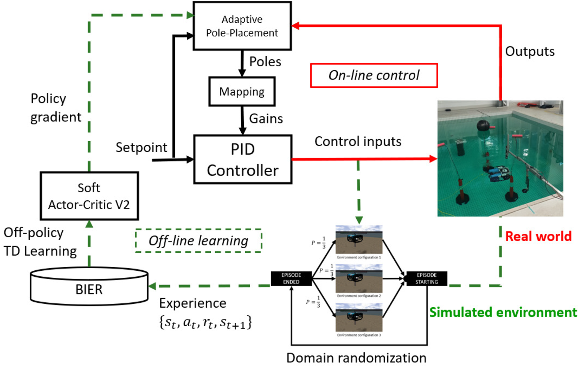

7. Simulated training

The simulation environment was based on the Gazebo robotics simulator and used the UUV Simulator package (Manhães et al., 2016). This combination provided several modules implementing a variety of maritime systems including a range of maritime sensors and systems. The vehicle hydrodynamic model was based on the work of Wu (2018) who developed a model of the vehicle based on a combination of theoretical work and data published by Sandøy (2016).

The simulation was then configured using the mass, added mass, linear and quadratic drag terms derived from Wu (2018). The added mass refers to the increase in inertia experienced by the AUV as it displaces water in its surroundings during movement. This addition of mass contributes to a more realistic simulation of the ROV’s dynamics. The thrusters of the AUV were incorporated using the straightforward first-order thruster model sourced from the UUV Simulator. These thrusters were positioned on the model in accordance with the orientations and moments estimated by Wu (2018). The desired force and torque of the simulated vehicle were set by a ROS topic, and individual thruster effort was allocated using the Thruster Allocation Matrix (TAM) provided by the simulator. The vehicle’s pose and velocity estimates were published as a single odometry message on another ROS topic. Using these topics, a MIMO control system was used to guide the vehicle to perform station keeping.

A simulated training episode was defined as follows:

(1) At the beginning of the episode the AUV was initialised at the position (x₀, y₀) ∈ [−5, 5], z₀ ∈ [−20, − 10] with null velocity and a random orientation (ψ₀, θ₀, ϕ₀) ∈ [−π/4; π/4].

(2) A random configuration of the environment was generated as defined in Section 5.

(3) A random setpoint was generated with coordinates defined as (x _w , y _w ) ∈ [−5, 5], z _w ∈ [−15, − 5], (ψ _w , θ _w ) = 0, and ϕ _w ∈ [−π/2, π/2].

(4) Then, the off-policy exploration strategy was used and the episode ended when the step number reached 500.

This task aims to train the agent to effectively maintain its position (station keeping) under diverse conditions. The evaluation scenario involves a sequence of training episodes with varying setpoints, challenging the agent to adapt and perform station keeping effectively in different situations. The training consisted of performing a total of 5000 episodes of maximum timesteps set to 500 which took approximately 4 h (considering that the training was conducted using a ‘real-time factor’, this implies that it is equivalent to 4 hours of actual vehicle usage in real-life conditions). Before an episode begins, the configuration of the environment characteristics was chosen as described in Section 5.

The complete list of hyperparameters is provided in Table 1 with the details on the DRL framework.

Table 1.

List of hyperparameters and their values for the simulated training.

Training hyperparameter	Value
Number of hidden layers (all networks)	2
Number of hidden nodes (all networks)	256
Mini-batch size	256
Activation function	Leaky ReLU
Optimiser (all networks)	Adam
Learning rate (all networks)	0.0003
Discount factor (γ)	0.99
Target network smoothing coefficient (Δ)	0.005
Critics L2 regularisation	0.001
Target entropy	−18
Replay buffer max size	1,000,000
Replay start size	10,000
Experience replay method	BIER
Delayed update trick (Fujimoto et al., 2018)	True
Layer normalisation (Ba et al., 2016)	True
Automatic temperature adjustment	True

The training curves are presented in Figure 4. The performance of the proposed learning-based controller is depicted in red (with the shaded regions representing the standard deviation) and the performance of its model-based counterpart is represented in blue. The model-based controller is the controller proposed in Wu (2018) described in Section 3. The training performances are the mean values of the aforementioned metrics computed over 100 random evaluation episodes that are computed every 100 episodes. The performance of the model-based controller (in blue in Figure 4) has been averaged over 1000 random episodes. As we can see in the top plot of Figure 4, the learning-based controller was able to learn the task and converge toward the maximum reward value. In the second plot of Figure 4, the control performance is displayed in terms of RMSE on the setpoint. We can see that the learning-based adaptive controller outperformed the control performance of the model-based controller, which is represented by the blue horizontal lines. In the next section, the experimental evaluation of the resulting policy is presented.

Figure 4.

Training curves of SAC with learnt temperature. This process corresponds to simulated pre-training on 2.5 million samples, taking around 4 h.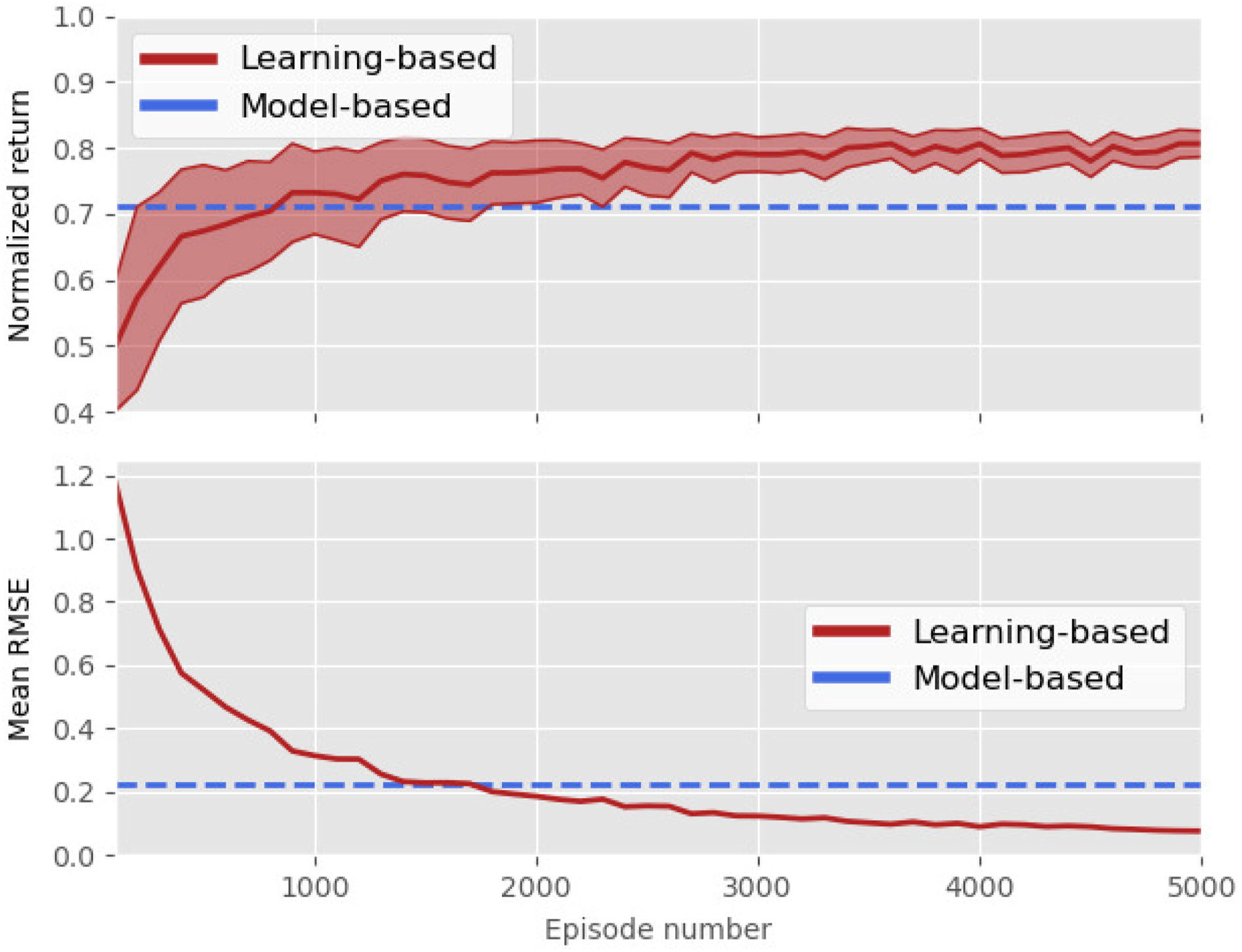

8. Experimental setup

This section presents the results of the experimental evaluation campaign where the policy trained under simulation is transferred to a real vehicle in the environment depicted in Figure 1. This campaign covered approximately 280 min (or ∼4h40) of real-life operating time.

8.1. Physical vehicle

For the effective sim-to-real transfer, the physical vehicle should match the interface of the simulation. To meet this requirement, the system shown in Figure 5 was defined. It uses an Ethernet-based network, allowing the transfer of pose and control information between shore systems, while a pair of Blue Robotics Fathom-X boards allows Ethernet communication with the AUV across a tether. With this network, high-speed low-latency communication can be performed between the shore systems and the AUVs onboard computer systems. Combined with the ROS’ ability to operate in a network transparent manner, robotics software can be distributed across multiple systems while performing effective estimation and control of the AUV.

Figure 5.

Physical block diagram of the experimental setup. This diagram includes both the BlueROV 2 Heavy and the shore equipment used for monitoring and control.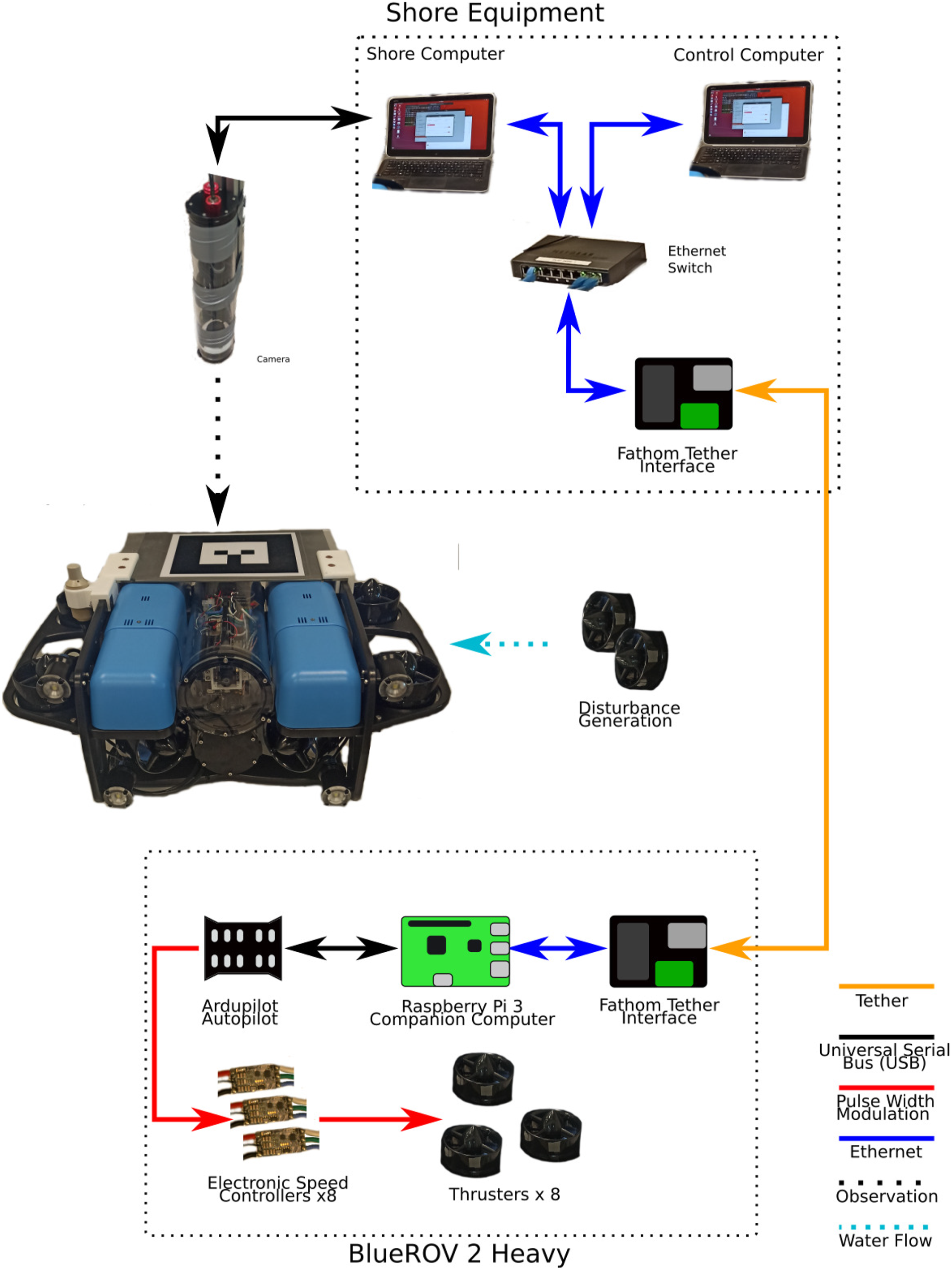

The onboard processing on the AUV was provided by a Raspberry Pi 3 single-board companion computer. This system ran an Ubuntu-based system with a ROS Kinetic package developed by Blue Robotics (Blue Robotics Inc., 2015). This computer communicated with a Pixhawk autopilot (PX4 Dev Team, 2019) running the Ardupilot firmware via the Micro Aero Vehicle Link (MAVLink) protocol. This allowed the control and monitoring of the vehicle using QGroundcontrol, a standard base station for drone vehicles (QGroundControl, 2019). This data was also communicated to the ROS system using an instance of the MAVROS MAVLink to ROS gateway (Ermakov, 2019).

The BlueROV’s PixHawk autopilot contains sensors capable of estimating attitude and orientation information but it is not capable of producing an absolute position estimate. Therefore, this work used a hybrid localisation system, with an external camera and a marker placed on the top side of the vehicle.

The camera was mounted within a Blue Robotics waterproof enclosure with its optical centre in a transparent dome. The camera assembly was attached to an aluminium frame such that the end of the enclosure was beneath the water level, and facing downward as illustrated in Figure 1(a). This gave a clear view of the BlueROV while minimising distortion due to refraction. With the assembly mounted in the immersion tank, the camera was calibrated using a waterproof checkerboard.

In this configuration, the camera system had a clear view of the vehicle, allowing visual tracking to be performed. The marker pose was estimated using the ar_track_alvar ROS package (Niekum and Saito, 2019) which uses the ALVAR library (VTT Technical Research Centre of Finland Ltd, 2019) to track fiducial markers. The recovered pose of the marker was fused with data from the autopilot using the robot_localization package (Moore and Stouch, 2016). This solution allowed a bounded estimate of vehicle pose and velocity information which was published as a ROS odometry message of the same type as published by the simulator.

The control of the vehicle was done via a ROS Wrench message, containing both force and torque terms. This information was mapped via a custom node into a joystick override message. Estimation of the thruster effect is a challenging task, with the force generated by a thruster varying significantly based on factors such as the speed of the propeller, and the rate of advance of the vehicle.

For this project, the thruster effect was estimated from the force curves published by Blue Robotics (Blue Robotics Inc, 2017b). These are static thrust curves generated by bollard pull tests within a static environment. Using these thrust curves, the thruster forces were linearised around the expected operating point of 1400-1600 microseconds, corresponding to a force of +/− 5 N. This was then used to generate the coefficients shown in Table 2. This mapping was used to convert between the desired force on the vehicle and the control values passed to the autopilot.

Table 2.

Wrench to joystick override mappings.

Mapping	Calculation	Coefficient
Thruster force	25/(0.2 ∗ 9.8)	12.8
Roll torque	thrusterforce/(0.218 ∗ 4)	14.7
Pitch torque	thrusterforce/(0.12 ∗ 4)	26.7
Yaw torque	thrusterforce/(0.1888 ∗ 4)	17.0

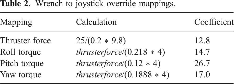
Once in a suitable format, the message was sent to the autopilot via the MAVROS node. The autopilot used the override signal with a TAM matrix to allocate effort to the vehicle’s brushless Electronic Speed Controllers (ESCs), which in turn drove the T200 thrusters that move the vehicle.

Using this configuration, the control system was tested on a real-world underwater vehicle using the same topics and message types as the simulated vehicle. Next, further details on the positioning system are provided.

8.2. Positioning system

As introduced above, a positioning system was utilised to provide a continuous and accurate estimate of the AUV’s pose and velocities in 6DOF as detailed in equation (1). This estimate was generated by fusing the available measurements utilising an Extended Kalman Filter (EKF). Measurements in the configuration utilised in this experiment included acceleration and rotational rate from the IMU on the Pixhawk, depth from the BlueROVs pressure sensor, and pose from a tag tracking system utilising a webcam. The tracking system applied was the ar_track_alvar ROS package (Niekum and Saito, 2019) which uses the ALVAR library (VTT Technical Research Centre of Finland Ltd, 2019) to track fiducial markers in this experiment using a Microsoft Lifecam configured to the resolution of 720 × 1280 at a rate of 30 Hz in a waterproof housing. To consider the optical characteristics of water, the intrinsic parameters of the web camera were calibrated under the specific configuration intended for the experiment. This calibration took place underwater, at distances expected during the experiment and within the range where effective object tracking is feasible.

The fiducial marker was made as large as possible to maximise the range at which tracking could occur but was within the limits of the ROV. The tag was manufactured from laser-cut acrylic and treated to make the surface matte to prevent reflections. This resulted in a system which could track the marker at a distance between 0.5 m and 2.5 m of the camera. Due to the limitations in the camera’s lens calibration, the tracking was optimally calibrated for a distance of 1.5 to 2.5 m. The limitations in calibration in combination with the FOV of the camera and lens properties an optimal operating region was calculated, as illustrated in Figure 6.

Figure 6.

Operational region of AR tracking system due to limitations in the camera lens calibration FoV and tracking.

The measurements generated by the tracking system were transformed from the frame of reference of the camera to the frame of reference of the BlueROV making it suitable for integration in the state estimation. These measurements were fused using an EKF implemented in the robot_localization package (Moore and Stouch, 2016). To maximise the responsiveness of the estimate, the update rate of the implemented EKF was set to 50 Hz to match the data rate of the IMU, the fastest sensor. The specific configuration of the measurements is presented in Table 3 detailing the mapping between the sensors and the estimated state. The measurements of z, ϕ, and θ provided by the tag tracker were set differential, that is, difference in the available measurements to generate rate measurements, to avoid inconsistencies, and biases, between these measurements and the more accurate measurements from the accelerometer and depth sensors for these states.

Using the above configuration, beyond the otherwise default configuration, the robot_localisation package produced stable estimates, with approximate confidence bounds of +/− 5 mm. Notable divergences from this behaviour occurred in scenarios corresponding to limits in the camera lens calibration and tracking system.

Table 3.

Mapping of measurements to EKF.

Sensor	Rate (Hz)	State	Mapping
Accelerometer	50	ϕ	Absolute
		θ	Absolute
Gyroscope		ω ψ	Absolute
		ω θ	Absolute
		ω ϕ	Absolute
Pressure	10	z	Absolute
Tag	30	x	Absolute
		y	Absolute
		z	Differential
		ϕ	Differential
		θ	Differential
		ψ	Absolute

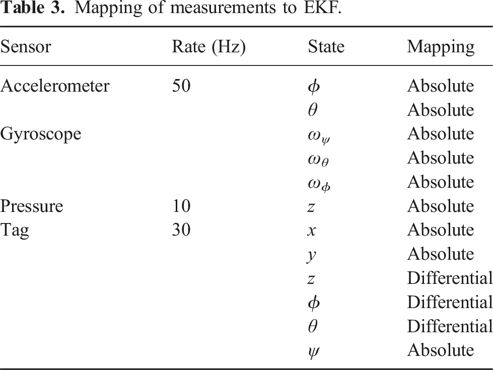
When the depth of the AUV exceeded 2.5 m, or when the tag went out of field view, tracking became inconsistent affecting the accuracy of the estimate. The position and orientation estimate are illustrated in Figure 7 by the RVIZ marker on the right of the screen.

Figure 7.

Illustration of the camera feedback (left of the screen) and the EKF pose estimate represented by the position vectors (right of the screen).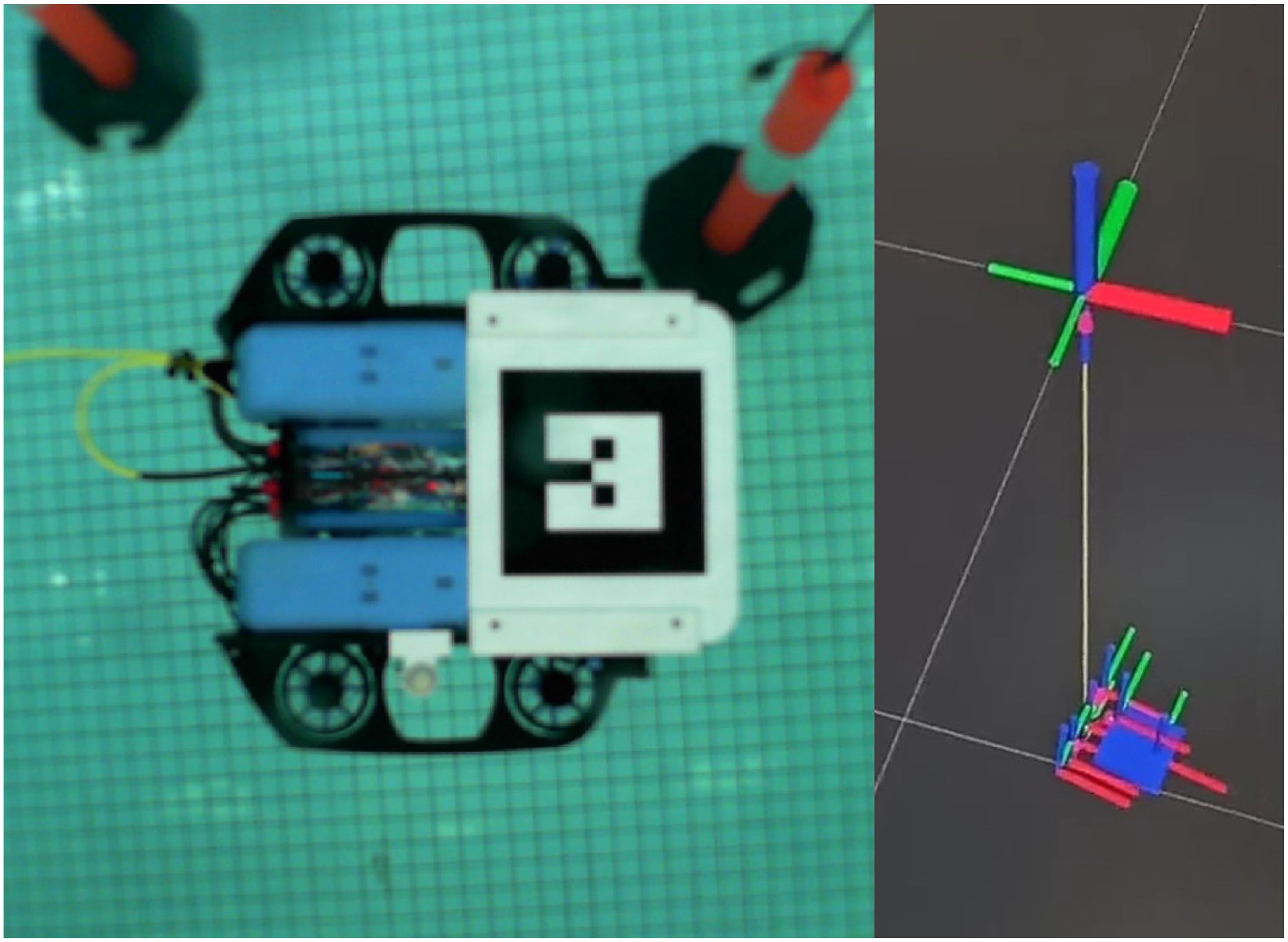

8.3. Disturbance generator

To evaluate the robustness of the controllers against disturbance, we proposed to create an artificial current in the water tank. To that end, we fixed two thrusters of type T200 (the same as the ones on the BlueROV platform) on the aluminium arm where the camera is attached as illustrated in Figure 8. We chose a particular placement and orientation of the thruster such as to optimise the field of effect in the pool. The thrusters are controlled through ESC input that we set to 1625, which according to Blue Robotics documentation gives around 8 N of thrust per thruster. The total current draw for the pair is approximately 2.7 A, providing a power draw of around 38 W.

Figure 8.

Illustration of the disturbance generator system (a) and the marker tracking system (b).

8.4. Task execution

For the physical robot, the multi-station keeping control was executed as follows: starting from an initial position, the vehicle was required to perform station keeping for an amount of 1000 timesteps (∼45 s) at each setpoint, as shown in Figure 9. Each session was, therefore, equivalent to $\sim 7$ minutes. Both controllers were evaluated under two environmental conditions: with and without current disturbance. Each station keeping experiment was conducted 10 times by the physical robot for every control method examined in this study and for each disturbance configuration. The reported results correspond to the average values obtained from these 10 trials.

Figure 9.

Top view illustration of the multi-station keeping task performed during the experimental evaluation.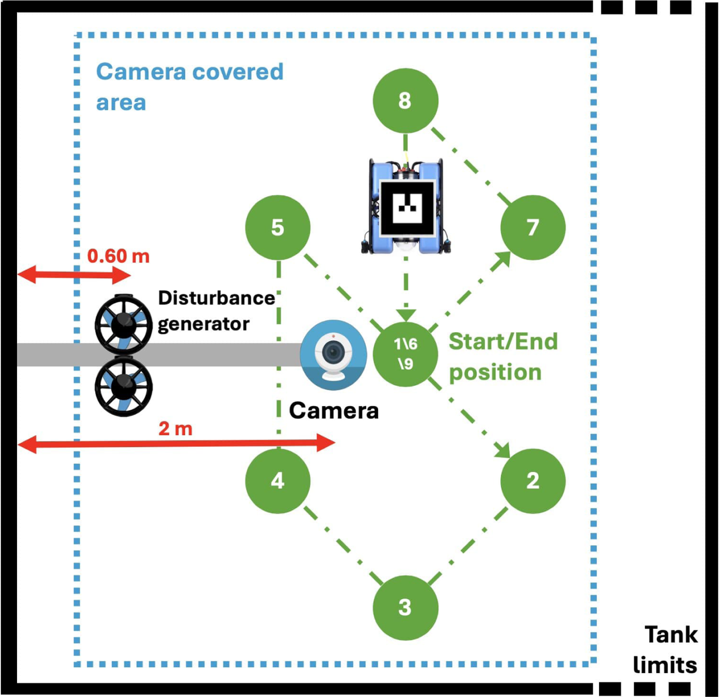

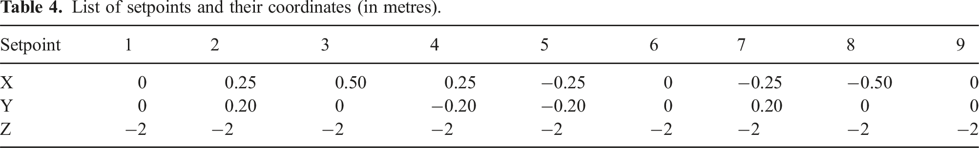
To mitigate potential bias in this evaluation, an initialisation procedure was executed wherein the vehicle is initially brought to the first setpoint. This involves activating the control system when the vehicle is near the setpoint, allowing the control system to stabilise the vehicle over a fixed number of timesteps matching the duration of the subsequent experiments (i.e. 1000 timesteps). Subsequently, the experimental session commences from this same setpoint. In practice, it means that there is an additional setpoint 1 in the list presented in Table 4, which is not taken into account when calculating the performance metrics. This guarantees that the AUV always starts around the same position. We found this practice to be particularly relevant when current disturbances were present since, without the additional setpoint, the starting point of the sessions was distinct due to the current-generated drift.

Table 4.

List of setpoints and their coordinates (in metres).

Setpoint	1	2	3	4	5	6	7	8	9
X	0	0.25	0.50	0.25	−0.25	0	−0.25	−0.50	0
Y	0	0.20	0	−0.20	−0.20	0	0.20	0	0
Z	−2	−2	−2	−2	−2	−2	−2	−2	−2

The experimental task is illustrated in Figure 9 showing the 9 setpoints considered. The disturbance generator and the camera were fixed to an aluminium arm that is fixed on the side of the pool at respectively 60 cm and 2 m from the edge. The vehicle was set to perform station keeping at each setpoint following their numerical order.

9. Experimental results

9.1. Without current disturbance

This section presents the results of the experiments described earlier. The results shown in Tables 5–8 are associated with the experimental scenario in which no current disturbance was applied to the vehicle. We compare the proposed learning-based (LB) controller to the model-based (MB) controller using the following metrics: the root mean squared error (RMSE) on the setpoint to represent the tracking performance, the standard deviation of the RMSE to depict the smoothness of the control, the norm of the control input for power consumption, and the normalised mean return as a proxy for the sim-to-real transfer performance.

Table 5.

Mean RMSE without disturbance.

Setpoint	Model-based	Learning-based
1	0.1189	0.0414
2	0.1366	0.0509
3	0.1673	0.0546
4	0.1433	0.0544
5	0.1085	0.0740
6	0.0914	0.0498
7	0.1380	0.0534
8	0.1311	0.0463
9	0.1106	0.0622

Table 6.

Std RMSE without disturbance.

Setpoint	Model-based	Learning-based
1	0.0241	0.0147
2	0.0325	0.0229
3	0.0335	0.0242
4	0.0332	0.0254
5	0.0376	0.0295
6	0.0247	0.0216
7	0.0355	0.0237
8	0.0471	0.0256
9	0.0520	0.0285

Table 7.

Normalised mean ∑|u| without disturbance.

Setpoint	Model-based	Learning-based
1	0.1365	0.1361
2	0.1575	0.1507
3	0.1806	0.1464
4	0.1907	0.1494
5	0.1036	0.1528
6	0.0880	0.1526
7	0.1209	0.1428
8	0.1141	0.1408
9	0.1289	0.1579

Table 8.

Normalised mean return without disturbance.

Setpoint	Model-based	Learning-based
1	0.7698	0.8992
2	0.7517	0.8815
3	0.6934	0.8740
4	0.7185	0.8738
5	0.7871	0.8390
6	0.8336	0.8863
7	0.7353	0.8769
8	0.7617	0.8929
9	0.7785	0.8595

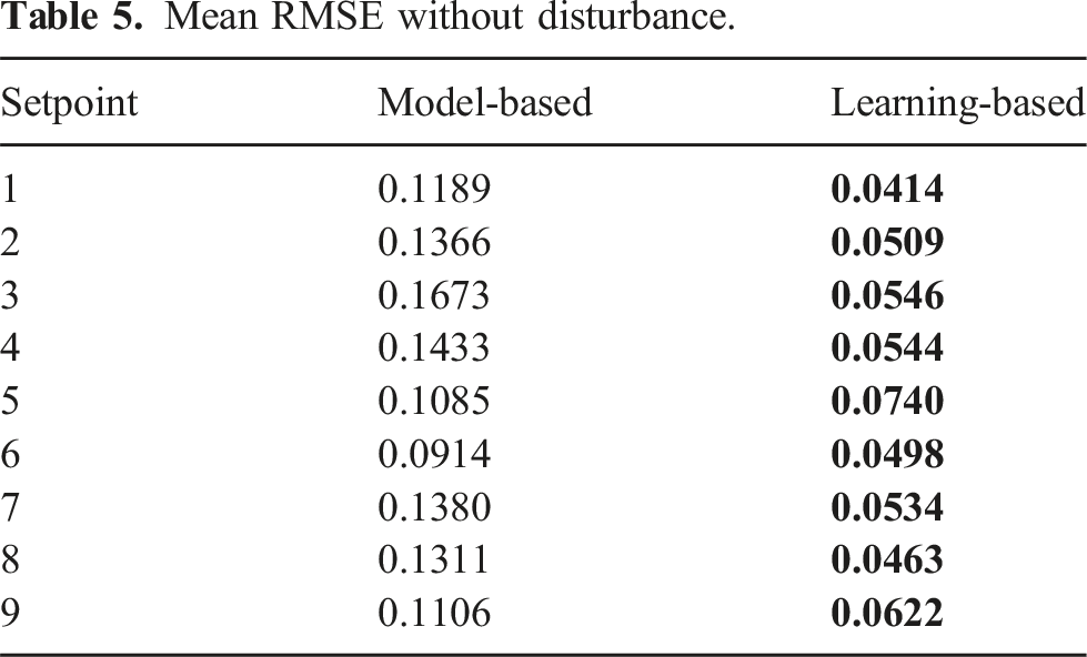
In terms of root mean squared error (RMSE) on the setpoint (see Table 5 above), the LB controller holds the smallest RMSE for every setpoint. On average, the RMSE without disturbance is 2.35 times smaller with our LB controller.

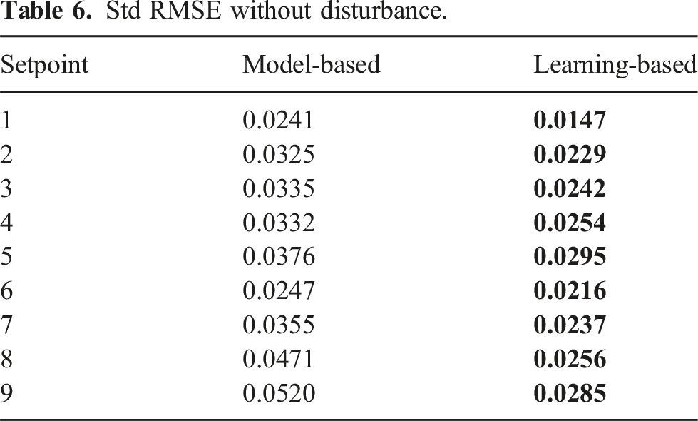
When we take a look at the standard deviation (Std) of the RMSE (see Table 6 above), which can be seen as a measure of robustness, we can also observe that the LB controller is doing better than the MB controller on every setpoint. The Std of the RMSE is again on average about 2 times smaller with our method. This tendency is furthermore perceptible in the violin plots provided in Figure 10 where we can see the median and quartile values computed over the 10 trials. On average, the Std of the RMSE without disturbance is 1.48 times smaller with our LB controller.

Figure 10.

Illustration of the experimental performance of the controllers without disturbance.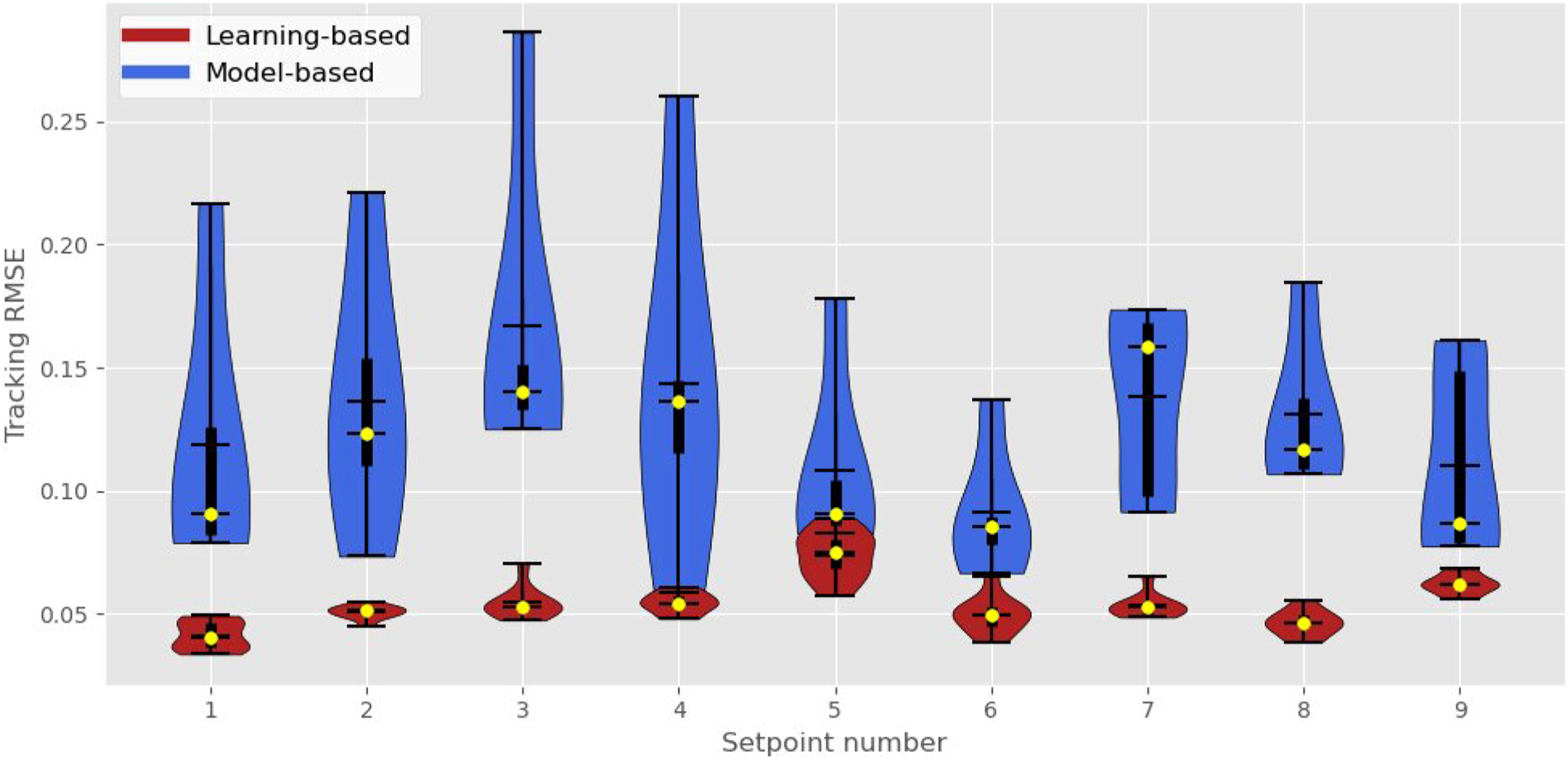

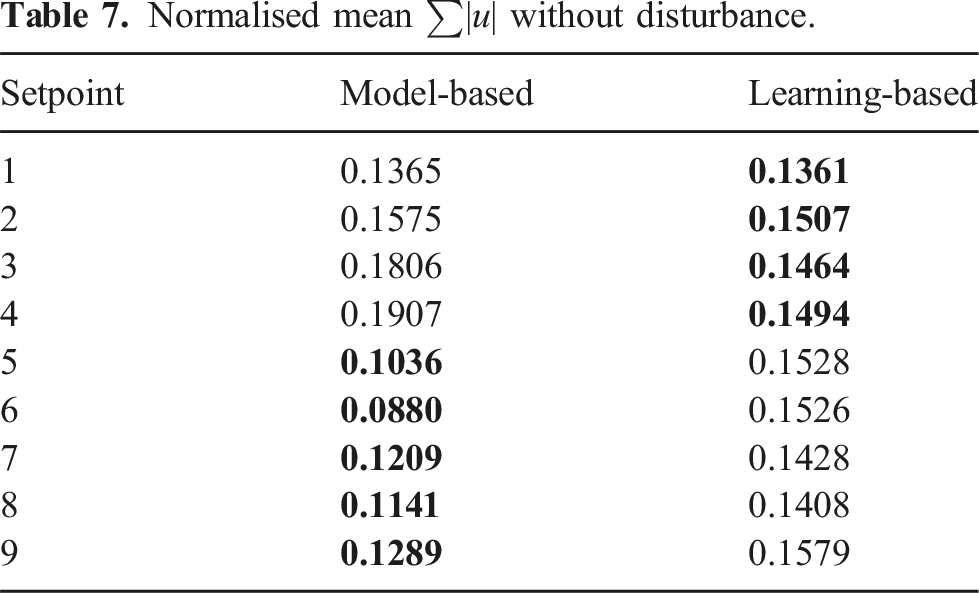
When we take a look at the norm of the control inputs (see Table 7 above), which can be seen as a measure of power consumption, we can observe a less apparent difference between the models. For the first four setpoints visited, the LB controller required smaller values of control inputs to stabilise the vehicle, while it required larger control inputs to stabilise the vehicle at the last five of the visited setpoints. On average, without disturbance, the LB controller consumed 15% more energy than the MB controller.

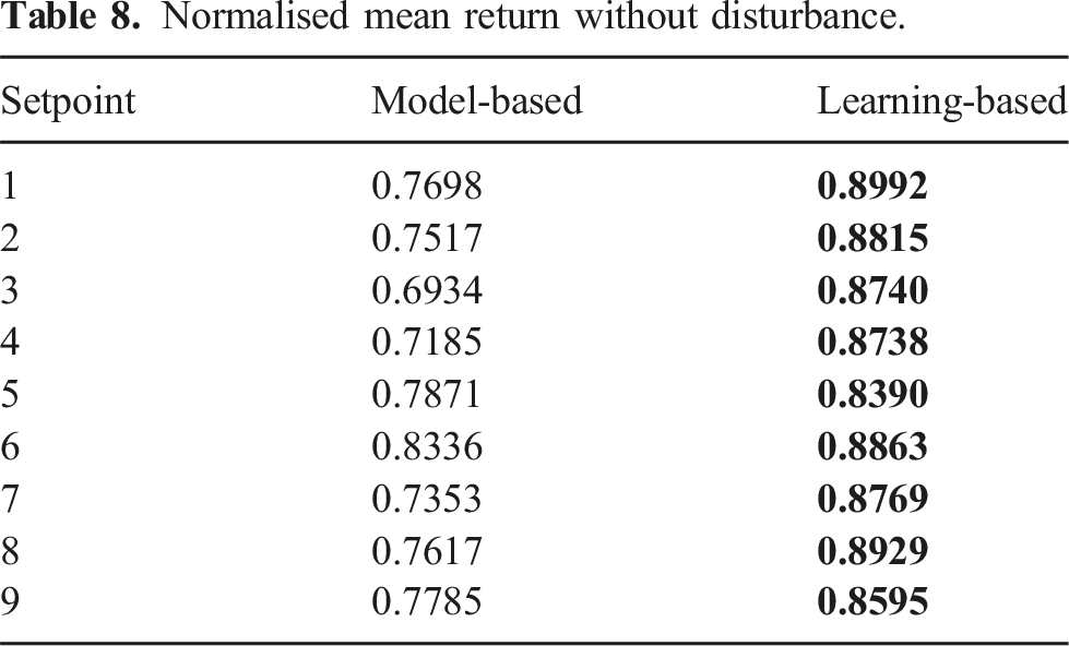
Finally, when we take a look at the mean total reward generated per episode by the agents (see Table 8 above), which can be used as a metric to assess if the policy is behaving as desired, we can see that our LB controller had superior performance at every setpoint. On average, without disturbance, the gain in normalised mean return is about 15% with our LB controller. In Figure 10, we can see that the performance of the LB controller is better (i.e. lower error) and more robust than the MB controller (i.e. less disseminated).

9.2. With current disturbance

When facing current disturbances, the benefits of the proposed method are even more prominent. This is illustrated in the results provided in Tables 9–12 that are associated with the experimental scenario where a current disturbance was applied to the vehicle. Again, we can see that the LB controller presented a better performance compared to the MB controller. In terms of RMSE on the setpoint (see Table 9 below), the LB controller obtained the smallest RMSE for every setpoint. On average, the mean RMSE against disturbance is 3.72 times smaller with our LB controller.

Table 9.

Mean RMSE with disturbance.

Setpoint	Model-based	Learning-based
1	0.3723	0.0882
2	0.3587	0.0844
3	0.3420	0.0731
4	0.3645	0.0783
5	0.3686	0.1120
6	0.3647	0.0797
7	0.3648	0.1149
8	0.3606	0.1385
9	0.3826	0.1100

Table 10.

Std RMSE with disturbance.

Setpoint	Model-based	Learning-based
1	0.1573	0.0289
2	0.0947	0.0330
3	0.0888	0.0285
4	0.1068	0.0294
5	0.0893	0.0451
6	0.1005	0.0277
7	0.0969	0.0319
8	0.0987	0.0530
9	0.1206	0.0444

Table 11.

Normalised mean ∑|u| with disturbance.

Setpoint	Model-based	Learning-based
1	0.1449	0.1816
2	0.1407	0.1739
3	0.1362	0.1407
4	0.1406	0.1475
5	0.1424	0.1637
6	0.1417	0.1311
7	0.1404	0.1389
8	0.1424	0.1874
9	0.1530	0.1717

Table 12.

Normalised mean return with disturbance.

Setpoint	Model-based	Learning-based
1	0.5260	0.7972
2	0.6642	0.8008
3	0.6648	0.8384
4	0.6309	0.8348
5	0.5326	0.7753
6	0.5646	0.8309
7	0.5461	0.7752
8	0.6478	0.7486
9	0.4831	0.7840

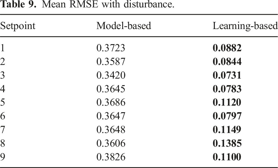
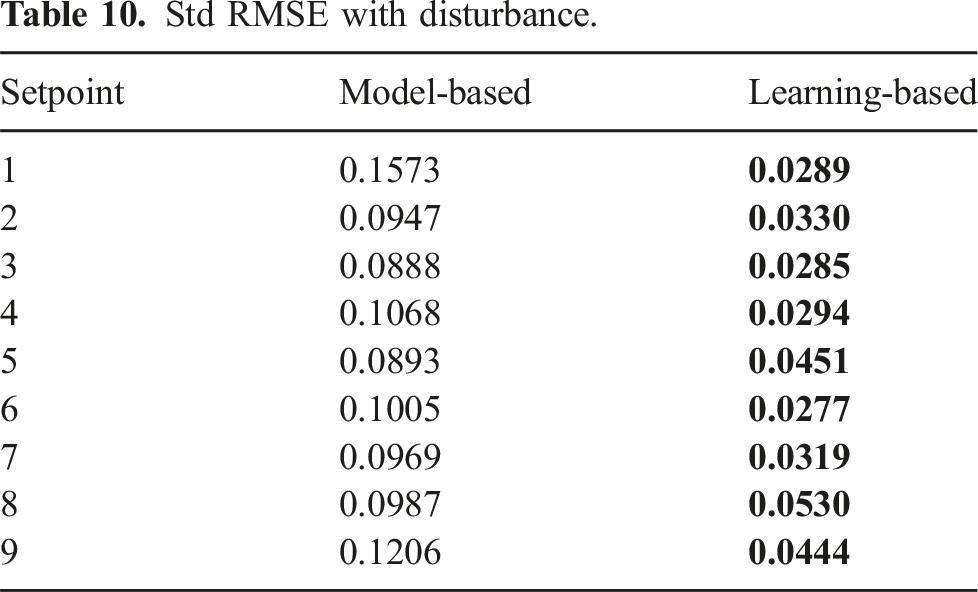
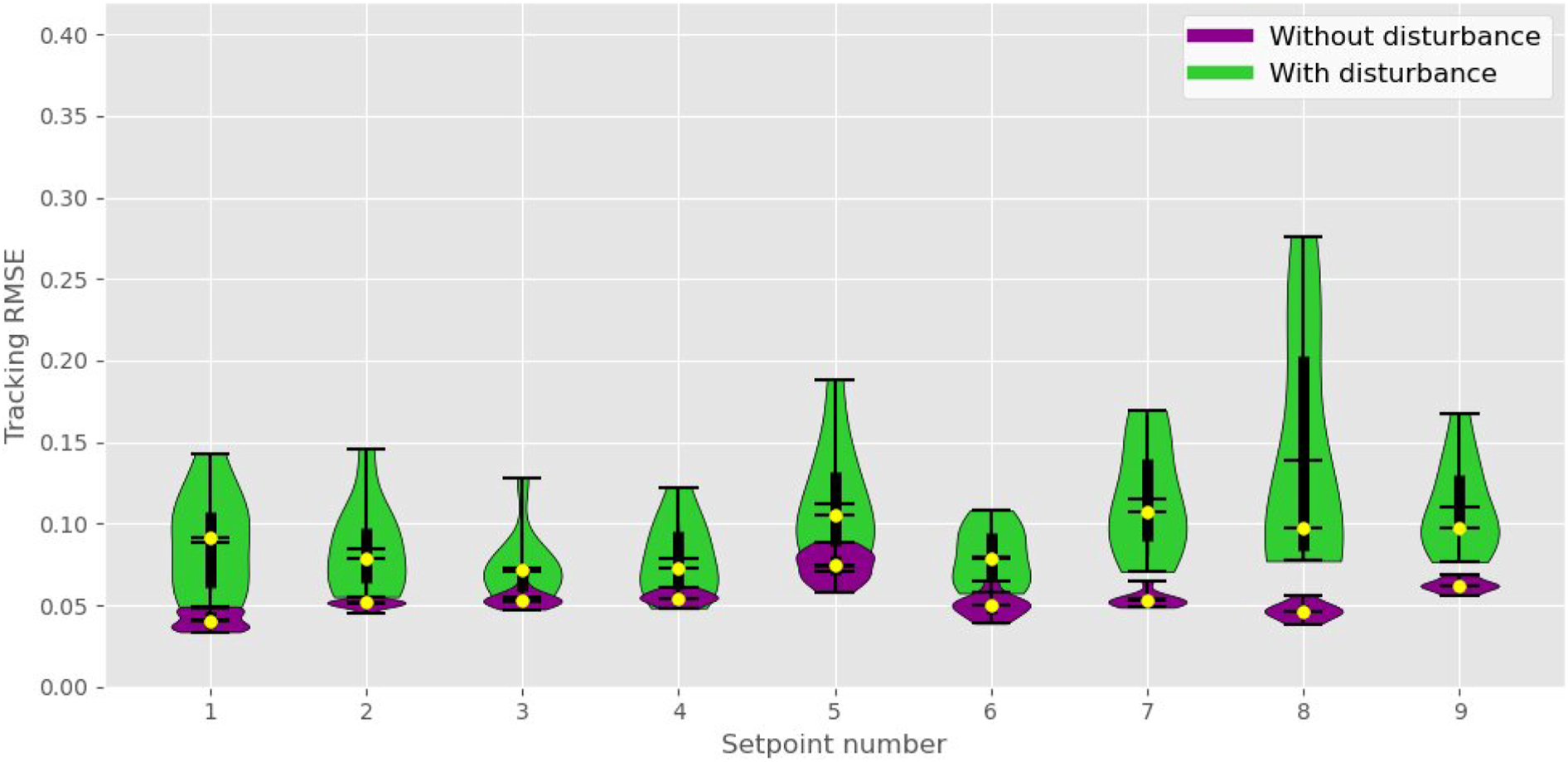
In terms of the Std of the RMSE (see Table 10 below), the LB controller outperformed the MB controller at every setpoint. On average, the Std of the RMSE against disturbance is 2.96 times smaller with our LB controller.

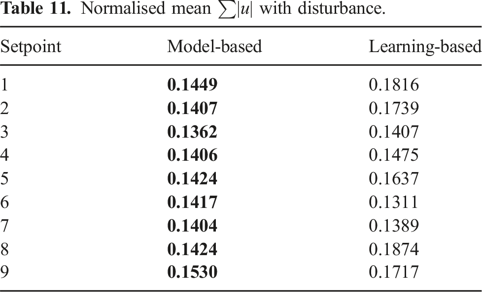
When considering the norm of the control inputs (see Table 11), we can now see that the LB controller required larger control inputs at all setpoints to stabilise the vehicle compared to the first environmental conditions. We believe that this result is explained by the successful detection of variations in the current disturbance. The attenuation of low-frequency disturbance is inversely proportional to the integral gain. Maximising the integral gain is a good heuristic to obtain a PID controller with good disturbance rejection. The LB controller can detect this change and increase the control parameters resulting in higher control inputs. Nevertheless, given the adaptive pole-placement design (Chaffre et al., 2021), the resulting gains of the PID controller are positively correlated. Thus, the derivative gain will also increase, which decreases stability margins. However, for pole values lower than 1, the proportional and integral gains vary exponentially while the derivative gain varies linearly (Chaffre et al., 2021). The LB controller successfully increases the proportional and integral gains while maintaining the same order derivative gain. This results in better disturbance rejection with similar smoothness in the control of the vehicle as suggested by the lower RMSE and std RMSE. On average, the LB controller consumed 9% more energy than the MB controller.

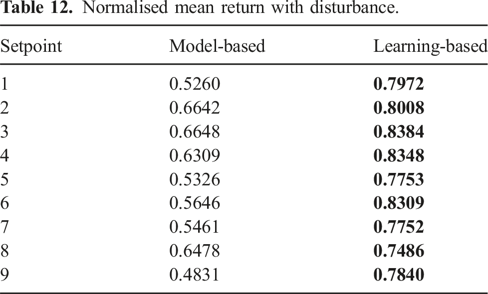
Finally, when taking into account the mean total reward generated per episode by the agents (see Table 12), we can that the LB controller also outperforms the MB controller at every setpoint. The normalised mean return of the LB controller was on average about 1.36 times higher than the MB controller. It is worth observing that the MB controller was not able to stabilise the vehicle while the LB controller was able to complete the task in this scenario.

This tendency is shown in the violin plots provided in Figure 11 where we can again see the median and quartile values computed over the 10 trials. The difference in performance is furthermore important against current disturbance.

Figure 11.

Illustration of the experimental performance of the controllers with current disturbance.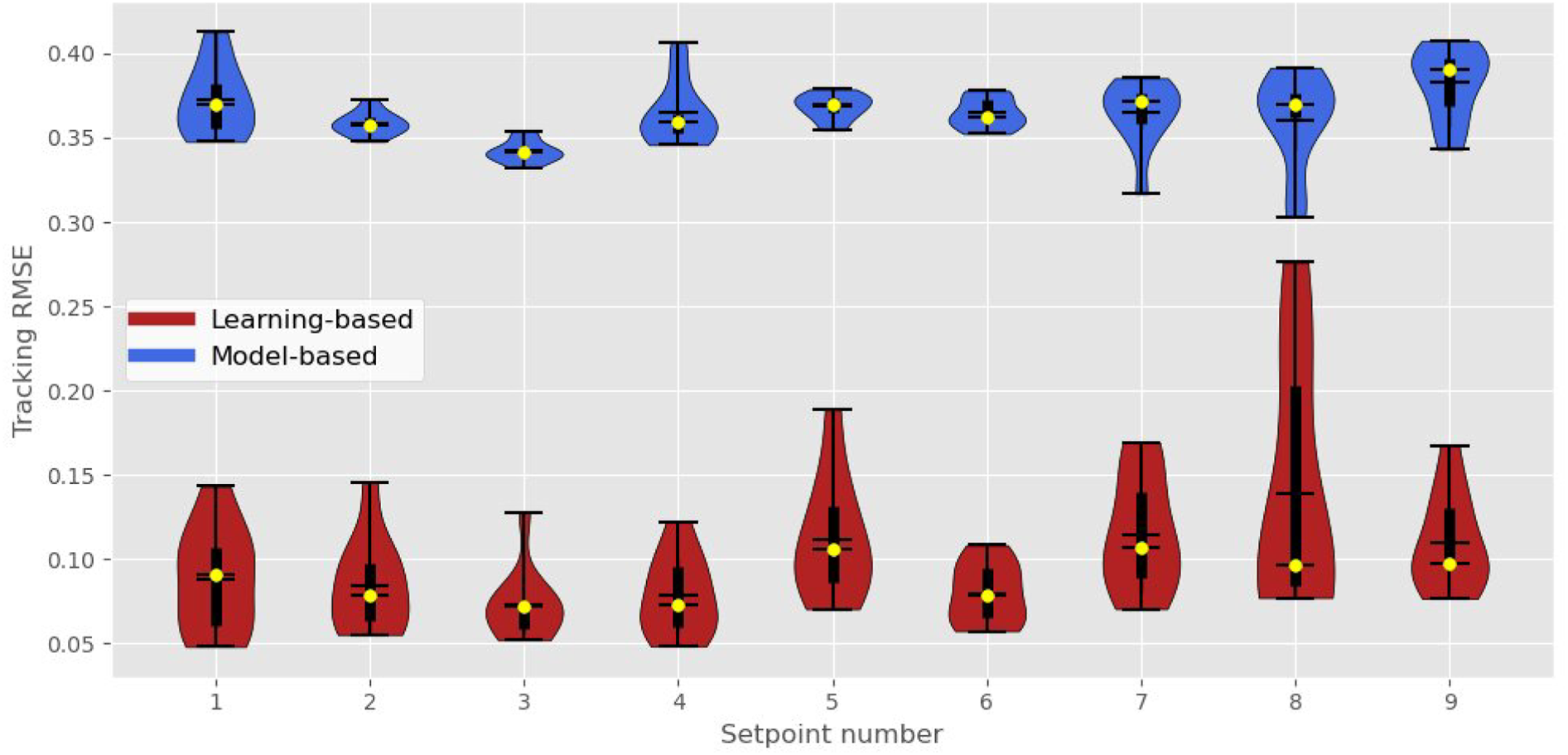

Figures 12 and 13 below provide the opportunity to compare the violin plots of the results for each controller. We can see that despite using a suboptimal simulated model of the AUV, the learning-based policy performed notably better when transferred to the real platform compared to its nonadaptive optimal counterpart.

Figure 12.

Example of the experimental performance of the MB controller without and with current disturbance.

Figure 13.

Example of the experimental performance of the LB controller without and with current disturbance.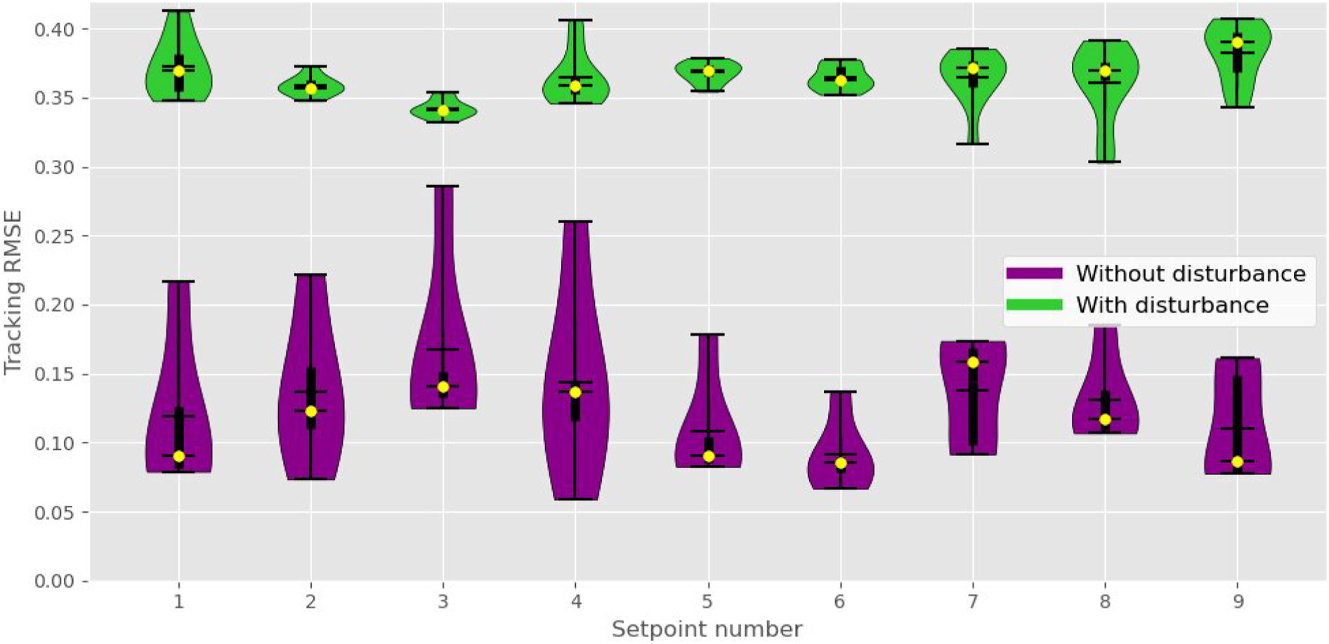

Figures 14–19 show the trajectories performed by both controllers for each DoF during an episode with current disturbance. These trajectories might not be representative of the mean performance of the controllers outlined in the previous tables, but they were chosen as they provide great insights into the controllers’ behaviour. Overall, we can observe that the proposed learning-based adaptive controller displayed a lower overshoot and is better at tracking the desired trajectory.

Figure 14.

Evolution of the position X. (a) MB controller and (b) LB controller.

Figure 15.

Evolution of the position Y. (a) MB controller and (b) LB controller.

Figure 16.

Evolution of the position Z. (a) MB controller and (b) LB controller.

Figure 17.

Evolution of the roll ψ. (a) MB controller and (b) LB controller.

Figure 18.

Evolution of the pitch θ. (a) MB controller and (b) LB controller.

Figure 19.

Evolution of the yaw ϕ. (a) MB controller and (b) LB controller.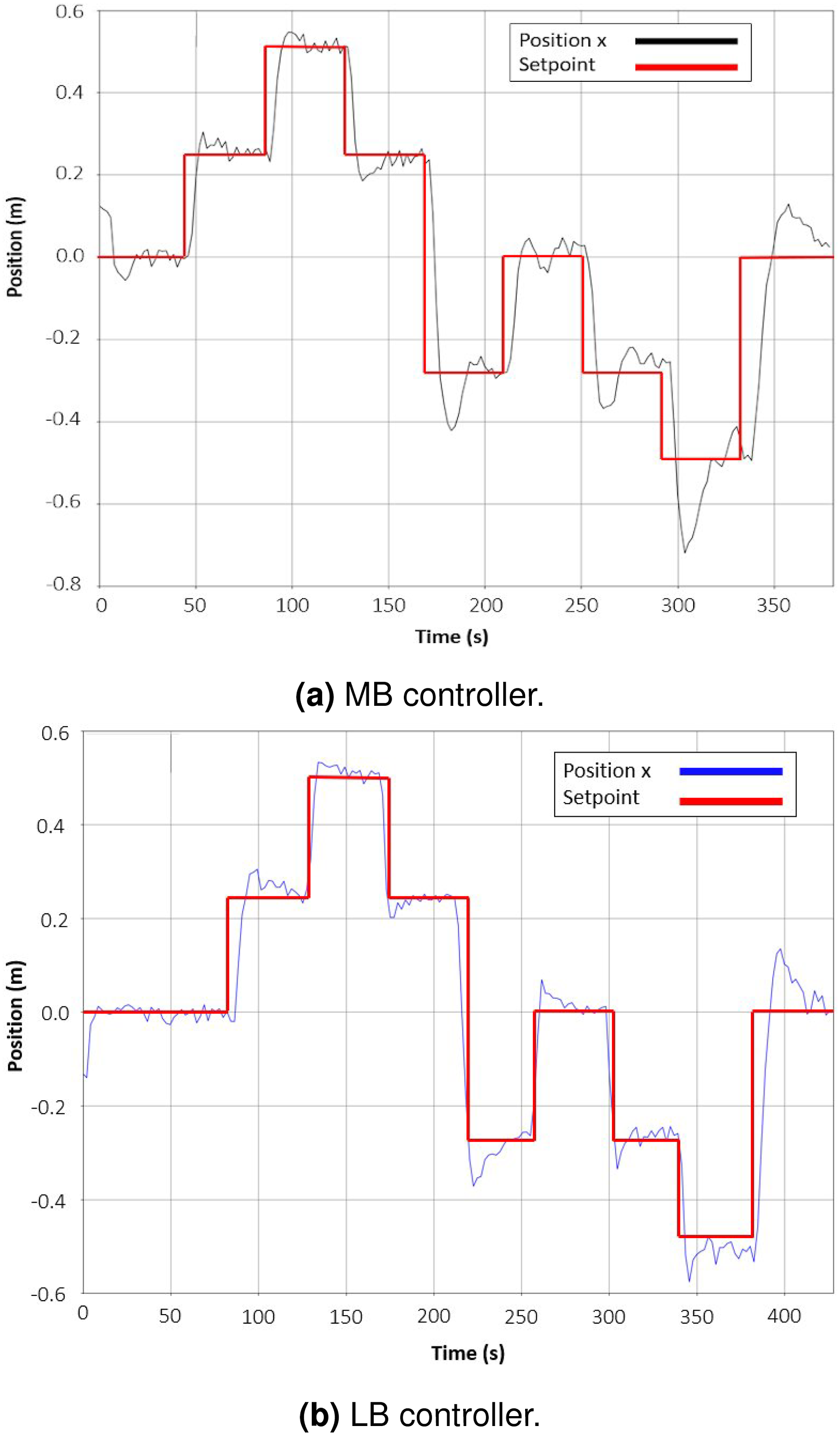

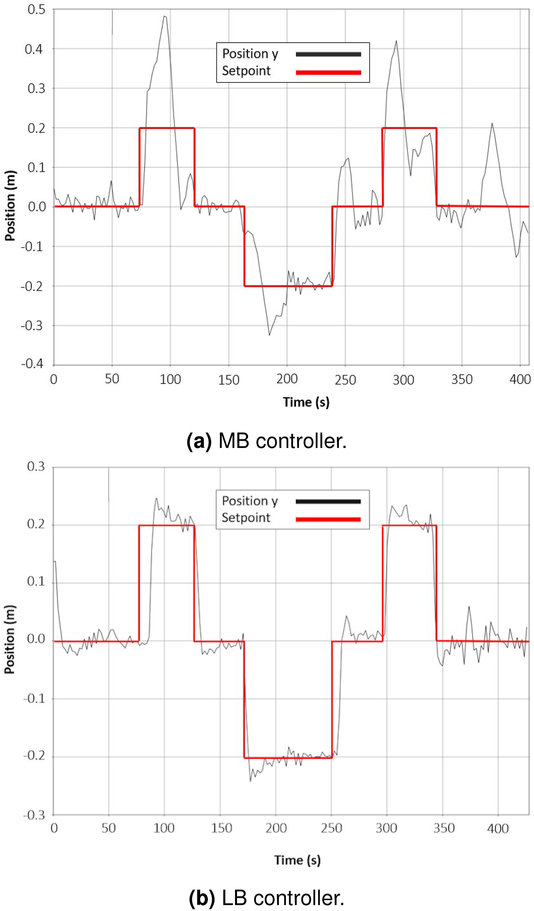
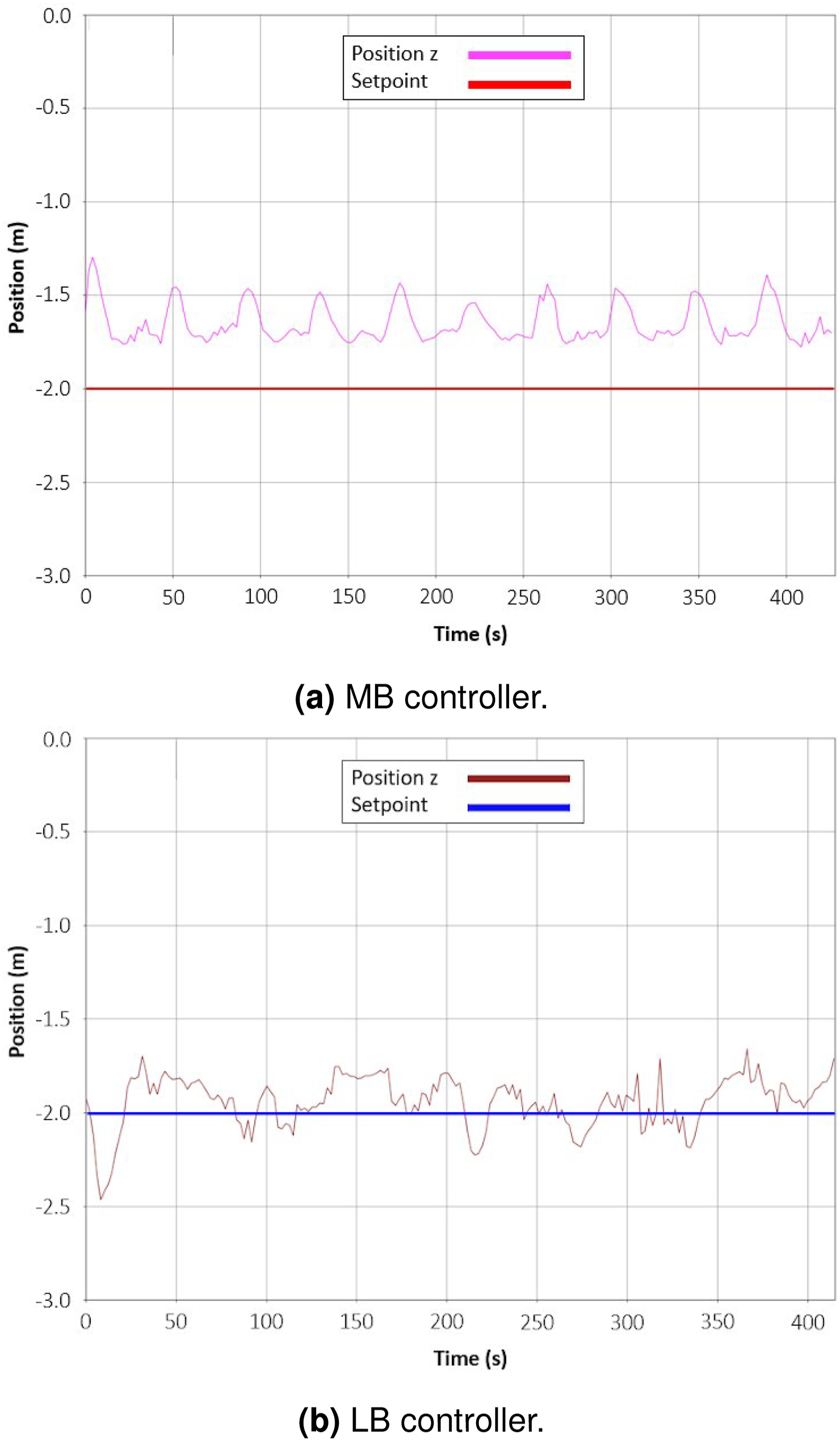
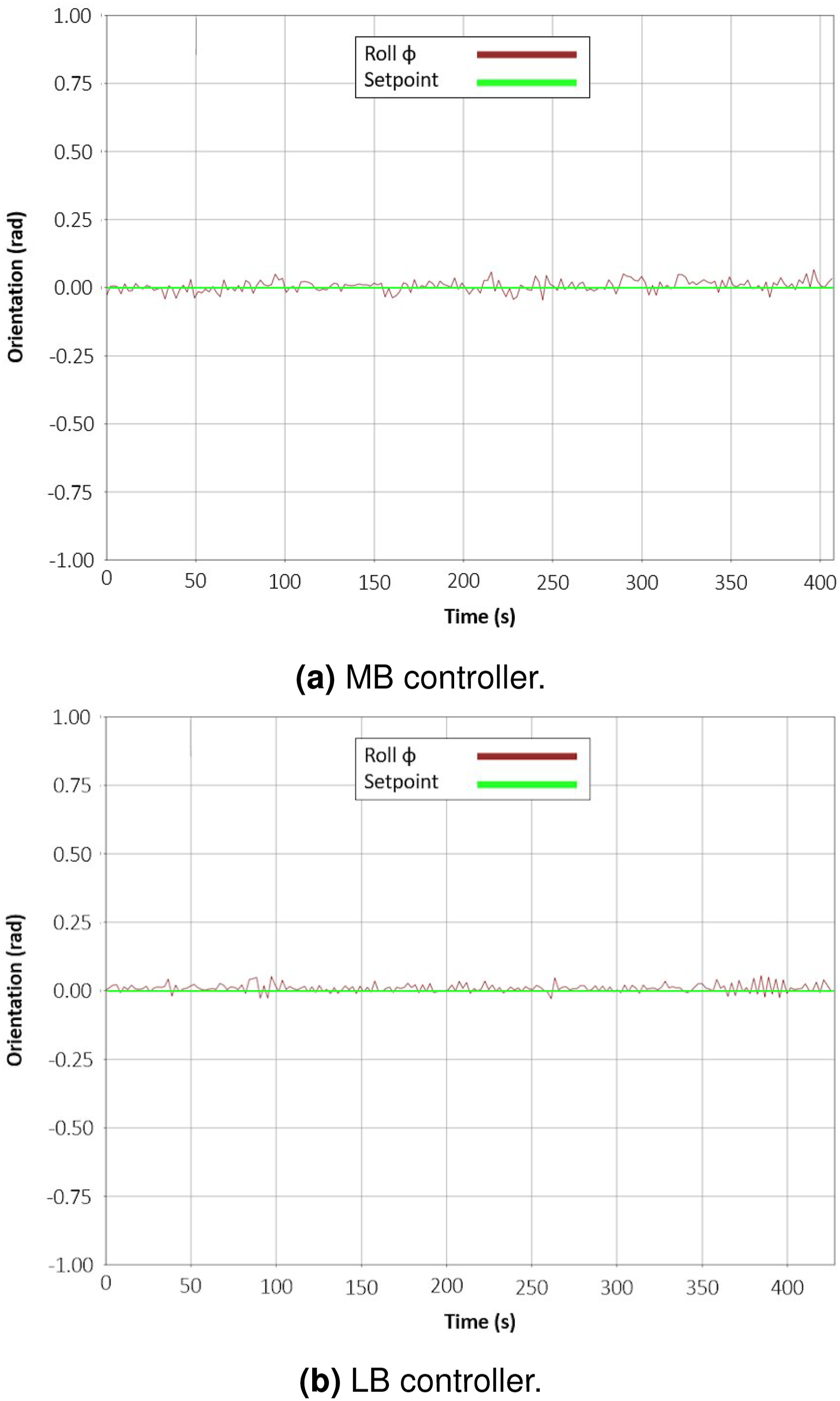
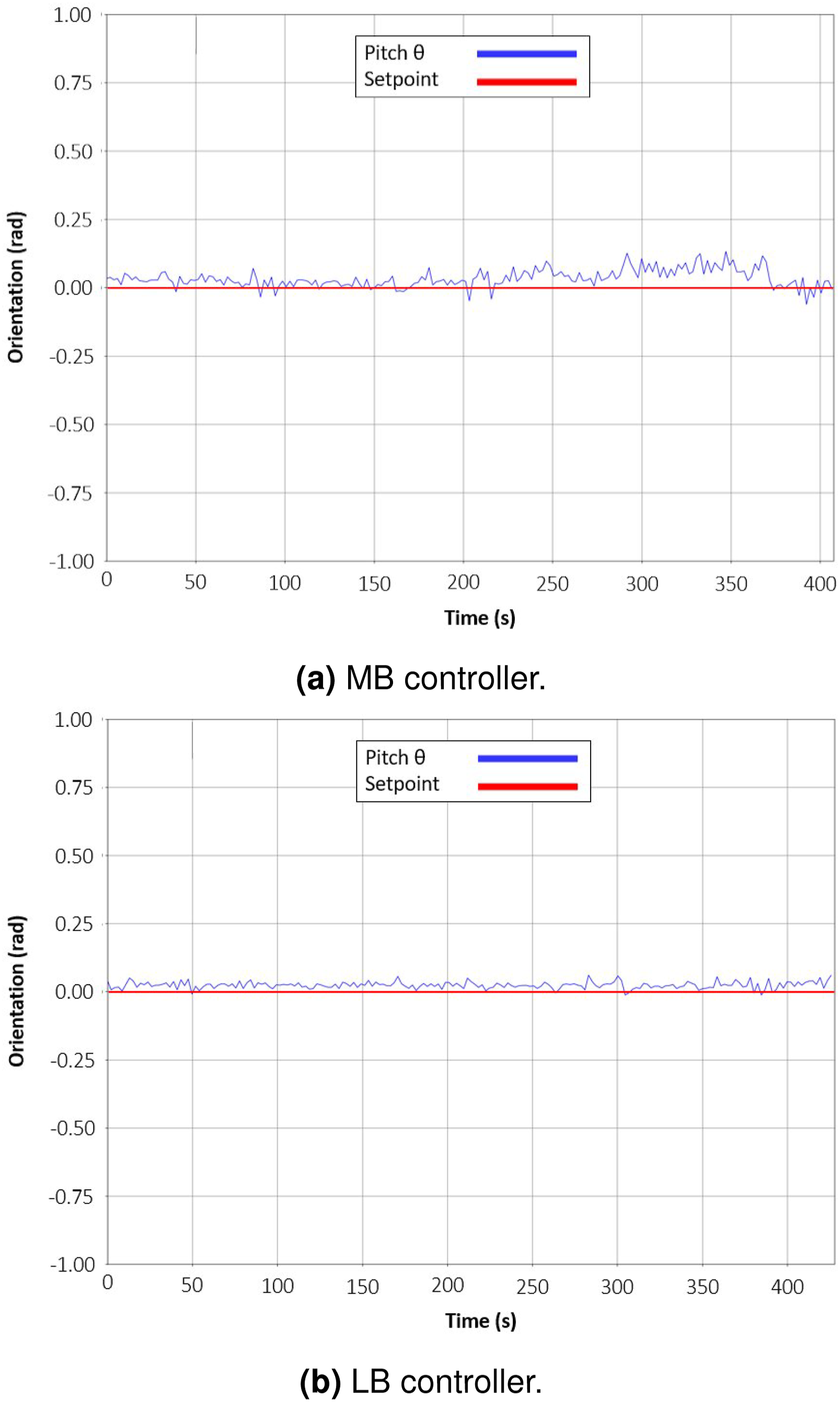
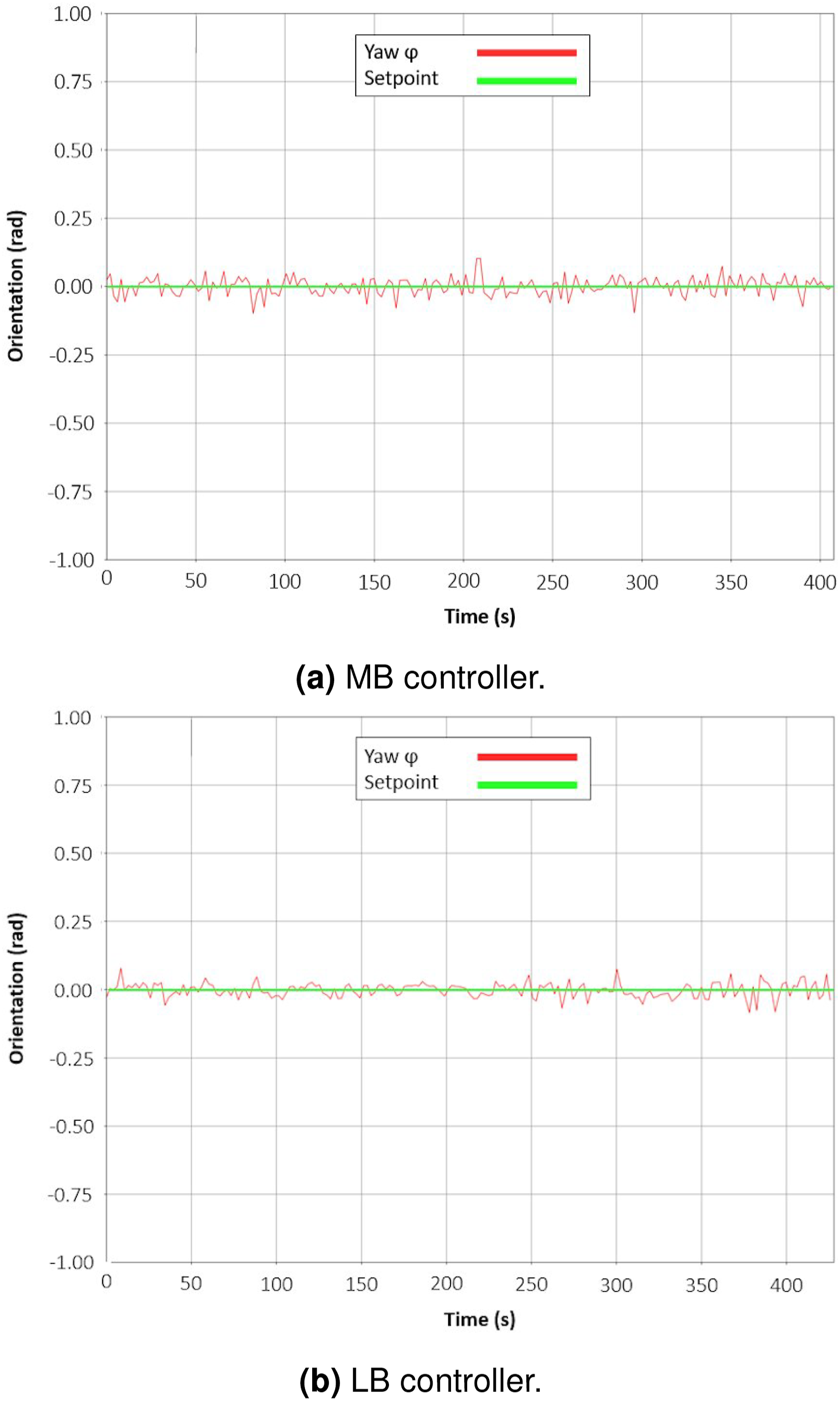
In Figures 14–16, we can see that the overshoot on the setpoint is smaller with the LB controller and, in this particular example, we can observe residual steady-state error for the depth z with the MB controller. In Figures 17–19, we can see that in terms of Euler angles, the LB controller is also better.

To conclude, we have presented here the results of an experimental evaluation. We evaluated the two controllers on a multi-station keeping task and in two distinct scenarios: without and with current disturbance. We have presented the resulting outcomes of this evaluation as the mean values of multiple key performance indicators obtained over 10 trials for each controller, emphasising about 280 min of real-life operating time. We have shown experimentally that the proposed LB adaptive controller consistently outperformed the MB optimal controller.

10. Discussion

Learning-based adaptive control provides an efficient way to cope with process variations by providing a model-free adjustment mechanism. However, so far their success at solving difficult AUV processes has been limited, mostly due to the partial observability of underwater environments. We have argued that the key to a successful sim-to-real transfer is to obtain good estimates of the Q-value function via Domain Randomisation (Chen et al., 2022) and Maximum Entropy DRL (Eysenbach and Levine, 2022).

We have provided a methodology to design a learning-based adaptive control system based on the PID control law, which represents the vast majority of in-use AUV control systems. We described how to combine this control structure with the Soft Actor-Critic and Automatic Temperature Adjustment mechanism that optimises a value and policy function, both represented by ANNs. Combining model-based control and model-free learning, we can compensate for the unobservable current disturbances.

Our main experimental validation was in the domain of manoeuvring tasks for AUV. Despite being trained on a different model of the vehicle under simulations, the resulting policy was still able to regulate the vehicle and displayed performance between 2 and 3 times higher (in terms of setpoint regulation) compared to the nonadaptive optimal model-based controller. This was possible thanks to the proposed learning-based architecture where DRL is used to learn to adapt to the overall dynamics of the process rather than learning the dynamics of a specific vehicle/process (i.e. end-to-end DRL).

This approach grants the control system the ability to learn how to adjust the control parameters against changes in the error signals, making it easier to transfer to a slightly different vehicle/process.

One question that deserves future investigation is the relationship between the process observability and the distribution shift problem in RL (Ghosh et al., 2021; Li et al., 2023). If this relationship were known, we could greatly reduce the overestimation problem (Kumar et al., 2019) of Deep Q-Learning. Some candidates for that are Distribution Constraints via Lyapunov Theory (Kang et al., 2022), improved Regularisation (Eysenbach et al., 2023a, 2023b), or Implicit Q-Learning (Kostrikov et al., 2022).

11. Conclusions

This paper investigated the application of learning-based adaptive control in the context of AUV disturbance rejection, yielding several noteworthy contributions, summarised as:

• A novel learning-based adaptive control architecture was introduced, designed for utilisation alongside traditional feedback control methods, such as PID controllers, resulting in a controller that is adaptable to changes at the same time that it maintains a backbone grounded on physical modelling of the plant.

• A comprehensive empirical evaluation was conducted by implementing and assessing the proposed learning-based adaptive controller alongside its nonadaptive, model-based counterpart on an actual AUV platform. Remarkably, despite sharing an identical controller structure, the learning-based approach exhibited substantial performance enhancements.

• This research contributed an analysis of the transferability of the policies learnt from simulation to the physical plant, wherein the learning-based adaptive controller, initially trained on a dissimilar vehicle model, demonstrated the capability to effectively stabilise the AUV in a real-world context, underscoring its adaptability and generalisability.

• An exploration into the correlation between the complexity levels of source and target domains led to the identification of a pivotal factor: domain randomisation. We observed that randomising environmental complexity, quantified by factors such as sea current disturbance amplitude and task difficulty, mitigated policy variance, thus elucidating a key mechanism contributing to the improved sim-to-real transfer.

Additionally, to facilitate the transition from simulation to practical deployment, we deployed the SAC algorithm with the Automatic Temperature Adjustment mechanism on a physical AUV, which (to the best of our knowledge) has not been done before in the context of AUV control. This improvement obviates the need for intensive and empirical reward scale parameter tuning, enhancing the method’s usability and efficiency for underwater vehicles.

Future work will focus on evaluating the proposed methods in an industrial-level application of an AUV operating in an open sea environment. Not only will this provide stronger evidence for the efficacy of the proposed work but also offer the opportunity to incorporate nonlinear model-based control structures to address underactuated situations in a more challenging setting.

To tackle the lack of accurate GPS in open sea environments, we plan to combine ultra-short baseline (USBL) methods with Doppler Velocity Log (DVL) sensors to build a robust estimate of the vehicle’s position and orientation through particle or Kalman filters.

From a machine learning perspective, future efforts will aim to optimise the policy directly on the vehicle during operation. Although Deep Policy Gradient (DPG) methods can be computationally demanding, hindering online training, a prospective step involves developing model-free policy optimisation methods using Evolution Strategies (Tavakkoli et al. (2024)). This approach would allow adjusting policy parameters online without the need for computing gradients.

A question for future investigation is whether the proposed algorithm could be trained and evaluated on diverse types of vehicles and tasks. Given that the focus is on regulating error variations rather than specific vehicle dynamics, the hypothesis is that a learning-based adaptive controller should be able to regulate unfamiliar vehicles as long as their underlying dynamics are not drastically different from the training vehicle. An example may be the fault-tolerant control we have started exploring in Lagattu et al., (2024)).

Furthermore, we anticipate that the design for station keeping could generalise to trajectory tracking, as the only fundamental difference lies in whether the setpoint is a function of time. Finally, to enhance stability, future work will explore control structures beyond PID, such as using a Linear Quadratic Regulator (LQR), Model Predictive Control (MPC), or L2-gain controllers, where Lyapunov stability is inherently incorporated in the optimisation resolution, providing more formal stability guarantees.