Sage Journals: Discover world-class research

Abstract

This paper deals with an experimental comparison between the proportional integral derivative (PID) control law and the adaptive nonlinear state feedback control, both applied on the AC-ROV underwater vehicle. The experimental results evaluate the closed-loop behaviour of the system under each controller in various operating conditions in order to compare how robust they are towards parameters' change and how they can reject external disturbances. It was concluded that the adaptive controller ensures a faster convergence and can adapt to a change of parameters as well as compensate for external disturbances. The PID needs to be retuned for every parameter change and is more sensitive to external disturbances.

Keywords

Underwater robotics Depth regulation PID controller Adaptive Controller

1. Introduction

Underwater vehicles have gained an increased interest in the last decades given the multiple operations they can perform in various fields. The recent development of such robots enlarged the range of tasks in environments considered as hazardous or dangerous. Lots of advantages in terms of operational cost and safety were brought with the usage of such vehicles in underwater inspection, as in various other tasks involving manipulation, assembly or repair of offshore structures [1, 2]. We are particularly interested in the category of tethered vehicles also called remotely operated vehicles (ROV). The teleoperation of these vehicles is difficult since the execution of the above mentioned tasks require the simultaneous monitoring of various parameters and degrees of freedom. Automated depth control facilitates the missions involving systematic longitudinal scanning such as the inspection of dams or ship hulls. Different challenges in controlling such systems arise from the inherent high nonlinearities and the time varying behaviour of the vehicle's dynamics subjected to hydrodynamic effects and disturbances. In fact, the model parameters are likely to change with the environment and the mission. For example, when the robot is required to manipulate objects or carry payloads, or when it is equipped with additional sensors, its weight, inertia, and drag change. Moreover, the buoyancy varies with the salinity of the water and the damping increases if some algae get a grip on the vehicle. Trajectory tracking involves also accounting for some expected or unexpected external disturbances such as waves that are common in shallow waters, or random obstacles that the vehicle might fail to avoid. It is therefore highly desirable to design and develop a controller able to deal with the inherent complex dynamics of the system while being able to properly compensate parameters changes and reject disturbances. Various approaches to solve this control problem can be found in the literature. Most of them aim at being robust and adaptive. In [3, 4] and [5], a robust ℋ_∞ control approach was proposed and tested on AsterX AUV (autonomous underwater vehicle) in simulations. The authors have tested this control scheme in situations where variations were brought to the mass of the robot and to the sampling time control interval. Other successful simulation results have been reported with the adaptive controller on the Phantom ROV [6] with 4 degrees of freedom in the aim of compensating persistent hydrodynamic terms in different frames of reference. The same approach was used in [7] where a more explicit description of the varying parameters and their plots was presented. Experimental results of this controller can be found in [8] where the AUV ODIN was tested in a pool with a constant current disturbance. Various chattering free sliding mode schemes have been applied on such systems to cope with heavy uncertainties and were experimentally validated in [9] where a fuzzy sliding mode controller was applied on the AUV-HM1 and in [10] where a higher order sliding mode was tested on an underwater vehicle prototype designed at the Cagliari University. Combining various techniques has also been studied with the usage of adaptive fuzzy sliding mode controllers for trajectory tracking and depth control as presented with numerical results in [11] and [12]. Intelligent control methods applying reinforcement learning or artificial intelligence can be found in [13, 14, 15] and [16] where simulation results are provided. An experimental study was reported in [17] where the robot ICTINEU AUV was subjected to reinforcement learning for a cable tracking application.

Comparisons among various controllers can be found in the literature through simulations. In [18] and [19] a comparison among adaptive controllers is reported. The former study shows robustness of each control law against measurements noises and parameters uncertainties while the latter one describes the ability of each adaptive controller to compensate for the currents and restoring forces. The sliding mode controller was compared in simulations to the Mu synthesis in [20] and to the robust adaptive fuzzy sliding mode controller in [11], in terms of trajectory following and measurement noise. In [21], four various model based controllers (adaptive and nonadaptive exact linearizing controllers, adaptive and nonadaptive nonlinear controllers) were experimentally compared to the PD controller in the case of a good and bad initial parameter estimation and in the case of thruster saturation. Trajectory following plots were shown only for the nonlinear controller. The study was based on the tracking error among the various controllers that shows a bad performance of nonadaptive controllers in presence of wrong model values and a degraded performance for all controllers in presence of a thruster saturation. This study lacks robustness tests to disturbances and parameter changes as well as illustrative plots. To the best of our knowledge, no detailed comparative experimental study between two controllers with various robustness tests has been performed. We propose in this paper to study the closed-loop system behaviour under a Proportional Integral Derivative (PID) controller and an adaptive nonlinear state feedback one. Our contribution lies in reporting an experimental evaluation of the effects of parameters changes and external disturbances on the closed-loop response of the system for the tethered underwater vehicle AC-ROV. For this purpose, the buoyancy and the damping parameters will be modified and external disturbances including a mechanical shock and waves, will be applied on the system. These scenarios will be conducted on each controller and results ranging from system response to control input, and changes in model parameters will be presented. This paper is organised as follows: in the second section we present the dynamic modelling of the system, the third section shows the theoretical aspects of both controllers to be compared, the fourth section presents the prototype and the experimental setup and in the fifth section the obtained experimental results and their analysis.

2. Dynamic modelling of the system

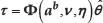
Throughout this paper, the variables in bold represent matrices and the ones in normal font represent scalars. By considering the inertial generalised forces, the hydrodynamic effects, the gravity, and buoyancy contributions as well as the effects of the actuators (thrusters), the dynamic model of an underwater vehicle in matrix form, using the SNAME notation and the representation proposed by Fossen in [22], is written as:

\begin{matrix} \dot{η} = J (η) ν \\ M \dot{ν} + C (ν) ν + D (ν) ν + g (η) = τ + w_{d} \end{matrix}

(1)

where v=[u,v,w,p,q,r]^T, η[x,y,z,φv,ψ] ^T are vectors of velocities (in the body-fixed frame) and position/Euler angles (in the earth-fixed frame) respectively. J(η) ∈ ℝ^6×6 is the transformation matrix mapping from the body-fixed frame to the earth-fixed one. The model matrices M, C , and D denote the inertia (including added mass), Coriolis-centripetal (including added mass), and damping respectively, while g is a vector of gravitational/buoyancy forces and moments, τ is the vector of control inputs and w_d the vector of external disturbances. In the case of our study, the vehicle will be moving at low velocities which makes the Coriolis terms negligible. Therefore, the dynamics (1) can be rewritten as:

M \dot{ν} + n (ν, η) = τ + ω_{d}

(2)

with n (v,η) = D(v)v + g (η)

Equation (2) describes the system in 6 degrees of freedom taking into account the 3 translations and the 3 orientations. The input vector τ ∈ ℝ⁶ considers 6 actions on the system to fully control it. In this paper, given the available sensors and instrumentation, we only study the dynamics of the vehicle in its translational motion along the z axis. Although the results concern only one DOF, this allows us to highlight each method's advantages and drawbacks throughout the experimental results. We can easily extract from Equation (2) our studied dynamics as:

M_{z} \dot{w} + D_{z} w - c o s (φ) c o s (ϑ) (W - B) = τ_{z} + w_{d_{z}}

(3)

The effects of gravitational and buoyancy forces are now brought to a single term which is a nonlinear combination between the weight W and the buoyancy B. τ _z is therefore the one dimension control input expressed in Newton and controlling the depth. It is given by:

τ_{z} = T K u

(4)

where u ∈ ℝ² is the vector of control inputs in volts (we have two thrusters acting on the degree of freedom of interest), K is the force coefficient in Newton per Volts and it has been previously identified trough experiments. T ∈ ℝ² is the actuators configuration matrix taking into account the position and orientation of the motors, thus allowing to determine the associated forces in the body-fixed frame.

3. Proposed control schemes

Our control objective is to achieve a depth regulation with a satisfactory closed-loop system response in spite of various external disturbances or parameters changes. For this purpose, we propose two different controllers: the Proportional Integral Derivative and an adaptive nonlinear state feedback. The former controller has been tuned using a method that minimises the ISTSE (Integral of Squared Time Multiplied by Squared Error) [23] while the latter one was tuned empirically so as to minimise the same criterion. For this purpose, the gains of this latter controller have been initially set to the same values than the optimised ones of the PID controller. Then, once the adaptation has been included, these gains have been finely adjusted to minimise the ISTSE criterion. Since each proposed scheme is expected to exhibit its best performance, the main characteristics and differences between these two controllers will be revealed throughout the proposed experimental scenarios even if a more thorough or slightly different tuning could be possible. In this study the single control input intended for the dynamics described in (3) will be computed. The indices (1) and (2) will be used for the gains of the PID and the adaptive controller respectively. General K_p, K_I, K_D will be used only to explain the mathematical description of each law.

3.1 Proportional Derivative Integral (PID) controller

3.1.1 Control law formulation

A classical PID controller has been used to achieve the desired depth regulation. The control input is given by:

τ_{z} = - K_{P_{1}} (z - z_{d e s}) - K_{I_{1}} \int_{0}^{t} (z - z_{d e s}) d t - K_{D_{1}} (\dot{z} - {\dot{z}}_{d e s})

(5)

where τ _z is the input in Newton to be applied along the z axis, K_p, K_I₁ and K_D₁ are positive constants gains representing respectively the proportional, the integral and the derivative gains, z is the measured depth, ż_des the desired one and z and z_des are their respective time derivatives.

3.1.2 PID Controller Design

The control input in Equation (5) is based on the well known mathematical description of the PID controller given by:

u (t) = K_{P} [e (t) + \frac{1}{T_{i}} \int_{0}^{t} e (t) d t + T_{d} \frac{d e (t)}{d t}]

(6)

with e(t) being the error signal, K_p the proportional gain, T_i the integral time and T_d the derivative time.

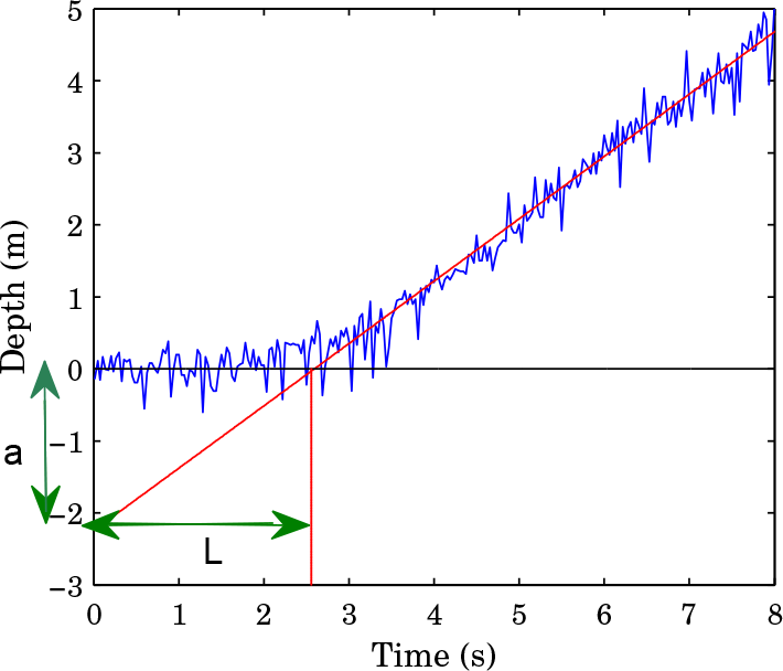
To tune the parameters of a PID controller, several methods exist in the literature such as Ziegler-Nichols, Cohen-Coon and Chien-Hrones-Reswick tuning methods. The depth behavior of an underwater vehicle can be approximated by an integral process with dead time. Many tuning rules for such systems can be found in [24] and [25]. Our system can therefore be approximated according to the following Integrator Plus Dead Time (IPDT) model:

G (s) = \frac{a}{s L} e^{- s L}

(7)

where the parameters L and a are the intersections of the tangent to the system step response with the x and y axes respectively (as illustrated in the Figure 1), and s is the Laplace variable.

Figure 1.

Graphical parameter estimation of an integrator model

In order to identify the parameters a and L of our vehicle's model, we have experimentally applied a thrust step along the z axis and we have observed the output behaviour. The experimental data normalized to a step input of 1N are displayed in Figure 2. By comparing the experimental step input response with Figure 1, we have found : L =2.6570 seconds and a=2.3 meters.

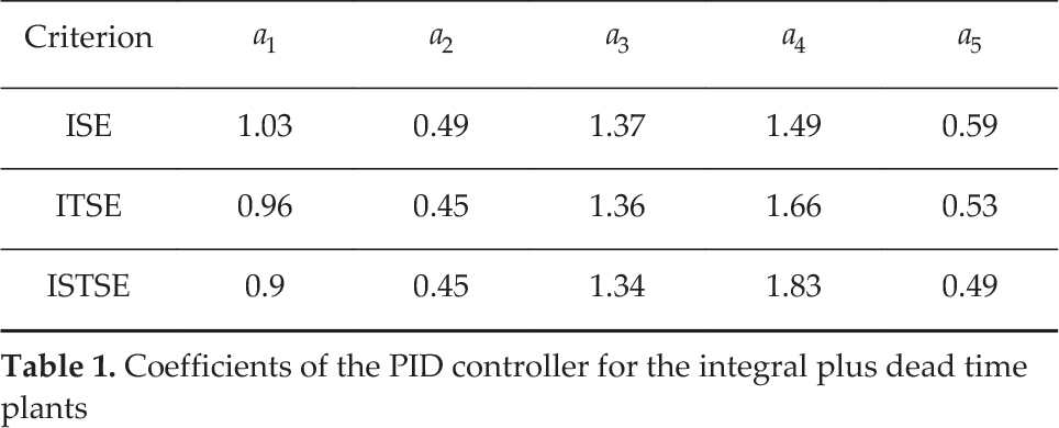
Once these two parameters have been found, according to [23], the gains of the PID controller can be computed from Table 1. This table holds all the coefficients for the design of either a PD or a PID according to different criteria (Integral of Squared Error (ISE), Integral of Time Squared Error (ITSE) and Integral of Squared Time multiplied by Squared Error (ISTSE)). The parameters a₁ and a₂ are used for the design of a PD whereas a₃ a₄ and a₅ are used for a PID. In this paper, we focus on inspection applications. We have chosen to optimise both speed and accuracy, and thus have decided to minimise the ISTSE criterion which is well suited for this purpose. Of course, this choice has to be made according to the targeted application and in other situations the optimisation of another criterion could be preferred.

Figure 2.

Scaled step input response of the AC-ROV to an input force of 1N

Using table 1, the computation of the gains of the PID controller becomes straightforward. With a₃=1.34, a₄=1.83, and a₅=0.49, and by letting $K = \frac{a}{L}$ , the gains are found to be:

K_{P_{1}} = \frac{a_{3}}{K L} = 0.58 K_{I_{1}} = \frac{K_{P_{1}}}{T_{i}} = 0.12 K_{D_{1}} = K_{P_{1}} T_{d} = 0.76

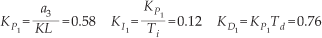
with T_i = a₄L and T_d=a₅L.

Table 1.

Coefficients of the PID controller for the integral plus dead time plants

Criterion	a ₁	a ₂	a ₃	a ₄	a ₅
ISE	1.03	0.49	1.37	1.49	0.59
ITSE	0.96	0.45	1.36	1.66	0.53
ISTSE	0.9	0.45	1.34	1.83	0.49

3.2 Adaptive nonlinear state feedback controller

3.2.1 Background

The adaptive state feedback controller is a state feedback controller with an adaptation part. It provides an online estimation of the unknown model parameters in order to ensure to the system a good trajectory following [22]. The control law is extracted from the dynamics of the robot presented in Equation (2) and rewritten as:

τ = \hat{M} a^{b} + \hat{n} (ν, η)

(8)

where the hat symbol denotes the parameter estimates, a ^b the body frame commanded acceleration, and n̂ (v, η) the estimate of n ( v, η ) in (2). Given that the dynamic model is linear in its parameters, the adaptive control law (8) can then be rewritten as:

τ = Φ (a^{b}, ν, η) \hat{θ}

(9)

where Φ is the regressor matrix and $\hat{θ}$ is the vector of the estimated parameters. The computed input is calculated in the body frame but the trajectory following is performed in the earth frame and therefore a^b is calculated from a simple transformation between the body and the earth frame given by:

a^{b} = J^{- 1} (a^{n} - \dot{J} ν)

(10)

where aⁿ is the commanded acceleration in the earth frame and J the transformation matrix. To guarantee that the error converges to zero, aⁿ is chosen as the following Proportional Integral Derivative (PID) control:

a^{n} = {\overset{..}{η}}_{des} - K_{P} \tilde{η} - K_{I} \int_{0}^{t} \tilde{η} dt - K_{D} \dot{\tilde{η}}

(11)

with $\tilde{η} = η - η_{des}$ and $\dot{\tilde{η}}$ is its first derivative, η_des is the desired trajectory and η_des is its corresponding acceleration.

The vector of the estimated parameters is updated according to the following update law:

\dot{\hat{θ}} = - Γ Φ^{T} (a^{b}, ν, η) J^{- 1} y

(12)

where Γ is a diagonal positive definite matrix representing the adaptation gain, J the transformation matrix, and y the combined error defined as:

y = c_{0} \tilde{η} + c_{1} \dot{\tilde{η}}

(13)

c₀ and c₁ are constant positive gains chosen according to the algorithm presented in [22] which states that the error on the trajectory, represented by y , is guaranteed to converge to zero by applying Barbalat's lemma. It has to be mentioned that the convergence of y is only possible when the parameters also converge. Moreover, if the parameters are not adequately initialised (for instance if their initial values are too far from the true values), they might never converge, thus leading to instability of the plant. It is also important to note that a good parameter convergence is more guaranteed to occur when the followed trajectory is rich enough to excite the parameters under study [26], However, parameters will converge to a set of values that allow trajectory following. Moreover, under the assumption of a good initialisation, the parameter vector is seen to be convergent according to Barbalat's lemma as shown in the proof of stability found in [22].

3.2.2 Case of the depth control

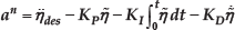
Given the available sensors and actuators with which our underwater vehicle is equipped, we have chosen to study a trajectory varying along the heave direction. The vector of parameters to be estimated includes M_z which is the third diagonal element in the inertia matrix, D_z the third diagonal element in the damping matrix, and (W – B) the parameter representing the difference between the weight and the buoyancy. Even if the addressed problem concerns depth control, it is worth to note that this study can be easily generalised to more degrees of freedom. From equations (8) to (13), we extract the explicit formulation of our controller as:

τ_{z} = Φ \hat{θ}

(14)

with the vector of the estimated parameters being:

\hat{θ} = [\begin{matrix} {\hat{M}}_{z} \\ {\hat{D}}_{z} \\ \hat{W - B} \end{matrix}]

(15)

the regressor matrix:

Φ = [Φ_{m} Φ_{d} Φ_{g}] = [a_{z}^{b} w - c o s (ϑ) c o s (φ)]

(16)

the commanded acceleration in the earth frame:

a_{z}^{n} = - K_{P_{2}} (z - z_{d e s}) - K_{I_{2}} \int_{0}^{t} (z - z_{d e s}) d t - K_{D_{2}} \dot{z}

(17)

the commanded acceleration in the body frame:

a_{z}^{b} = c o s (φ) c o s (ϑ) (a_{z}^{n} - (- q . s i n (ϑ) - p . c o s (ϑ) s i n (φ)) w)

(18)

the parameter adaptation law:

\dot{\hat{θ}} = - Γ Φ^{T} . c o s (φ) c o s (ϑ) . y_{z}

(19)

and finally the combined error:

y_{z} = c_{0} (z - z_{d e s}) + c_{1} (\dot{z})

(20)

Since we are performing a regulation around a desired depth, ż_des and z̈_des are equal to 0.

Finally, given the configuration matrix T and the force coefficient K explained in Equation (4), the control input can be expressed as:

u = \frac{T^{- 1} τ_{z}}{K}

(21)

3.3 State variables measurement and estimation

From our dynamical model (3), it appears that the used state variables are w, z, and ż. z is obtained from the depth sensor, whose data will also serve for the estimation of ż. For that, the proposed solution is based on an Alpha-Beta observer [27] described hereafter. From the estimation of ż, w will be found using the transformation between the earth frame and the robot frame. The Alpha-Beta observer is a simple observer formulated for state estimation in a closely related fashion to the well known Kalman Filter. Its main advantage is its independence from the system model which makes it easily implementable. The aim is to estimate the two internal states of a system where one state is the derivative of the second (case of many robotic systems). We consider the two states as being a position and a velocity, and then we use a two-step-algorithm: the first step is the estimation of the states using basic dynamics and the second step is the update of this estimate using the error computed from the position measurements and two constants α and β tuned empirically. The estimation step is formulated by the following:

\begin{matrix} c {\hat{x}}_{k} = {\hat{x}}_{k - 1} + Δ T . \\ {\hat{v}}_{k - 1} {\hat{v}}_{k} = {\hat{v}}_{k - 1} \end{matrix}

(22)

where k is the iteration, ΔT the sampling time, and x̂_k and v̂_k the two estimated states at instant k.

The update step is written as:

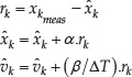
\begin{array}{l} r_{k} = x_{k_{m e a s}} - {\hat{x}}_{k} \\ {\hat{x}}_{k} = {\hat{x}}_{k} + α . r_{k} \\ {\hat{v}}_{k} = {\hat{v}}_{k} + (β / Δ T) . r_{k} \end{array}

(23)

where r_k is the residual error, $x_{k_{m e a s}}$ is the measured position and α and β are two constants between 0 and 1. In our case the position is the depth z updated with the pressure sensor and the estimated velocity is ż.

4. Real-time experimental setup

4.1 Modified AC-ROV experimental platform

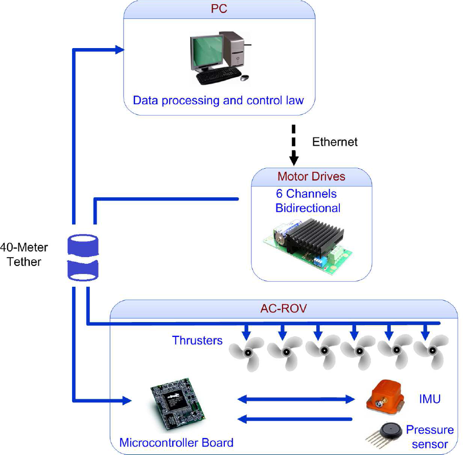
The AC-ROV (cf. Figure 3-(a)) is an underactuated underwater vehicle, whose propulsion system consists of six thrusters (DC motors + propellers) controlling five degrees of freedom. These actuators allow controlling the vehicle's orientation in pitch and yaw as well as all translational motions along the three axes (x, y and z). The yaw control is provided thanks to the differential speed control of the thrusters 1,2,3, and 4 (cf. Figure 3-(a)). These four thrusters also control the translation along x and y axes. Pitch control is obtained using thrusters 5 and 6, whereas the roll is left uncontrolled. However, the roll dynamics remains stable due to the positive damping parameter D_xx and because the centre of gravity is situated below the centre of buoyancy. The translational motion along the z axis is regulated by decreasing or increasing the combined speed of thrusters 5 and 6. The axes of the vehicle are shown in Figure 3-(b). For measurement purposes, our prototype is equipped with various sensors. A 6 DOF (Degrees of Freedom) MEMS based IMU (Inertial Measurement Unit) is fixed inside the body of the AC-ROV in order to be able to measure roll, pitch, and yaw. A pressure sensor allows depth measurement. To pre-process and transmit the sensors' data to the PC, a microcontroller board is used (cf. Figure 4). Once the control law has been computed by the control PC, the values of the control inputs are transmitted to the power stage through a dedicated microcontroller board. Then, 6 PWM modulated signals are sent to the actuators of the AC-ROV through the tether. The control software has been developed using C++ language under Windows Operating System. Figure 4 shows a schematic view summarising the various components of the vehicle's hardware and their interactions.

Figure 3.

Description of the Prototype, a: AC-ROV underwater vehicle and orientations of the forces produced by the 6 thrusters, b: AC-ROV Reference Frames (X_iY_iZ_i: earth fixed frame, X_bY_bZ_b: body fixed frame)

4.2 Conditions of the experiments

The experiments have been performed in a 4m³ water tank. The tether has been sufficiently unrolled in order to avoid additional drag to the dynamics of the vehicle. The feedback gains computed for each of the control laws and used in nominal conditions, have been kept unchanged during all the experiments despite some eventual changes in the physical system (AC-ROV) or its environment in order to evaluate the robustness of each controller. The noisy data of the depth measured by the pressure sensor are filtered using a second order Butterworth filter. The information concerning the velocity in the z direction is estimated by an Alpha-Beta observer with α =0.15 and β =0.045, as described in section 3. Figure 5 displays the experimental test-bed.

Figure 4.

Schematic View of the Hardware Architecture of AC-ROV Prototype

Our parameter vector has been initialised with our rough initial knowledge of the system. The gains used in the experiment are shown in the table below.

Table 2.

Parameters values of adaptive controller used in the experiments

Parameter	Value	Parameter	Value
$K_{P_{2}}$	0.5	c ₁	0.15
$K_{I_{2}}$	0.45	$M_{z_{i n i t i a l}}$	3 kg
$K_{D_{2}}$	0.1	$D_{z_{i n i t i a l}}$	14 N.s/m
Γ	1.5	(W – B) _initial	1 N
c _o	0.15

5. Experimental results

In this section the obtained experimental results will be presented and discussed. The controllers detailed in section 3 have been used to control the underwater vehicle described in section 4. We will start by explaining the different scenarios performed to test the two proposed controllers and then we will analyse the obtained results presented through Figures 7 to 17. The vehicle is regulated to reach a depth of 0.35 m when starting from a static surface position. On the depth response figures, the light grey lines represent the noisy measurements of the sensor, the thick black lines the filtered data and the dashed ones the desired regulated depth position. The evolution of the control inputs, generated by the actuators 5 and 6 controlling the movements along the z axis are also plotted for each scenario. Finally, Figure 17 shows the evolution of the parameter (W – B).

5.1 Proposed experimental scenarios

Three experimental scenarios were performed, namely:

i. Scenario 1: Control in Nominal Conditions:

The objective of this scenario is to control the depth of the AC-ROV without any external disturbance. The gains for each controller have been tuned to accommodate this case and were kept unchanged for the rest of the experiments.

ii. Scenario 2: Robustness towards External Disturbances

The following external disturbances are considered:

a. Punctual External Disturbance:

In this scenario, when the robot reaches its steady state position, a vertical mechanical impact is applied to the vehicle, pushing it downwards. The objective of this experiment is to evaluate the ability of the controllers to drive the system back to its regulated position. As it was experimentally impossible to reach a perfect repeatability of the impacts, we repeated each test at least ten times consecutively for each controller. To allow a fair comparison of the controllers, the indicated recovery times, as well as overshoot values, and residual oscillations correspond to the means of the measured values during the series of impacts. The figures corresponding to this scenario have been selected within the set of figures so as to best fit the mean behaviour.

b. Persistent External Disturbance (Waves):

With the launching of the test, waves were generated manually by periodically disturbing the environment of the pool which created waves of approximately 15 cm amplitude. The two proposed controllers will be tested and compared in this situation where the controlled system is subject to this persistent external disturbance and deduce which one could be more suitable for applications performed in shallow waters, where waves are likely to be present.

iii. Scenario 3: Robustness towards Modelling Uncertainties

In this scenario two uncertainties on two parameters will be considered, namely:

a. Change in Buoyancy:

The physical system has been changed by the addition of a rectangular piece of polyester as shown in Figure 6-(b) introducing a change of buoyancy of approximately +0.32 N and bringing a variation of 32% to the parameter (W – B). The aim of this modification is to impede the motion of the system downwards due to its new tendency to float. The objective of this scenario is to see whether the proposed controllers are sufficiently robust to compensate this uncertainty and keep the performance of the controlled closed-loop system.

b. Change in Damping:

As before, the physical system has also been changed by the addition of a floating rectangular ruler on the top of the vehicle as shown in Figure 6-(c) to increase the damping.

As before, we would like to study the effects of this change on the response of the system and evaluate the performance of the proposed two controllers.

Figure 5.

View of the AC-ROV Experimental Test-Bed: ①: Control PC, ②: External hardware case, ③: Power Input, ④: Switch, ⑤: Emergency stop button, ⑥: Video in, ⑦: AC-ROV tether in, ⑧: Ethernet cable, ⑨: Video Capture, ⑩: 40-metre tether, ⑰: AC-ROV

Figure 6.

View of the AC-ROV in different configurations: a: Nominal conditions, b: Buoyancy change, c: Damping change

5.2 Control in nominal conditions

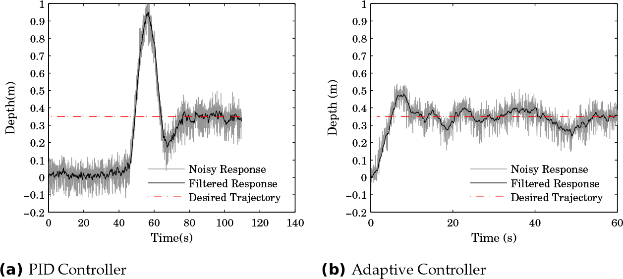
Figure 7 displays the evolution of the controlled vehicle's position for each of the proposed controllers. The PID controller in Figure 7-(a) needs around 80 seconds to reach steady state with an overshoot of 57%. Note that the delay of 40 seconds, noticed in Figure 7-(a), is caused by the time needed for the integral part to compensate the floatability of the robot (W – B) ≈ – 1 N). The adaptive controller reveals to be much faster and converges to the desired depth in 20 seconds with an overshoot of 28%. The settling time of this controller also coincides with the time needed for the parameter (W – B) to converge to its steady state value (cf. Figure 17-(a)). The evolution of this parameter is depicted in Figure 17-(a) and reaches a steady state value of −0.97 N.

The other two parameters did not evolve noticeably and hence were not represented. The reason of this latter observation lies behind the idea of enough parameter excitation that needs to be present in order to induce changes. The suggested trajectory excites mainly the parameter (W – B) which has a big effect on the dynamics of the vehicle. The initial parameter of M_z was carefully initialised since it was only required to weigh the robot. Indeed, the added elements shown in Figures 6-(b) and 6-(c) to increase the buoyancy and the damping respectively have a negligible weight. As for the parameter D_z, its rough initial estimate was enough since the vehicle moves at low velocities. As explained in section 3, assuming that the parameters are adequately initialised, they will converge. Once they have converged for the first time, it is convenient to record the values of this “nominal” set of parameters and to initialise them with these values for the next experiments. If we had not initialise them to these values, this would have simply induce a delay (convergence time of the parameters) but the comparison with the PID would not have been fair. The convergence of parameters that have been initialised with erroneous values will be illustrated by the results of scenario 3.

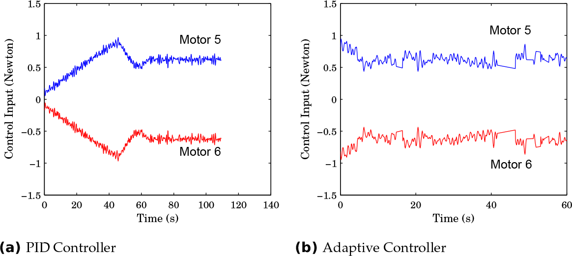
The maximal admissible force that can be generated by the motors is F = 2 N and we can notice from the curves of Figure 8 that this limit has not been exceeded and that the control force oscillates around a steady state value of 0.5 N for both controllers. We notice though that the control input exhibits larger oscillations (noise) in the case of the adaptive control. This point is important as it not only increases the power consumption (this is however not critical for tethered vehicles like ROV), but it also increases the thrusters' fatigue. This noise in the control inputs is mainly due to the noisy depth measurement (even when filtered) and to the derivative term of the controller. The possible solutions of this problem are indicated in the conclusion of the paper.

Figure 7.

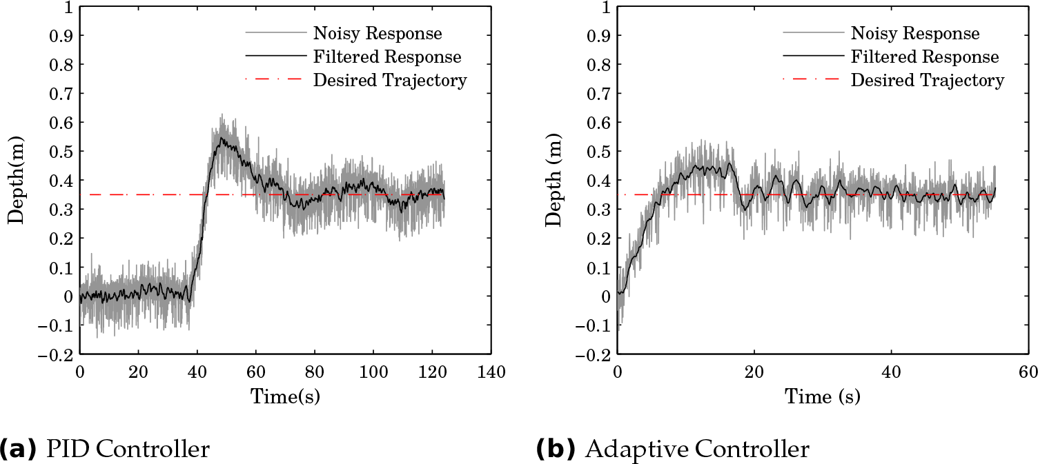
Depth Response in Nominal Regime

Figure 8.

Control Input in Nominal Regime

5.3 Robustness to external disturbances

5.3.1 Punctual external disturbance

As specified earlier, series of mechanical impacts have been applied on the vehicle after it has reached steady state (cf. Figure 9). For the PID controller, the mean recovery time was of 30 seconds against 25 seconds for the adaptive controller. The system responses of both controllers are similar even though we can notice larger oscillations around the regulated depth with the PID after the recovery from the disturbance was achieved. The control inputs shown in Figure 10 reveal an important overshoot with the adaptive controller, while the PID witnesses a decrease in its commanded input in absolute value. The former controller had a sudden change in its parameters leading to an overshoot of 1.5 N in its control input, while the latter was compensating for the induced error by sending a lower order to the thrusters. In this case, the PID controller seems to behave better in terms of energy consumption.

Figure 9.

Depth Response in Presence of a Punctual Disturbance

Figure 10.

Control Input in Presence of a Punctual Disturbance

5.3.2 Persistent external disturbance (Waves)

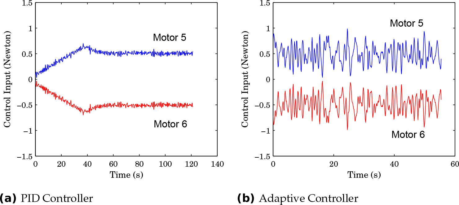
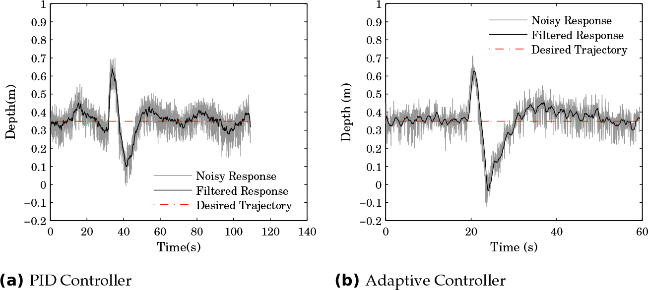
The obtained results of this scenario are depicted in Figures 15 and 16. Figure 15 shows the system response of the robot in presence of disturbing waves. Varying oscillations around the regulated depth are observed with both controllers. However, those of the PID controller are more significant with an average of 20 cm amplitude. It is worth to notice that the adaptive controller exhibits smaller oscillations with 10 cm of average amplitude which means that it was able to partially attenuate the effect of the waves in order to remain around the value of the desired depth. The oscillations observed in Figure 15-(a) are reflected in Figure 16-(a) where the control input is observed to be oscillating without converging to a steady state value. In Figure 16-(b), less severe oscillations can be observed on the control signals generated by the adaptive controller.

5.4 Robustness to modelling uncertainties

5.4.1 Change in buoyancy

The additional buoyancy incorporated in the system disturbs in a persistent way the motion of the vehicle that would tend to float more. The PID controller in this case responded with a delay of 35 seconds and an overshoot of 128%; furthermore oscillations of approximately 10 cm can clearly be observed around the desired depth (cf. Figure 11-(a)). Its control input seems to be similar to the nominal case except that it stabilises to a steady state value in a steeper manner with some small oscillations. We notice in this scenario a new delay in Figure 11-(b) when applying the adaptive controller. The delay is of 8 seconds and the settling time is of 40 seconds compared to 20 seconds in nominal conditions. This can be explained with the necessary time to adapt the parameter to the change and converge to its new steady state value of −1.18 N which also took 40 seconds to be reached (cf. Figure 17-(b)). The added buoyancy is found to be 0.21 N (−0.97–(−1.18)=0.21 N) when comparing the steady state values of the parameter (W – B) in Figures 17-(a) and 17-(b). This value of 0.21 N is close to the real one (0.32 N) by 65%. It is worth to note that adaptive controllers do not necessarily ensure the convergence of the updated parameters to their desired values [26] in order to obtain the convergence of the system to its desired position. The control law detailed in section 3.2 ensures the boundedness of the parameters but not necessarily their convergence to the real values. Concerning the control inputs generated by this controller, and depicted in Figure 12-(b), we can observe that the robot's actuators are exerting more effort and they oscillate around a mean value of 0.65 N. These oscillations are seen to be larger than with the PID case. This profile reveals the additional difficulty experienced by the motors in order to immerse the vehicle.

5.4.2 Change in damping

Similarly to the previous scenario, a change in the physical system was considered. It was integrated to damp the dive of the vehicle as illustrated in Figure 6-(c). The PID controller in Figure 13-(a) starts reacting at around 40 seconds and displays an overshoot of 171% but reaches steady state after 80 seconds. The required control input generated by this controller (cf. Figure 14-(a)) has a maximal value of 0.9 N and converges to a steady state value of 0.55 N after a small oscillation matched with the oscillation observed in the response of the system. The adaptive controller stabilises the system with a settling time of 20 seconds and a small overshoot of 28% like the nominal case but the oscillations around the desired depth are more important. The response could have been improved with a better excitation of the parameter D_z.

Figure 11.

Depth Response in Presence of a Buoyancy Change

Figure 12.

Control Input in Presence of a Buoyancy Change

Figure 13.

Depth Response in Presence of a Damping Change

Figure 14.

Control Input in Presence of a Damping Change

Figure 15.

Depth Response in Presence of Waves

Figure 16.

Control Input in Presence of Waves

Figure 17.

Evolution of the Parameter (W-B)

5.5 Summary of comparison between the proposed controllers

Table 3 below summarises the comparisons performed above between the two proposed controllers for different scenarios. Some relevant criteria have been chosen to perform this comparison which has been done in a qualitative and quantitative way depending on the criterion. It can be easily seen that the adaptive controller drives the system to steady state faster than the PID controller. Indeed, its closed-loop response has a settling time of approximately three times smaller than the case of the PID controller. This difference can be explained (as mentioned before) by the fact that the PID controller needs some time for its integral action to counterbalance the effect of the floatability. The adaptive controller needs a certain time to converge its parameters to their steady state values. However, this time depends on the adaptation gain and can therefore be shortened by increasing this design parameter. However, it is known that the adaptive control is not robust when the adaptation gain is set to be high and that justifies the reasonable choice of Γ =1.5 (see Table 2). The settling time of the closed-loop system controlled by the PID is around 60 seconds in the nominal case, however it increases to 80 seconds when considering the uncertainty on damping. In the case of the adaptive controller, the settling time is around 20 seconds but it doubles when an uncertainty on buoyancy is considered. Indeed, this unexpected uncertainty will lengthen the necessary time for the parameters to converge to their steady state values. Therefore the control input will be changed accordingly which affects the settling time of the closed-loop system. The PID controller always exhibits large overshoots when any kind of change is introduced to the system, while the adaptive controller stays around the performance of its nominal conditions thanks to the adaptation of its parameters. Regarding the precision of the output response, it is worth to note that the depth sensor used has an uncertainty of 5 cm and that's why the steady state oscillations were meant to be quantitatively indicated. The adaptive controller requires more energy than the PID controller and this can be shown from the more relevant force generated by the thrusters. This behaviour can be explained by the fact that the adaptive controller remains faster and more robust to all kind of disturbances. Even though both controllers could not compensate completely the persistent disturbance (waves), the adaptive controller was able to better compensate for it with less significant oscillations.

Table 3.

Controllers Performance Comparison

Nominal Conditions	PID Controller	Adaptive Controller
Settling Time	60 s	20 s
Maximum Overshoot	57%	28%
Residual oscillations	5 cm	2.5 cm
Control Input	Oscillations of 0.1 N	Oscillations of 0.5 N
ISTSE	0.1458 s².m²	0.0107 s².m²
Punctual Disturbance
Recovery Time	30 s	25 s
Maximum Overshoot	80%	80%
Residual oscillations	5 cm	2.5 cm
Control Input	Smooth motor response	Overshoot of 1.5 N
Persistent Disturbance: Waves
Maximum Overshoot	80%	37%
Residual oscillations	20 cm average	5 cm
Control Input	Oscillations of 0.2 N	Oscillations of 0.2 N
Change in Buoyancy
Settling Time	60 s	40 s
Maximum Overshoot	128%	28%
Residual oscillations	10 cm	2.5 cm
Control Input	Overshoot of 0.95 N	1 N oscillations and later 0.5 N
ISTSE	0.1572 s².m²	0.0343 s².m²
Change in Damping
Settling Time	80 s	20 s
Maximum Overshoot	171%	28%
Residual oscillations	2.5 cm	10 cm
Control Input	Overshoot of 0.9 N	Oscillations of 1 N
ISTSE	0.2236 s².m²	0.0283 s².m²

6. Conclusion

This paper deals with the problem of depth control of an underwater vehicle. The proposed solution lies in an experimental comparison study between a PID controller and a nonlinear adaptive one, both applied on the modified AC-ROV underwater vehicle. These two controllers have been tested in various conditions such as nominal case as well as different situations to highlight robustness towards external disturbances and uncertainties. To the best knowledge of the authors, such an experimental study comparing the performance of two proposed controllers was not conducted before. It gives a good insight on the robot's behaviour in real environments when carrying out different tasks. The adaptive controller was observed to converge faster than the PID controller and compensate better for external disturbances and parameters changes. Furthermore, less overshoots and oscillations were observed on the output response with the adaptive controller. The only drawback of the latter is the oscillations observed on the control input. This is due to its need to react fast and ensure the convergence of the parameters. Our future work includes the design and implementation of a nonlinear multivariable L1 adaptive controller, for depth and pitch control of the same underwater vehicle.

Footnotes

7. Acknowledgements

The authors would like to thank the Tecnalia Foundation for its collaboration. The authors would like to thank the french-mexican PCP collaboration program.

References

Hobson

Kemp

Leonessa

(2002) Integration of a hovering module with the morpheus auv: Application to mcm missions. In OCEANS '02 MTS/IEEE, pp 207–209.

Bingham

Drake

Hill

Lott

(2002) The application of autonomous underwater vehicle (AUV) technology in the oil industry vision and experiences. In FIG XXII International Congress.

Roche

Sename

Simon

(2009) LPV / H_∞ control of an Autonomous Underwater Vehicle (AUV). In European Control Conference, Budapest.

Roche

Sename

Simon

(2010) LFT/H_∞ Varying Sampling Control for Autonomous Underwater Vehicles. In 4th IFAC Symposium on System, Structure and Control, Ancona, Italy.

Roche

Sename

Simon

Varrier

(2011) A hierarchical varying sampling ℋ_∞ control of an AUV. In 18th IFAC world congress, Milano, Italy.

Antonelli

Chiaverini

Sarkar

West

(2003) A new adaptive control law for the phantom ROV. In 7th IFAC Symposium on Robot Control, Wroclaw, Poland, pp 569–574.

Antonelli

Cacciavale

Chiaverini

Fusco

(2001) A novel adaptive control law for Autonomous Underwater Vehicle. In Proceedings of the IEEE International Conference on Robotics and Automation ICRA '01, Seoul, Korea, pp 447–452.

Antonelli

Chiaverini

Sarkar

West

(1999) Adaptive control of an autonomous underwater vehicle: Experimental results on ODIN. In Proceedings IEEE International Symposium on Computational Intelligence in Robotics and Automation CIRA '99, Monterey, CA, pp 64–69.

Guo

Chiu

F C

Huang

C C

(2003) Design of a sliding mode fuzzy controller for the guidance and control of an autonomous underwater vehicle. in Ocean Engineering, Vol 30, pp 2137–2155.

10.

Pisano

Usai

(2004) Output-feedback control of an underwater vehicle prototype by higher-order sliding modes. Automatica, Vol 40, pp 1525–1531.

11.

Marzbanrad

A R

Eghtesad

Kamali

(2011) A robust adaptive fuzzy sliding mode controller for trajectory tracking of ROVs. In 50th IEEE Conference onf Decision and Control and European Control Conference (CDC-ECC), Orlando, FL, pp 2863–2869.

12.

Bessa

W M

Dutra

M S

Kreuzer

(2008) Depth control of remotely operated underwater vehicles using an adaptive fuzzy sliding mode controller. Robotics and Autonomous Systems, Vol 5 pp 670–677.

13.

El-Fakdi

Carreras

Palomeras

Ridao

(2005) Autonomous underwater vehicles control using reinforcement learning policy search methods. In Oceans, Washington,D-C, pp 793–798

14.

Carreras

Yuh

Batlle

J J

(2002) High-Level control of autonomous robots using a behavior-based scheme and reinforcement learning. In 15th Triennial World Congress of the International Federation of Automatic Control, Barcelona.

15.

Kim

T W

Yuh

(2001) A novel neuro-fuzzy controller for autonomous underwater vehicles. In Proceedings of the IEEE International Conference on Robotics and Automation ICRA'99, Vol 4, pp 2350–2355.

16.

Chang

Liu

H H

(2003) Model-based fuzzy modeling and control for autonomous underwater vehicles in the horizontal plane. Journal of Marine Sciences and Technology, Vol 11 pp 155–163.

17.

El-Fakdi

Carreras

(2008) Policy gradient based reinforcement learning for real autonomous underwater cable tracking. In IEEE International Conference on Intelligent Robots and Systems, Nice, France.

18.

Fossen

T I

Fjellstad

O E

(1996) Robust adaptive control of underwater vehicles: A comparative study. In IFAC Workshop on Control Applications in Marine Systems (CAMS'95) No3, Trondheim, Norway, Vol 17, pp 47–61.

19.

Antonelli

(2007) On the use of Adaptive/Integral actions for Six-Degrees-of-Freedom control of Autonomous Underwater Vehicles. IEEE Journal of Oceanic Engineering, pp 300–312.

20.

Campa

Innocenti

Nasuti

(1998) Robust control of underwater vehicles: Sliding mode control vs. Mu synthesis. In Proceedings of the IEEE Oceanic Engineering Society OCEANS'98, pp 1640–1644, Nice, France.

21.

Smallwood

D A

Whitcomb

L L

(2002) The effect of model accuracy and thruster saturation on tracking performance of model based controllers for underwater robotic vehicles: Experimental results. In Proceedings if the IEEE International Conference on Robotics and Automation ICRA'02, pp 1081–1087.

22.

Fossen

T I

(2002) Marine Control Systems: Guidance, Navigation and Control of Ships, Rigs and Underwater Vehicles. Marine Cybernetics, Trondheim, Norway.

23.

Visioli

(2001) Optimal tuning of PID controllers for integral and unstable processes. Proceedings of the IEEE, Part D, Vol 148, pp 180–194.

24.

O'Dwyer

(2006) Handbook of PI and PID Controller Tuning Rules. Imperial College Press, London.

25.

Zhong

Visioli

(2010) Control of Integral Processes with Dead Time. Springer, London.

26.

Slotine

J J

Weiping

(1991) Applied Nonlinear Control. Prentice-Hall Int, Englewoods Cliffs, New Jersey.

27.

Penoyer

(1993) The alpha-beta filter. C User's Journal, Vol 11, pp 73–86.

Real-Time Experimental Comparison of Two Depth Control Schemes for Underwater Vehicles

Abstract

Keywords

1. Introduction

2. Dynamic modelling of the system

3. Proposed control schemes

3.1 Proportional Derivative Integral (PID) controller

3.1.1 Control law formulation

3.1.2 PID Controller Design

3.2 Adaptive nonlinear state feedback controller

3.2.1 Background

3.2.2 Case of the depth control

3.3 State variables measurement and estimation

4. Real-time experimental setup

4.1 Modified AC-ROV experimental platform

4.2 Conditions of the experiments

5. Experimental results

5.1 Proposed experimental scenarios

5.2 Control in nominal conditions

5.3 Robustness to external disturbances

5.3.1 Punctual external disturbance

5.3.2 Persistent external disturbance (Waves)

5.4 Robustness to modelling uncertainties

5.4.1 Change in buoyancy

5.4.2 Change in damping

5.5 Summary of comparison between the proposed controllers

6. Conclusion

Footnotes

7. Acknowledgements

References