Reduced order modeling of hybrid soft-rigid robots using global,local,and state-dependent strain parameterization

Abstract

The need for fast and accurate analysis of soft robots calls for reduced order models (ROM). Among these, the relative reduction of strain-based ROMs follows the discretization of the strain to capture the configurations of the robot. Based on the geometrically exact variable strain parametrization of the Cosserat rod, we developed a ROM that necessitates a minimal number of degrees of freedom to represent the state of the robot: the Geometric Variable Strain (GVS) model. This model allows the static and dynamic analysis of open-, branched-, or closed-chain soft-rigid hybrid robots, all under the same mathematical framework. This paper presents for the first time the complete GVS modeling framework for a generic hybrid soft-rigid robot. Based on the Magnus expansion of the variable strain field, we developed an efficient recursive algorithm for computing the Lagrangian dynamics of the system. To discretize the soft link, we introduce state- and time-dependent basis, which is the most general form of strain basis. We classify the independent bases into global and local bases. We propose “FEM-like” local strain bases with nodal values as their generalized coordinates. Finally, using four real-world applications, we illustrate the potential of the model developed. We think that the soft robotics community will use the comprehensive framework presented in this work to analyze a wide range of specific robotic systems.

1. Introduction

Soft robots are gradually becoming an integral part of the design spectrum of robotic components. Thanks to their compliant nature, soft robots complement their rigid counterparts for safe interaction with humans or delicate environments. They can achieve complex motion, have better reachability in an otherwise inaccessible or cultured environment, and are less prone to damage from external forces (Laschi et al., 2016; and Trivedi et al., 2008a). Conversely, the same characteristic of compliance and hence infinite degrees of freedom (DoFs) makes modeling soft robots a challenging problem (Armanini et al., 2023). Rigid robots, on the other hand, have well-defined modeling frameworks. Owing to this, they are extensively studied and implemented in factories and our day-to-day lives. To fully unlock the capabilities of soft robots, it is crucial to develop a modeling framework that is both computationally efficient and accurate while also being straightforward to comprehend. With such a tool, the robotic community can quickly analyze and optimize soft robot designs for specific tasks. Hybrid robots, which combine the strengths of both rigid and soft robots, can significantly expand the range of tasks that can be accomplished (Stokes et al., 2014). Hence, the modeling framework of soft components must be compatible with that of rigid parts to take advantage of both.

The general class of soft robots, which cannot be modeled as rods require to use numerical methods based on the full 3D continuum mechanics such as the non-linear finite element method (FEM) (Duriez, 2013). In FEM, the partial differential equations (PDEs) governing the motions of deformable bodies of any shape are approximated by the weak form of the virtual works which, after nodal reduction, provides a set of discrete algebraic equations for statics and ordinary differential equations for dynamics. In detail, the system domain is meshed into “finite elements” over which the position field of ${\mathbb{R}}^3$ , is approximated by polynomial interpolation of its values at the nodes. Based on this approach, the SOFA (Simulation Open Framework Architecture) is an open-source C++ library widely used by the soft robotics community (Goury and Duriez, 2018; Adagolodjo et al., 2021).

A significant number of soft robots or soft body components can be modeled as slender rods with a high length-to-width aspect ratio. Several examples of soft manipulators (Cianchetti et al., 2014; Trivedi et al., 2008b; Mahl et al., 2014), grippers (Armanini et al., 2021; Hussain et al., 2020; Galloway et al., 2016), and locomotors (Armanini et al., 2022a; Arienti et al., 2013; Umedachi et al., 2016), belong to this group. The most general model to analyze a slender rod is the Cosserat rod model. The Cosserat rod is a 1D continuum mechanics object that can model all possible deformation modes (six modes) of a slender body: axial twist, bend in two directions, axial stretch, and shear in two directions (Cao and Tucker, 2008). The Cosserat rod model can be solved through several numerical methods.

A commonly used approach in continuum robotics is to reformulate the static model of actuated Cosserat rods into a spatial Boundary Value Problem (BVP) that is solved with the shooting algorithm (Rucker and Webster, 2011). Thanks to the use of an implicit time-integration scheme, this approach has been extended to dynamics in Till et al. (2019), but it has recently been shown to be intrinsically unstable when the stiffness of the rod or the simulation time step decreases (Boyer et al., 2022).

In non-linear structural mechanics, J.C. Simo was the first to apply the FEM to the Cosserat model through his Geometrically Exact FEM (GE-FEM) (Simo and Vu-Quoc, 1988). In this context, the challenge consists in extending all the usual linear operations, such as space interpolation, or numerical time-integration, from the vector space ${\mathbb{R}}^3$ of particle positions to the Lie group SO(3) of cross-sections orientations. As the words “geometrically exact” underline, in GE-FEM, the equilibrium equations are solved from start to finish, without resorting to any approximation of the rotations of the cross-sections. Later on, it was remarked that the dynamic resolution of GE-FEM deteriorates when the aspect ratio of the rod becomes large, leading to inaccuracies for slender rods. To address this limitation, GE-FEM has been extended to the Kirchhoff rod model (a submodel of the Cosserat theory) (Boyer and Primault, 2004; Meier et al., 2017). Another weakness of Simo’s original GE-FEM is related to the objectivity of FEM interpolation, as shown in Crisfield and Jelenić (1999) and recently discussed in Eugster and Harsch (2023), while the practical difficulty of its implementation for robotics researchers is mentioned in Boyer et al. (2020). In Cesarek et al. (2013), a polynomial interpolation of strains instead of orientations was introduced to recover the objectivity of the formulation at the cost of an increase in its complexity. More recently, a promising alternative approach based on the Petrov-Galerkin formulation has been introduced to simplify its implementation (Harsch et al., 2023).

In the DER (Discrete Elastic Rod) approach, rods are modeled as vertices connected by edges according to the concept of discrete differential geometry (Grinspun and Secord, 2006). Based on the Kirchhoff model, the generalized coordinates are the position, the twist angle, and the turning angle at each of the vertices (Bergou et al., 2008). In Gazzola et al. (2018), the DER formulation has been extended to the full Cosserat model, by adding stretch and shear. Devoted to computational graphics and interactive simulation, the DER approach is computationally efficient and easy to implement. Another notable technique is the lumped mass model, which represents soft links as sets of point masses that are connected by springs and dampers, with their apparent material properties tuned by system identification (Jung et al., 2011).

1.1. Strain-based approaches

An alternative method for modeling Cosserat rods involves the parametrization of the distributed strain field along the rod instead of the field of cross-sectional poses as in GE-FEM. The strain-based approach is introduced in both statics and dynamics by Renda et al. (2020) and Boyer et al. (2020), respectively. The approach uses finite strain parameters as generalized coordinates and employs basis functions to span the strain field of a soft body. Additionally, it leverages the exponential map of Lie Algebra to map the screw strain field of the soft body from $\mathfrak{s}\mathfrak{e}\left(3\right)$ to SE(3), enabling the computation of its forward kinematics as described in Renda et al. (2018). To obtain the equations of motions, the Cosserat model in the space of pose fields is projected onto that of the generalized coordinates using D’Alembert-Kane’s projective approach (Kane and Levinson, 1983). The state of the system is obtained by solving the generalized equilibrium using numerical integration or root-finding methods. Compared to other reduction approaches, the relative modal reduction of the strain-based approach necessitates a small number of DoF to represent the system. The most general form of the strain-based approach, capable of modeling variable strain fields, is referred to as the Geometric Variable Strain (GVS) approach.

The piecewise constant curvature (PCC) model, which is the most commonly used modeling approach in the soft robotics community (Webster and Jones, 2010; Godage et al., 2016, can be seen as a special case of the GVS model. The PCC approximates continuum robots as a finite number of circular arcs. The most popular set of arc parameters constitutes the arc length, curvature, and orientation angle of the arc’s plane. The parametrization can be transformed into elongation strain and orthogonal bending strains to convert the PCC model into a special case of the GVS model. Along with the arc curvature, a variation of the PCC model considers the twist angles as a generalized coordinate of each segment (Rone and Ben-Tzvi, 2014). Other variations of the model include the polynomial curvature (Della Santina and Rus, 2020) and the affine curvature (Stella et al., 2022) models. Under the assumption of a constant strain field along the rod section, the piecewise constant strain (PCS) model, was introduced (Renda et al., 2018) while the piecewise linear strain (PLS) parameterization assumes strain field as a linear interpolation of strains at section boundaries (Li et al., 2023). Under the PCS assumption, an analytical solution exists for mapping the strain field to cross-sectional poses. However, for a general variable strain case of the Cosserat rod, there is no analytical solution to compute the kinematic map. A solution to this involves dividing the domain with variable strain into smaller, discrete subdomains. Within each subdomain, strain is assumed to be locally constant, allowing for the application of the analytical solution for constant strain jumps at the boundaries between subdomains. This solution is employed in Li et al. (2023). All these variations are special cases of variable strain parameterization, although they can benefit from simplified computation with respect to the general case and exploit them in applications.

1.2. Motivations and contributions

When arbitrary strain fields are involved, advanced numerical techniques are required to build the kinematic map. An approximate computation of the Magnus expansion of the strain field in SE(3) is introduced in Renda et al. (2020), which allows fast and accurate recursive computation of cross-sectional pose configurations. Renda et al. (2022) extends this to the recursive computation of geometric Jacobian of a single soft link in a static setting involving the tangent operator of the exponential map. The GVS model in dynamics is solved in Boyer et al. (2020) using a different spatial integration scheme involving backward wrenches propagation instead of the Magnus expansion.

This paper presents, for the first time, the complete modeling framework of GVS for a generic rigid-soft hybrid robot with open, closed, or branched chain structures subjected to external and actuation loads. We describe in detail how the GVS model generalizes the geometric theory of rigid robotics (Park et al., 1995; (Lynch and Park, 2017) to hybrid systems of soft and rigid components, bringing the modeling of the soft bodies and rigid joints under the same framework. Moreover, we developed a novel recursive two-level nested quadrature scheme to compute the dynamic equilibrium. At the first level, the properties of Magnus expansion are utilized to recursively compute kinematic and differential kinematic terms, involving the tangent operator of the exponential map and its time derivative. At the second level, components of the generalized dynamic equations are incrementally updated at each computational point along the robot’s body. The versatility, accuracy, and speed of the GVS model and the new recursive computational scheme were recently demonstrated by the SoRoSim toolbox (Mathew et al., 2022a). However, only the final form of the generalized dynamics was given, omitting the details of the proposed computational algorithm.

Previous works based on the GVS model focus on single-link soft robots and use monomial (Renda et al., 2022; (Armanini et al., 2022b) and Legendre polynomial (Boyer et al., 2020) strain bases, where the basis is defined over the entire rod domain. Such models are classified under relative modal reduction: the strain field is a linear function of generalized coordinates, which influence the shape over the entire domain of the soft body. In scenarios such as contact events and local actuation, the deformation tends to be localized and is best captured by basis functions whose generalized coordinates affect the strain field locally. For such cases, we introduce the local bases with nodal values as their generalized coordinates (relative nodal reduction). The local basis presents an additional advantage: its generalized coordinates can be highly intuitive. For instance, in the FEM-like local basis introduced in this paper, the generalized coordinates correspond to the local strain experienced at specific nodes on the soft body. We note that PLS parameterization in Li et al. (2023) is similar to the linear FEM-like basis presented in this paper, although restricted to linear node interpolation, while the PCS model can be considered as an FEM-like basis of order 0.

Furthermore, this paper presents a novel approach that extends the scope of strain parametrization by introducing non-linear state- and time-dependent strain bases. The novelty of this approach lies in the introduction of strain fields that change non-linearly with respect to generalized coordinates and time, potentially leading to further model order reductions. This is particularly advantageous in cases where there is prior knowledge regarding the form of the strain field or the location of internal actuation or external forces. The non-linear and time-dependent bases presented can leverage this information to deliver accurate modeling with less DoFs. Using four real-world applications, we emphasize the potential of the developed model, algorithm, and strain parametrization. To summarize, the main contributions of this work are:

(1) The complete GVS model for the static and dynamic analysis of a generic open-, branched-, or closed-chain, soft-rigid hybrid robots with multidimensional rigid joints.

(2) Recursive algorithm for computing the Lagrangian dynamics.

(3) Introduction of local strain bases with nodal values as their generalized coordinates.

(4) Introduction of non-linear state- and time-dependent strain bases for order reduction.

The rest of the paper is organized as follows. Section 2 summarizes the GVS model and presents the new recursive computational scheme. Section 3 discusses the classification of state-independent bases and introduces the concept of local bases. Using two examples, we explain the order reduction capability of non-linear state- and time-dependent bases in Section 4. Section 5 shows the real-world applications of the GVS method using four examples. Finally, we provide our concluding remarks in Section 6.

2. Mathematical modeling and computation

A generic open-, branched-, or closed-chain hybrid linkage is considered for the modeling (Figure 1). Mathematical modeling involves the computation of pose, velocities, and accelerations at every point of the kinematic chain. To introduce generalized coordinates into the model, we parametrize the continuous strain field. Using this, we calculate the geometric Jacobian and the generalized dynamics of the system. We propose an explicit approach based on a recursive computation of the forward kinematics, velocities, and acceleration.

Figure 1.

Schematics of the proposed kinematics for a floating hybrid soft/rigid chain. Here, link i is a soft link, and link j is a rigid link. 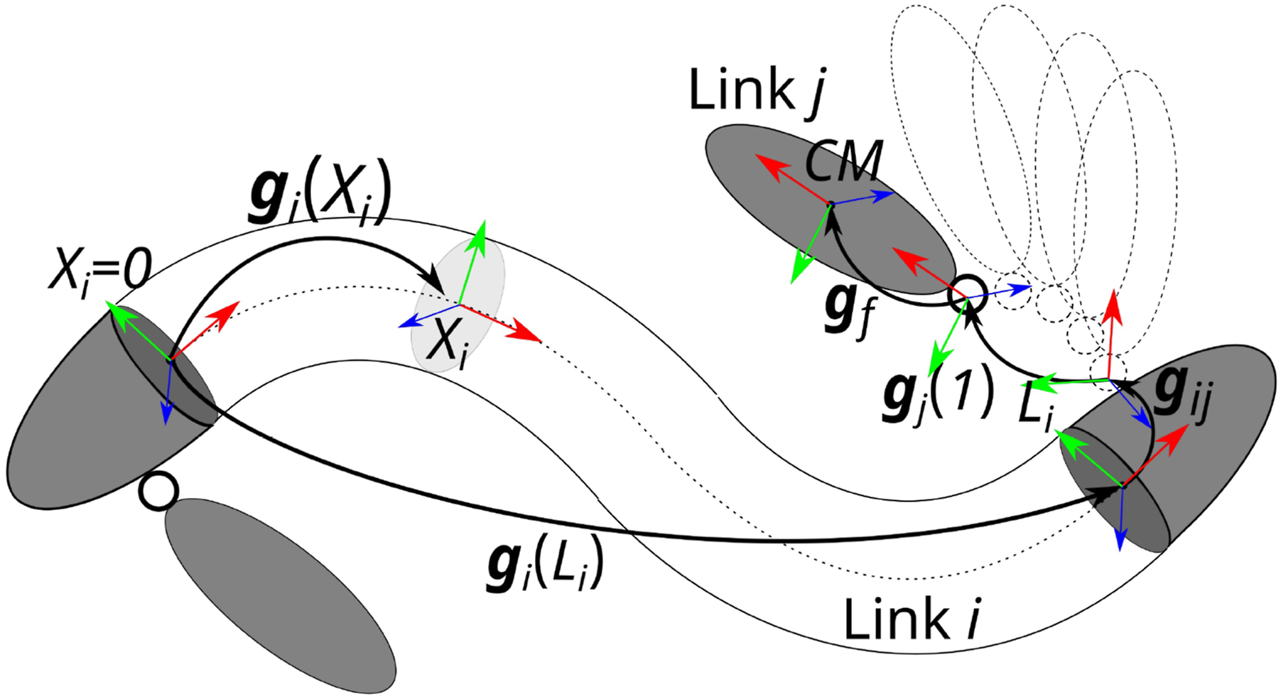g _ij and g _f are fixed transformations from i to j and rigid joint to the center of mass (CM) of the rigid link, respectively. The immaterial configurations of the rigid body are depicted as dashed shapes. Red, green, and blue arrows indicate the local x, y, and z axes, respectively.

2.1. Recursive kinematics

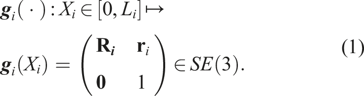
A floating hybrid kinematic chain is composed of interconnected rigid and soft bodies, here represented by Cosserat rods. The configuration of a soft body i (respectively, a rigid body) with respect to the body frame at its base is defined as a curve:

$\begin{array}{l}{\mathit{g}}_i(·):X_i\in \left[0,L_i\right]\mapsto \\ {\mathit{g}}_i\left(X_i\right)=\left(\begin{array}{ll}{\mathbf{R}}_{\mathit{i}}& {\mathbf{r}}_i\\ \mathbf{0}& 1\end{array}\right)\in SE\left(3\right).\end{array}$

(1)

note that, g _i ∈ SE(3) maps a point in the body-frame at X _i (curvilinear abscissa) to the body-frame at X _i = 0 ( g _i (0) = I ₄).

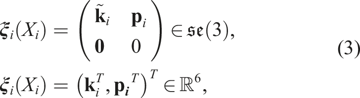
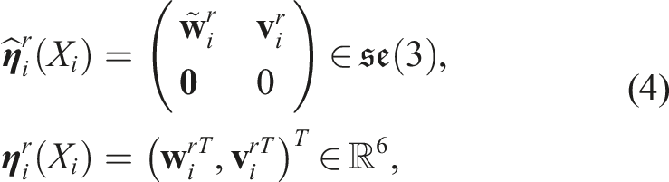
To study the exponential representation of (1), we introduce its partial derivatives with respect to X _i (indicated by (⋅)′) and time (indicated by $\stackrel{.}{(·)}$ ). We obtain

$\begin{array}{ll}{\mathit{g}}_i^{\prime }\left(X_i\right)& ={\mathit{g}}_i{\widehat{\mathit{\xi }}}_i,\end{array}$

(2a)

$\begin{array}{ll}{\dot{\mathit{g}}}_i\left(X_i\right)& ={\mathit{g}}_i{\widehat{\mathit{\eta }}}_i^{\mathit{r}},\end{array}$

(2b)

where

$\begin{array}{ll}{\widehat{\mathit{\xi }}}_i\left(X_i\right)& =\left(\begin{array}{ll}{\stackrel{\sim }{\mathbf{k}}}_i& {\mathbf{p}}_i\\ \mathbf{0}& 0\end{array}\right)\mathfrak{\in }\mathfrak{s}\mathfrak{e}\left(3\right),\\ {\mathit{\xi }}_i\left(X_i\right)& ={\left({\mathbf{k}}_i^T,{{\mathbf{p}}_{\mathit{i}}}^T\right)}^T\in {\mathbb{R}}^6,\end{array}$

(3)

defines the strain twist in body-frame, and

$\begin{array}{ll}{\widehat{\mathit{\eta }}}_i^r\left(X_i\right)& =\left(\begin{array}{ll}{\stackrel{\sim }{\mathbf{w}}}_i^r& {\mathbf{v}}_i^r\\ \mathbf{0}& 0\end{array}\right)\mathfrak{\in }\mathfrak{s}\mathfrak{e}\left(3\right),\\ {\mathit{\eta }}_i^r\left(X_i\right)& ={\left({\mathbf{w}}_i^{rT},{\mathbf{v}}_i^{rT}\right)}^T\in {\mathbb{R}}^6,\end{array}$

(4)

is the velocity twist relative to the previous body frame (here at X _i = 0) and expressed in the current body frame (here at X _i ). In (3), ${\stackrel{\sim }{\mathbf{k}}}_i\left(X_i\right)\mathfrak{\in }\mathfrak{s}\mathfrak{o}\left(3\right),{\mathbf{k}}_i\left(X_i\right)\in {\mathbb{R}}^3$ and ${\mathbf{p}}_i\left(X\right)\in {\mathbb{R}}^3$ are, respectively, the angular and linear strains. In (4), ${\stackrel{\sim }{\mathbf{w}}}_i^r\left(X_i\right)\mathfrak{\in }\mathfrak{s}\mathfrak{o}\left(3\right),{\mathbf{w}}_i^r\left(X_i\right)\in {\mathbb{R}}^3$ and ${\mathbf{v}}_i^r\left(X_i\right)\in {\mathbb{R}}^3$ are, respectively, the angular and linear velocities relative to the predecessor (superscript r).

The forward kinematics of a body ( g _i (X _i )) can be evaluated by the spatial integration of equation (2a). We first notice that the equation holds for both rigid and soft bodies, thanks to the following analogy. Imagine labeling the configuration of a rigid link i with a continuous independent variable X _i ∈ [0, 1] where X _i = 0 refers to the “initial” configuration, X _i = 1 points to the link body-frame “after” the joint motion and the rest indicates the intermediate poses. Thanks to this analogy, the “initial” (X _i = 0) configuration of the rigid link corresponds to the Cosserat rod’s base, while the “final” (X _i = 1) pose corresponds to the rod’s tip. Clearly, we are interested only in the “final” (X _i = 1) configuration in the rigid body case since the other frames are immaterial (Figure 1).

Now, the first of the equations in (2a) is a matrix differential equation that can be integrated in space. For the rigid link case, ${\widehat{\mathit{\xi }}}_i\left(X_i\right)$ is constant in X _i and equal to the body-frame representation of the joint twist attached to i. Thus, the integration provides:

${\mathit{g}}_i\left(1\right)=\exp \left({\widehat{\mathit{\xi }}}_i\right)$

(5)

The exponential map in SE(3) Selig (2007) is provided in Appendix A. For the soft link with constant strain ( ξ _i (X _i ) = ξ _i ), the integration of equation (2a) is straightforward and is addressed in the PCS model (Renda et al., 2018). However, in general ${\widehat{\mathit{\xi }}}_i\left(X_i\right)$ is variable in X _i . Hence, there is no closed solution for the integration. We need to employ the Magnus expansion (Hairer et al., 2006) of ξ _i at X _i given by Ω _i (X _i ), to apply the exponential map.

${\mathit{g}}_i\left(X_i\right)=\exp \left({\widehat{\mathbf{\Omega }}}_i\left(X_i\right)\right)$

(6)

Magnus expansion is an integral series of Lie Brackets of ${\widehat{\mathit{\xi }}}_i\left(X_i\right)$ . The Magnus expansion (Ω _i (X _i )) of the strain twist of a soft body (distributed joint) is equivalent to the joint twist ( ξ _i ) of a lumped joint. While, for a rigid body, we have ξ _i = Ω _i (1). Hence, equations (6) and (5) are identical by virtue of Magnus expansion. We use an approximate series of finite order to compute the Magnus expansion. A fourth-order Zannah quadrature approximation of Magnus expansion is provided in Appendix A.

Like any finite series, the Magnus expansion will degrade for larger values of X _i . Hence, the soft link shall be divided into smaller intervals of lengths h _j and g _i (X _i ) is evaluated recursively through these intervals:

${\mathit{g}}_i\left(X_i+h_j\right)={\mathit{g}}_i\left(X_i\right)\exp \left({\widehat{\mathbf{\Omega }}}_i\left(h_j\right)\right),$

(7)

note that g _i (0) = I. We will drop the subscript j of h _j to simplify subsequent equations. The recursion jumps from one point to the next as a rigid joint with a joint twist of Ω _i (h). Replacing g _i with ${{\mathit{g}}_i}_s$ in equation (7) we get the recursive formula for ${{\mathit{g}}_i}_s$ , which is configuration of link i with respect to the spatial frame (Figure 2(a)). The same formulation is applicable for rigid joints (Figure 2(b)).

$\begin{array}{ll}{{\mathit{g}}_i}_s\left(X_i+h\right)& ={{\mathit{g}}_i}_s\left(X_i\right)\exp \left({\widehat{\mathbf{\Omega }}}_i\left(h\right)\right),\end{array}$

(8a)

$\begin{array}{ll}{{\mathit{g}}_i}_s\left(1\right)& ={{\mathit{g}}_i}_s\left(0\right)\exp \left({\widehat{\mathit{\xi }}}_i\right),\end{array}$

(8b)

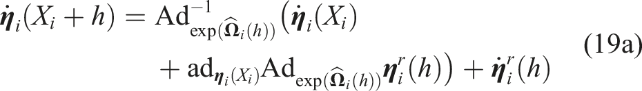
Figure 2.

Equivalence of soft links and rigid joints, by the virtue of Magnus expansion: (a) Shows the recursive progression from X _i to X _i + h for a soft link. (b) Shows the equivalent fictitious progression from X _i = 0 to X _i = 1 for a rigid joint (a prismatic joint used here).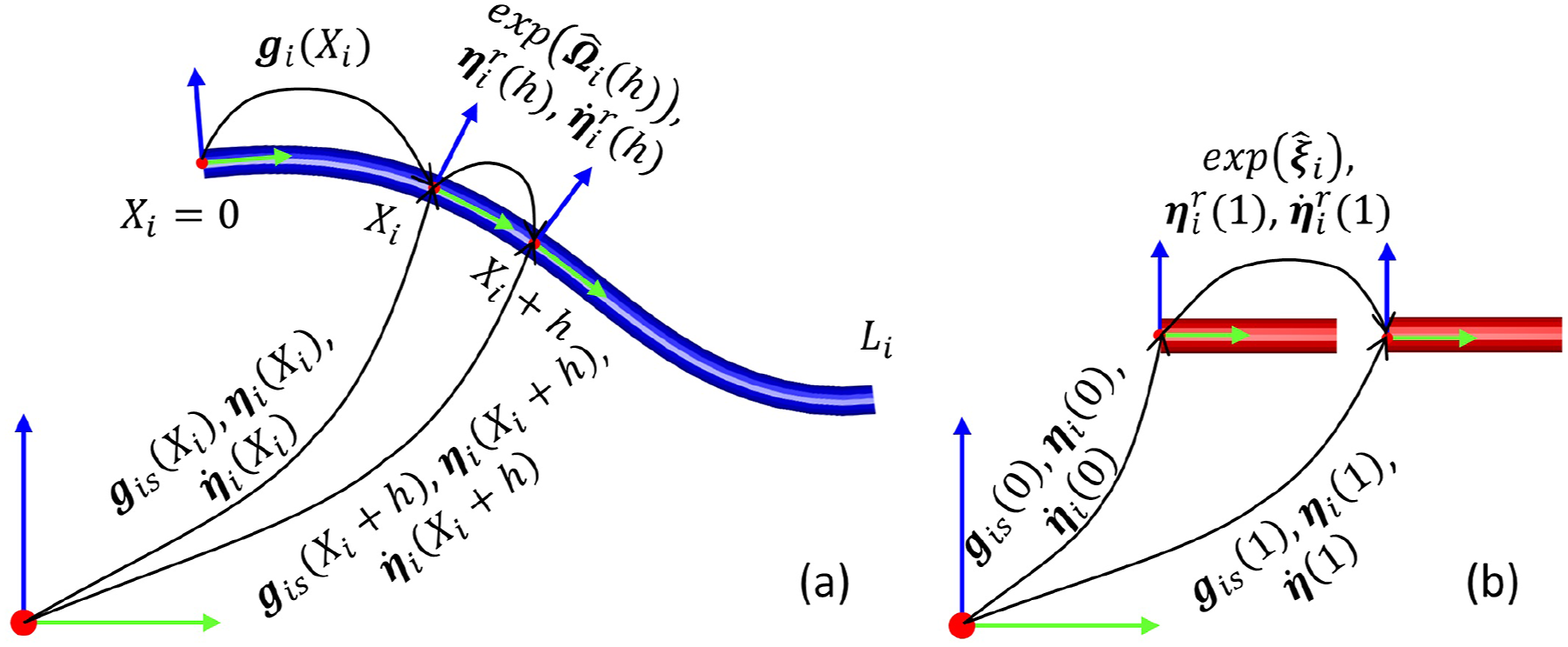

Next, we seek to find a relation between the time derivative of the strain twists and the links velocity and acceleration twist. Considering the equality of the mixed partial derivative of g _i , we obtain the space derivatives of relative velocity and acceleration twists (Boyer and Renda, 2017):

$\begin{array}{ll}{\mathit{\eta }}_i^{r^{\prime }}& ={\stackrel{.}{\mathit{\xi }}}_i-{\text{ad}}_{{\mathit{\xi }}_i}{\mathit{\eta }}_i^r,\end{array}$

(9)

$\begin{array}{ll}{\dot{\mathit{\eta }}}_i^{r^{\prime }}& ={\ddot{\mathit{\xi }}}_i-{\text{ad}}_{{\stackrel{.}{\mathit{\xi }}}_i}{\mathit{\eta }}_i^r-{\text{ad}}_{{\mathit{\xi }}_i}{\dot{\mathit{\eta }}}_i^r,\end{array}$

(10)

where ${\text{ad}}_{(·)}\in {\mathbb{R}}^{6\times 6}$ is the adjoint operator of $\mathfrak{s}\mathfrak{e}\left(3\right)$ (see Appendix A). By virtue of the identities ${\left({\text{Ad}}_{\mathit{g}}\right)}^{\prime }={\text{Ad}}_{\mathit{g}}{\text{ad}}_{\mathit{\xi }}$ , and $\stackrel{.}{\left({\text{Ad}}_{\mathit{g}}\right)}={\text{Ad}}_{\mathit{g}}{\text{ad}}_{{\mathit{\eta }}^r}$ (Section 8.3.1 in Lynch and Park (2017)), it can be verified that the analytic integration of (9) and (10) is given by

$\begin{array}{ll}{\mathit{\eta }}_i^r\left(X_i\right)& ={\text{Ad}}_{{\mathit{g}}_i}^{-1}{\int }_0^{X_i}{\text{Ad}}_{{\mathit{g}}_i}{\dot{\mathit{\xi }}}_{i}ds,\end{array}$

(11)

$\begin{array}{ll}{\dot{\mathit{\eta }}}_i^r\left(X_i\right)& ={\text{Ad}}_{{\mathit{g}}_i}^{-1}\left({\int }_0^{X_i}\left(\stackrel{.}{{\text{Ad}}_{{\mathit{g}}_i}}{\stackrel{.}{\mathit{\xi }}}_i+{\text{Ad}}_{{\mathit{g}}_i}{\ddot{\mathit{\xi }}}_i\right)ds\right),\end{array}$

(12)

where Ad_(·) is the adjoint map defined in Appendix A. Once again, equations (9)–(12) hold for both, rigid and soft links. For a rigid (multidimensional) joint, since ${\stackrel{.}{\mathit{\xi }}}_i$ and ${\ddot{\mathit{\xi }}}_i$ are constant in X _i , equations (11) and (12) can be integrated in space (X _i ∈ [0, 1]) to arrive at

$\begin{array}{ll}{\mathit{\eta }}_i^r\left(1\right)& ={\text{Ad}}_{\exp \left({\widehat{\mathit{\xi }}}_i\right)}^{-1}T\left({\mathit{\xi }}_i\right){\dot{\mathit{\xi }}}_i,\end{array}$

(13)

$\begin{array}{ll}{\dot{\mathit{\eta }}}_i^r\left(1\right)& ={\text{Ad}}_{\exp \left({\widehat{\mathit{\xi }}}_i\right)}^{-1}\left(\dot{T}\left({\mathit{\xi }}_i,{\stackrel{.}{\mathit{\xi }}}_i\right){\stackrel{.}{\mathit{\xi }}}_i+T\left({\mathit{\xi }}_i\right){\ddot{\mathit{\xi }}}_i\right),\end{array}$

(14)

where T and $\dot{T}$ are the tangent operator of the exponential map and its time derivative. Their analytical expressions are provided in Appendix A. It is worth noting that in the case of one-dimensional rigid joints, we have ${\text{Ad}}_{{\mathit{g}}_i}{\stackrel{.}{\mathit{\xi }}}_i={\stackrel{.}{\mathit{\xi }}}_i$ . Thus, equations (11) and (12) reduce to (Featherstone (2008))

${\mathit{\eta }}_i^r\left(1\right)={\dot{\mathit{\xi }}}_i,{\dot{\mathit{\eta }}}_i^r\left(1\right)={\ddot{\mathit{\xi }}}_i.$

(15)

Again, for a soft link, there is no explicit solution for the integration. Using the approximated Magnus expansion of ξ _i (X _i ) in an interval of h, equations (11) and (12) can be approximately evaluated as

$\begin{array}{ll}{\mathit{\eta }}_i^r\left(h\right)& ={\text{Ad}}_{\exp \left({\widehat{\mathbf{\Omega }}}_i\left(h\right)\right)}^{-1}T\left({\mathbf{\Omega }}_i\right){\stackrel{.}{\mathbf{\Omega }}}_i\left(h\right),\end{array}$

(16)

$\begin{array}{ll}{\dot{\mathit{\eta }}}_i^r\left(h\right)& ={\text{Ad}}_{\exp \left({\widehat{\mathbf{\Omega }}}_i\left(h\right)\right)}^{-1}\left(\dot{T}\left({\mathbf{\Omega }}_i,{\dot{\mathbf{\Omega }}}_i\right){\dot{\mathbf{\Omega }}}_i\left(h\right)+T\left({\mathbf{\Omega }}_i\right){\ddot{\mathbf{\Omega }}}_i\left(h\right)\right),\end{array}$

(17)

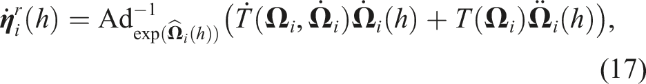
Note that here ${\mathit{\eta }}_i^r\left(h\right)$ and ${\dot{\mathit{\eta }}}_i^r\left(h\right)$ are velocity and acceleration twists of body frames at X _i + h relative to the previous body-frame at X _i . The equivalence between equations (13), (14) and (16), (17) brings the analysis of rigid joints and soft bodies (distributed joints) under the same framework. Similar to the computation of ${{\mathit{g}}_i}_s\left(X_i\text{or}1\right)$ , we can use a recursive scheme for the evaluation of absolute velocity twists or soft bodies or rigid joints in body-frame ( η _i (X _i or 1)):

$\begin{array}{ll}{\mathit{\eta }}_i\left(X_i+h\right)& ={\text{Ad}}_{\exp \left({\widehat{\mathbf{\Omega }}}_i\left(h\right)\right)}^{-1}{\mathit{\eta }}_i\left(X_i\right)+{\mathit{\eta }}_i^r\left(h\right),\end{array}$

(18a)

$\begin{array}{ll}{\mathit{\eta }}_i\left(1\right)& ={\text{Ad}}_{\exp \left({\widehat{\mathit{\xi }}}_i\right)}^{-1}{\mathit{\eta }}_i\left(0\right)+{\mathit{\eta }}_i^r\left(1\right),\end{array}$

(18b)

while their time derivative gives absolute acceleration twists:

${\stackrel{.}{\mathit{\eta }}}_i\left(X_i+h\right)={\text{Ad}}_{\exp \left({\widehat{\mathbf{\Omega }}}_i\left(h\right)\right)}^{-1}\left({\stackrel{.}{\mathit{\eta }}}_i\left(X_i\right)+{\text{ad}}_{{\mathit{\eta }}_i\left(X_i\right)}{\text{Ad}}_{\exp \left({\widehat{\mathbf{\Omega }}}_i\left(h\right)\right)}{\mathit{\eta }}_i^r\left(h\right)\right)+{\dot{\mathit{\eta }}}_i^r\left(h\right)$

(19a)

${\stackrel{.}{\mathit{\eta }}}_i\left(1\right)={\text{Ad}}_{\exp \left({\widehat{\mathit{\xi }}}_i\right)}^{-1}\left({\stackrel{.}{\mathit{\eta }}}_i\left(0\right)+{\text{ad}}_{{\mathit{\eta }}_i\left(0\right)}{\text{Ad}}_{\exp \left({\widehat{\mathit{\xi }}}_i\right)}{\mathit{\eta }}_i^r\left(1\right)\right)+{\dot{\mathit{\eta }}}_i^r\left(1\right)$

(19b)

Equations (8), (18), and (19) highlight the similarity of formulations of soft bodies and rigid joints. Finally, to pass from link “i” to “j,” which is rigidly connected to “i” with a fixed transformation matrix g _ij one can use

$\begin{array}{ll}{{\mathit{g}}_j}_s\left(0\right)& ={{\mathit{g}}_i}_s\left(L_i\text{or}1\right){\mathit{g}}_{ij},\end{array}$

(20a)

$\begin{array}{ll}{\mathit{\eta }}_j\left(0\right)& ={\text{Ad}}_{{\mathit{g}}_{ij}^{-1}}{\mathit{\eta }}_i\left(L_i\text{or}1\right),\end{array}$

(20b)

$\begin{array}{ll}\stackrel{.}{{\mathit{\eta }}_j}\left(0\right)& ={\text{Ad}}_{{\mathit{g}}_{ij}^{-1}}\stackrel{.}{{\mathit{\eta }}_i}\left(L_i\text{or}1\right)\end{array}$

(20c)

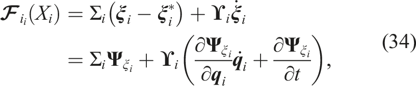
2.2. Strain parametrization

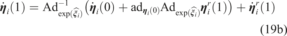
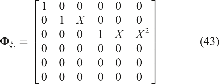
It is time now to discretize the system configuration (the strain) and introduce the generalized coordinates and basis functions. To this end, the continuous strain fields ξ _i are parametrized by a finite functional basis of strain modes.

${\mathit{\xi }}_i\left(X_i,{\mathit{q}}_i,t\right)={\mathbf{\Psi }}_{{\xi }_i}\left(X_i,{\mathit{q}}_i,t\right)+{\mathit{\xi }}_i^{\ast }\left(X_i\right),$

(21)

where ${\mathbf{\Psi }}_{{\mathit{\xi }}_i}\in {\mathbb{R}}^{6\times 1}$ is a general form for the strain field, which is a function of X _i , ${\mathit{q}}_i\in {\mathbb{R}}^{n_i}$ (vector of generalized coordinates of dimension n _i ) and t, which is the time. ${\mathit{\xi }}_i^{\ast }\in {\mathbb{R}}^6$ is a reference strain whose primary function is to model non-zero yet constrained strains such as inextensibility. The basis function $\left({\mathbf{\Psi }}_{{\xi }_i}\right)$ defines a function space, which can accurately model any strain fields that lie within this space. Strain fields that lie outside this space are not modeled by the basis function. Note that equation (21) is a general form of strain field which is typically expressed as a linear function of q (Renda et al. (2020)):

${\mathit{\xi }}_i\left(X_i,{\mathit{q}}_i\right)={\mathbf{\Phi }}_{{\xi }_i}\left(X_i\right){\mathit{q}}_i+{\mathit{\xi }}_i^{\ast }\left(X_i\right),$

(22)

In this case, ${\mathbf{\Phi }}_{{\mathit{\xi }}_i}\in {\mathbb{R}}^{6\times n_i}$ is independent of q _i and t and the function space is linearly spanned by ${\mathbf{\Phi }}_{{\xi }_i}$ . Note that the matrix ${\mathbf{\Phi }}_{{\mathit{\xi }}_i}\left(X_i\right)$ is constant for rigid joints: ${\mathit{\xi }}_i\left({\mathit{q}}_i\right)={\mathbf{\Phi }}_{{\xi }_i}{\mathit{q}}_i$ . For instance, for a revolute joint with an axis along the local x-axis, ${\mathbf{\Phi }}_{{\mathit{\xi }}_i}={\left[1,0,0,0,0,0\right]}^T$ .

The first and second time-derivatives of strain from equation (21) are given by

$\begin{array}{ll}\stackrel{.}{{\mathit{\xi }}_i}& =\frac{\partial {\mathbf{\Psi }}_{{\xi }_i}}{\partial {\mathit{q}}_i}\stackrel{.}{{\mathit{q}}_i}+\frac{\partial {\mathbf{\Psi }}_{{\xi }_i}}{\partial t},\end{array}$

(23)

$\begin{array}{ll}\ddot{{\mathit{\xi }}_i}& =\frac{\partial {\mathbf{\Psi }}_{{\xi }_i}}{\partial {\mathit{q}}_i}\ddot{{\mathit{q}}_i}+\left(\frac{{\partial }^2{\mathbf{\Psi }}_{{\xi }_i}}{\partial {{\mathit{q}}_i}^2}\stackrel{.}{{\mathit{q}}_i}+2\frac{{\partial }^2{\mathbf{\Psi }}_{{\xi }_i}}{\partial {\mathit{q}}_i\partial t}\right)\stackrel{.}{{\mathit{q}}_i}+\frac{{\partial }^2{\mathbf{\Psi }}_{{\xi }_i}}{{\partial }^{2}t},\end{array}$

(24)

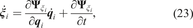
For independent bases (which are not functions of q _i and t) (equation (22)), we get

$\begin{array}{ll}\stackrel{.}{{\mathit{\xi }}_i}& ={\mathbf{\Phi }}_{{\xi }_i}\stackrel{.}{{\mathit{q}}_i}\end{array}$

(25)

$\begin{array}{ll}\ddot{{\mathit{\xi }}_i}& ={\mathbf{\Phi }}_{{\xi }_i}\ddot{{\mathit{q}}_i}\end{array}$

(26)

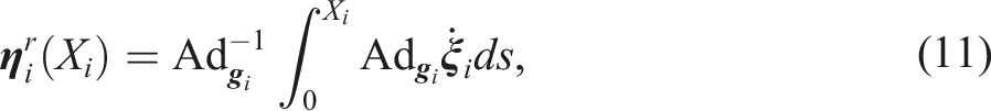
As mentioned earlier, the recursive computation of kinematics ( g _i (X _i )), velocity ( η _i (X _i )), acceleration $\left({\stackrel{.}{\mathit{\eta }}}_i\left(X_i\right)\right)$ twists involves the implementation of an approximated Magnus expansion. In the j ^th interval of material length h between two consecutive points, the Magnus expansion (Ω _i (h)) can be approximated at any order, following the Zanna collocation approach (Zanna, 1999). The detailed descriptions of computations of Ω _i (h), ${\stackrel{.}{\mathbf{\Omega }}}_i\left(h\right)$ , and ${\ddot{\mathbf{\Omega }}}_i\left(h\right)$ for a fourth-order approximation are provided in the Appendix A. Substituting those into equation (18) we get the recursive formula for absolute velocity in terms of generalized coordinates. From equation (23) it is easy to see that the velocity twist consists of two parts: due to the variation of generalized coordinates and time. The former produces a recursive formula for the geometric Jacobian while the second part leads to a velocity component solely due to the variation of time:

${\mathit{\eta }}_i\left(X_i,\mathit{q},\stackrel{.}{\mathit{q}},t\right)={\mathit{J}}_i\left(X_i,\mathit{q},t\right)\stackrel{.}{\mathit{q}}+{{\mathit{\eta }}_i}_t\left(X_i,\mathit{q},t\right)$

(27)

The recursive formula for ${\mathit{J}}_i\in {\mathbb{R}}^{6\times n_{\mathit{dof}}}$ and ${{\mathit{\eta }}_i}_t\in {\mathbb{R}}^{6\times 1}$ are provided in Appendix B. Note that here, $\mathit{q}\in {\mathbb{R}}^{n_{\mathit{dof}}}$ is the vector of n _dof generalized coordinates of the complete chain. The Jacobian for independent bases takes the same form of equation (27) without ${{\mathit{\eta }}_i}_t$ :

${\mathit{\eta }}_i\left(X_i,\mathit{q},\stackrel{.}{\mathit{q}}\right)={\mathit{J}}_i\left(X_i,\mathit{q}\right)\stackrel{.}{\mathit{q}}$

(28)

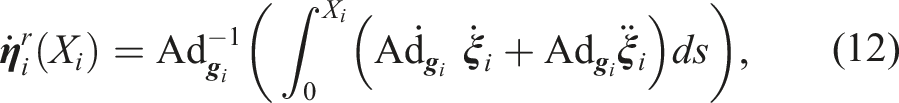
Similarly from equation (2.1), we can derive the absolute acceleration twist for dependent bases:

$\begin{array}{ll}{\stackrel{.}{\mathit{\eta }}}_i\left(X_i,\mathit{q},\stackrel{.}{\mathit{q}},\ddot{\mathit{q}},t\right)& ={\mathit{J}}_i\left(X_i,\mathit{q},t\right)\ddot{\mathit{q}}+{\mathit{Z}}_i\left(X_i,\mathit{q},\stackrel{.}{\mathit{q}},t\right)\stackrel{.}{\mathit{q}}\\ & +{{\mathit{\zeta }}_i}_t\left(X_i,\mathit{q},\stackrel{.}{\mathit{q}},t\right),\end{array}$

(29)

where,

$\begin{array}{ll}{\mathit{Z}}_i& ={\stackrel{.}{\mathit{J}}}_i+\frac{\partial {{\mathit{\eta }}_i}_t}{\partial {\mathit{q}}_i},\end{array}$

(30a)

$\begin{array}{ll}{{\mathit{\zeta }}_i}_t& =\frac{\partial {{\mathit{\eta }}_i}_t}{\partial t}\end{array}$

(30b)

For independent bases, the acceleration twist do not have ζ _it , while Z _i is equal to the derivative of the Jacobian:

${\stackrel{.}{\mathit{\eta }}}_i\left(X_i,\mathit{q},\stackrel{.}{\mathit{q}},\ddot{\mathit{q}}\right)={\mathit{J}}_i\left(X_i,\mathit{q}\right)\ddot{\mathit{q}}+{\stackrel{.}{\mathit{J}}}_i\left(X_i,\mathit{q},\stackrel{.}{\mathit{q}}\right)\stackrel{.}{\mathit{q}},$

(31)

The recursive formulas for ${\mathit{Z}}_i\in {\mathbb{R}}^{6\times n_{\mathit{dof}}}$ , ${{\mathit{\zeta }}_i}_t\in {\mathbb{R}}^{6\times 1}$ , and ${\stackrel{.}{\mathit{J}}}_i\in {\mathbb{R}}^{6\times n_{\mathit{dof}}}$ are provided in Appendix B. and Appendix C. Due to the analogy between the joint twist of a rigid joint ( ξ ) and the Magnus expansion of the strain twist (Ω(h)) of soft bodies, the equations of η _i and ${\stackrel{.}{\mathit{\eta }}}_i$ are equivalent for rigid joints.

2.3. Dynamics and statics

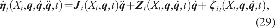
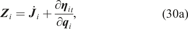
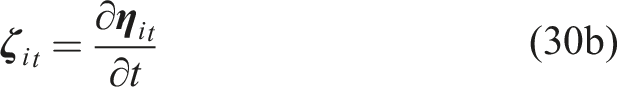
Once the Jacobian is found, the generalized dynamics of the floating hybrid chain can be obtained by projecting the free dynamics of each link by virtue of D’Alembert’s principle (Renda and Seneviratne, 2018). Note that the virtual displacement varies only with respect to q , not t. The free-body dynamic equations for a rigid link in the body-frame is (Murray et al. (1994))

${\mathcal{M}}_i{\stackrel{.}{\mathit{\eta }}}_i+{\text{ad}}_{{\mathit{\eta }}_i}^{\ast }{\mathcal{M}}_{\mathit{i}}{\mathit{\eta }}_i={\mathcal{F}}_{J_i}-{\displaystyle \sum }_j{\text{Ad}}_{{\mathit{g}}_{ij}{\mathit{g}}_j}^{\ast }{\mathcal{F}}_{J_j}+{\mathcal{F}}_{e_i}$

(32)

where ${\mathcal{M}}_i\in {\mathbb{R}}^{6\times 6}$ represents the screw inertia matrix ( ${\mathcal{M}}_i=\text{diag}\left(I_{x_i},I_{y_i},I_{z_i},m_i,m_i,m_i\right)$ if the body frame is a principal axis frame, m _i being the body mass and $I_{{·}_i}$ the second moment of inertia), ${\mathcal{F}}_{J_{(·)}}\in {\mathbb{R}}^6$ is the wrench transmitted across joint (⋅), ${\mathcal{F}}_{e_i}\in {\mathbb{R}}^6$ is the concentrated external load, while ${\text{ad}}_{(·)}^{\ast },{\text{Ad}}_{(·)}^{\ast }\in {\mathbb{R}}^{6\times 6}$ are the coadjoint operator and coadjoint map, respectively (see Appendix A).

For a soft link, the free-body dynamic equation in the local frame and its boundary conditions are given by the Cosserat equilibrium (Boyer and Renda (2017)):

$\begin{array}{l}{\overline{\mathcal{M}}}_i{\stackrel{.}{\mathit{\eta }}}_i+{\text{ad}}_{{\mathit{\eta }}_i}^{\ast }{\overline{\mathcal{M}}}_i{\mathit{\eta }}_i={\left({\mathcal{F}}_{i_i}-{\mathcal{F}}_{a_i}\right)}^{\prime }+{\text{ad}}_{{\mathit{\xi }}_i}^{\ast }\left({\mathcal{F}}_{i_i}-{\mathcal{F}}_{a_i}\right)+{\overline{\mathcal{F}}}_{e_i},\\ \left({\mathcal{F}}_{i_i}-{\mathcal{F}}_{a_i}\right)\left(0\right)=-{\mathcal{F}}_{J_i},\\ \left({\mathcal{F}}_{i_i}-{\mathcal{F}}_{a_i}\right)\left(L_i\right)=-{\displaystyle \sum }_j{\text{Ad}}_{{\mathit{g}}_{ij}}^{\ast }{\mathcal{F}}_{J_j}.\end{array}$

(33)

where ${\overline{\mathcal{M}}}_i\left(X_i\right)\in {\mathbb{R}}^{6\times 6}$ is the screw inertia density matrix of the cross-section ( ${\overline{\mathcal{M}}}_i={\rho }_i\text{diag}\left(J_{x_i},J_{y_i},J_{z_i},A_i,A_i,A_i\right)$ if the local frame is a principal axis frame, ρ _i being the mass density, A _i (X _i ) the cross-section area, and $J_{{·}_i}$ the second moment of area), ${\overline{\mathcal{F}}}_{e_i}\left(X_i\right)\in {\mathbb{R}}^6$ is the distributed external load, and ${\mathcal{F}}_{i_i}\left(X_i\right),{\mathcal{F}}_{a_i}\left(X_i\right)\in {\mathbb{R}}^6$ are the internal wrenches due to the material elasticity and distributed actuation, respectively. See Figure 3 for a graphical representation.

Figure 3.

Schematics of the dynamics of a soft link internally actuated.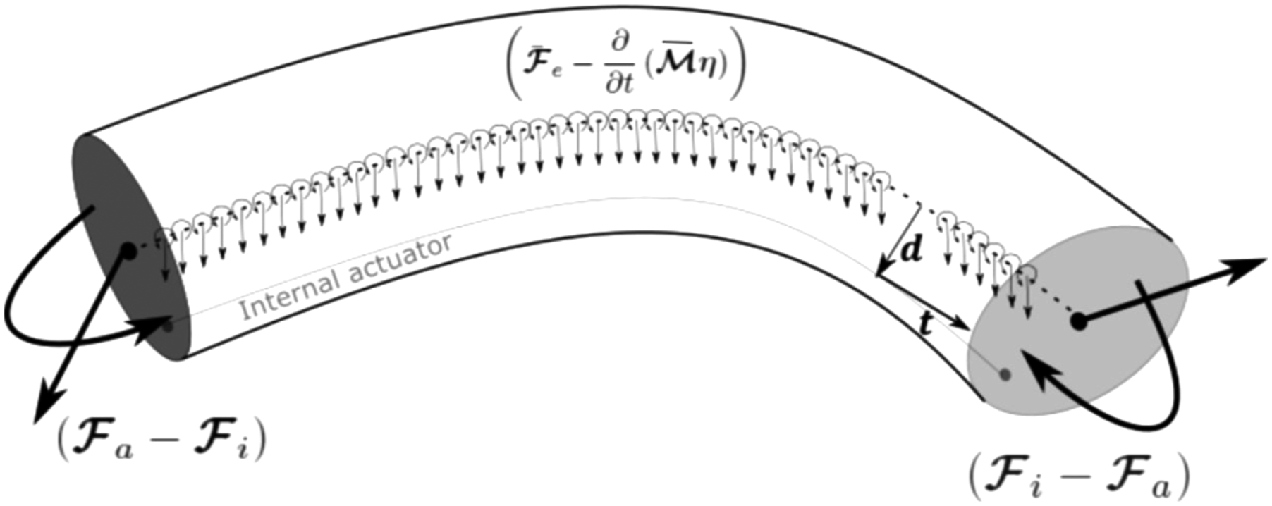

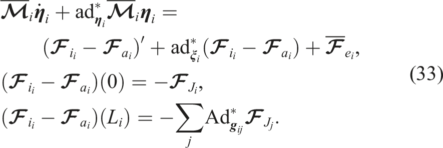
For what concerns the internal elastic wrench, ¹ one can take the derivative of any elastic energy potential that better describes the rod elasticity. Without loss of generality, for a Hook-like linear elastic law we get

$\begin{array}{l}{\mathcal{F}}_{i_i}\left(X_i\right)={\mathrm{\Sigma }}_i\left({\mathit{\xi }}_i-{\mathit{\xi }}_i^{\ast }\right)+{\mathbf{\Upsilon }}_i{\stackrel{.}{\mathit{\xi }}}_i\\ ={\mathrm{\Sigma }}_i{\mathbf{\Psi }}_{{\xi }_i}+{\mathbf{\Upsilon }}_i\left(\frac{\partial {\mathbf{\Psi }}_{{\xi }_i}}{\partial {\mathit{q}}_i}\stackrel{.}{{\mathit{q}}_i}+\frac{\partial {\mathbf{\Psi }}_{{\xi }_i}}{\partial t}\right),\end{array}$

(34)

where ${\mathrm{\Sigma }}_i\left(X_i\right)=\text{diag}\left(G_i{J}_{x_i},E_i{J}_{y_i},E_i{J}_{z_i},E_i{A}_i,G_i{A}_i,G_i{A}_i\right)\in {\mathbb{R}}^{6\times 6}$ is the screw elasticity matrix, E _i being the Young modulus and G _i the shear modulus (note that we have assumed the local x − axis to be perpendicular to the cross-section), and ${\mathbf{\Upsilon }}_i\left(X_i\right)=\upsilon \text{diag}\left(J_{x_i},3J_{y_i},3J_{z_i},3A_i,A_i,A_i\right)\in {\mathbb{R}}^{6\times 6}$ is the screw damping matrix, υ being the material damping. Note that the formulation allows non-linear and time-dependent elastic laws. One simply needs to replace equation (34) with appropriate constitutive law.

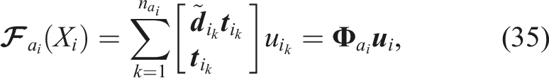
With regards to the actuation, in general, ${\mathcal{F}}_{a_i}$ can be any distributed actuation wrench. In some cases, it can be discretized using actuation bases. For example, consider thread-like actuators such as tendons and embedded pneumatic chambers (Renda et al., 2017). The actuation wrench is obtained by computing the force and moment exerted on the mid-line of the rod. This is given by (Renda et al. (2020)):

${\mathcal{F}}_{a_i}\left(X_i\right)={\displaystyle \sum }_{k=1}^{n_{a_i}}\left[\begin{array}{l}{\stackrel{\sim }{\mathit{d}}}_{i_k}{\mathit{t}}_{i_k}\\ {\mathit{t}}_{i_k}\end{array}\right]u_{i_k}={\mathbf{\Phi }}_{a_i}{\mathit{u}}_i,$

(35)

where ${\mathbf{\Phi }}_{a_i}\left({\mathit{q}}_i,X_i,t\right)\in {\mathbb{R}}^{6\times n_{a_i}}$ ( $n_{a_i}$ being the number of actuators of link i) is the actuation basis, ${\mathit{d}}_{i_k}\left(X_i\right)\in {\mathbb{R}}^3$ represents the distance from the mid-line to actuator k, ${\mathit{t}}_{i_k}\left({\mathit{q}}_i,X_i,t\right)\in {\mathbb{R}}^3$ is the unit vector tangent to the actuator path, and ${\mathit{u}}_i\in {\mathbb{R}}^{n_{a_i}}$ is the vector of magnitude actuation forces (see Figure 3).

It is now possible to obtain the generalized dynamic equation of the system via D’Alembert’s principle. We consider two cases, 1: with at least one dependent base and 2: where all bases are independent of q and t.

2.3.1. Case 1. Dependent bases

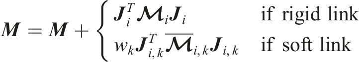
Substituting equations (27) and (29) into (32) and (33) projecting them onto the space of generalized coordinates through the Jacobians J _i and integrating over the length of the soft links yields

$\mathit{M}\ddot{\mathit{q}}+\mathit{C}\stackrel{.}{\mathit{q}}+{\mathit{C}}_1+{\mathit{K}}_1+{\mathit{D}}_1=\mathit{B}\mathit{u}+\mathit{F},$

(36)

where $\mathit{M}\left(\mathit{q},t\right)\in {\mathbb{R}}^{n_{\mathit{dof}}\times n_{\mathit{dof}}}$ is the generalized mass matrix, $\mathit{C}\left(\mathit{q},\stackrel{.}{\mathit{q}},t\right)\in {\mathbb{R}}^{n_{\mathit{dof}}\times n_{\mathit{dof}}}$ is the generalized Coriolis matrix, ${\mathit{C}}_1\left(\mathit{q},\stackrel{.}{\mathit{q}},t\right)\in {\mathbb{R}}^{n_{\mathit{dof}}}$ is a generalized force component due to the presence of time-dependent bases, ${\mathit{D}}_1\left(\mathit{q},\stackrel{.}{\mathit{q}},t\right)\in {\mathbb{R}}^{n_{\mathit{dof}}}$ is the generalized damping force, ${\mathit{K}}_1\left(\mathit{q},t\right)\in {\mathbb{R}}^{n_{\mathit{dof}}}$ is the generalized elastic force, $\mathit{B}\left(\mathit{q},t\right)\in {\mathbb{R}}^{n_{\mathit{dof}}\times n_a}$ (n _a being the total number of actuators) is the generalized actuation matrix, $\mathit{F}\left(\mathit{q},\stackrel{.}{\mathit{q}},t\right)\in {\mathbb{R}}^{n_{\mathit{dof}}}$ is the vector of generalized external forces and $\mathit{u}\left(t\right)\in {\mathbb{R}}^{n_a}$ is the vector of applied actuation forces. These components are detailed below.

$\mathit{M}\left(\mathit{q},t\right)={\displaystyle \sum }_{i=1}^N{\int }_0^{L_i}{\mathit{J}}_i^T\overline{\mathcal{M}}{\mathit{J}}_{i}d{X}_i$

(37a)

$\mathit{C}\left(\mathit{q},\stackrel{.}{\mathit{q}},t\right)={\displaystyle \sum }_{i=1}^N{\int }_0^{L_i}{\mathit{J}}_i^T\left({\text{ad}}_{{\mathit{\eta }}_i}^{*}\overline{\mathcal{M}}{\mathit{J}}_i+\overline{\mathcal{M}}{\mathit{Z}}_i\right)d{X}_i$

(37b)

${\mathit{C}}_1\left(\mathit{q},\stackrel{.}{\mathit{q}},t\right)={\displaystyle \sum }_{i=1}^N{\int }_0^{L_i}{\mathit{J}}_i^T\left({\text{ad}}_{{\mathit{\eta }}_i}^{*}\overline{\mathcal{M}}{\mathit{\eta }}_{it}+\overline{\mathcal{M}}{\mathit{\zeta }}_{it}\right)d{X}_i$

(37c)

${{\mathit{D}}_1\left(\mathit{q},\stackrel{.}{\mathit{q}},t\right)=\Vert }_{i=1}^N\left({\int }_0^{L_i}{\left(\frac{\partial {\mathbf{\Psi }}_{{\xi }_i}}{\partial {\mathit{q}}_i}\right)}^T{\mathbf{\Upsilon }}_i{\stackrel{.}{\mathit{\xi }}}_{i}d{X}_i\right)$

(37d)

${{\mathit{K}}_1\left(\mathit{q},t\right)=\Vert }_{i=1}^N\left({\int }_0^{L_i}{\left(\frac{\partial {\mathbf{\Psi }}_{{\xi }_i}}{\partial {\mathit{q}}_i}\right)}^T{\mathbf{\Sigma }}_i{\mathbf{\Psi }}_{{\mathit{\xi }}_i}d{X}_i\right)$

(37e)

${\mathit{B}\left(\mathit{q},t\right)=\Vert }_{i=1}^N\left({\int }_0^{L_i}{\left(\frac{\partial {\mathbf{\Psi }}_{{\xi }_i}}{\partial {\mathit{q}}_i}\right)}^T{\mathbf{\Phi }}_{a_i}d{X}_i\right)$

(37f)

$\mathit{F}\left(\mathit{q},\stackrel{.}{\mathit{q}},t\right)={\displaystyle \sum }_{i=1}^N{\int }_0^{L_i}{\mathit{J}}_i^T{\overline{\mathcal{F}}}_{e_i}d{X}_i$

(37g)

where N is the total number of links and ‖ is the vertical concatenation operator. The components of (36) specified above are given from a soft link point of view. However, it is easy to recover the rigid body case by removing the integrals and replacing the distributed quantities with their lumped counterparts. Also, note that in the rigid link case the term Bu should be replaced with τ , which is the generalized joint wrench. The static equilibrium equation of the system can be derived from equation (36) by equating all time-derivatives to zero:

${\mathit{K}}_1=\mathit{B}\mathit{u}+\mathit{F}$

(38)

For more information on the mathematical procedure, we refer the reader to Renda et al. (2018), Renda and Seneviratne (2018), and Renda et al. (2020). For closed-chain systems, one may follow the approach recently presented in Armanini et al. (2021) to include the closed-loop constraints. The process involves the introduction of constrain forces into the generalized dynamics and the additional constrain equations expressed in the Pfaffian form (velocity level). For statics, the constraints are expressed in the position level.

2.3.2. Case 2. Independent bases

Similarly, using equations (28) and (31), we get the generalized dynamics and static equilibrium equations of a robot, which is modeled using independent bases:

$\begin{array}{ll}\mathit{M}\ddot{\mathit{q}}+\left(\mathit{C}+\mathit{D}\right)\stackrel{.}{\mathit{q}}+\mathit{K}\mathit{q}& =\mathit{B}\mathit{u}+\mathit{F},\end{array}$

(39a)

$\begin{array}{ll}\mathit{K}\mathit{q}& =\mathit{B}\mathit{u}+\mathit{F},\end{array}$

(39b)

where, in this case, $\mathit{D}\in {\mathbb{R}}^{n_{dof}\times n_{dof}}$ is the generalized damping matrix, $\mathit{K}\in {\mathbb{R}}^{n_{dof}\times n_{dof}}$ is the generalized stiffness matrix of the system.

$\mathit{D}={\text{diag}}_{i=0}^N\left({\int }_0^{L_i}{\mathbf{\Phi }}_{{\mathit{\xi }}_i}^T{\mathbf{\Upsilon }}_i{\mathbf{\Phi }}_{{\mathit{\xi }}_i}d{X}_i\right)$

(40a)

$\mathit{K}={\text{diag}}_{i=0}^N\left({\int }_0^{L_i}{\mathbf{\Phi }}_{{\mathit{\xi }}_i}^T{\mathbf{\Sigma }}_i{\mathbf{\Phi }}_{{\mathit{\xi }}_i}d{X}_i\right)$

(40b)

Note that D and K are constant for a chain modeled using independent bases and linear elastic materials. Hence they can be pre-computed before the static or dynamic analyses. Also note that, for independent bases, M , C , and B are not functions of time, the term C ₁ does not appear in the dynamics equation, Z _i is replaced with ${\stackrel{.}{\mathit{J}}}_i$ , and $\partial {\mathbf{\Psi }}_{{\xi }_i}/\partial {\mathit{q}}_i$ with ${\mathbf{\Phi }}_{{\mathit{\xi }}_i}$ . Readers may refer to Appendix C for their explicit formulas.

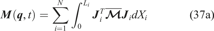
2.4. Computation

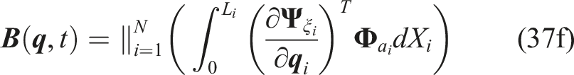
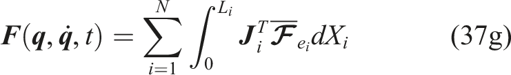
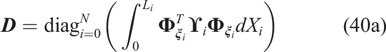
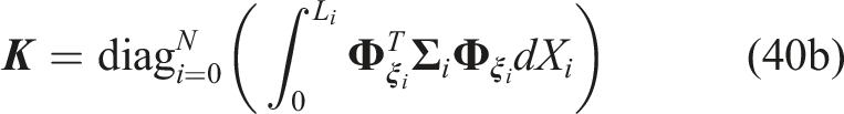
The dynamic analysis involves the temporal evolution of the system states, q (t) and $\stackrel{.}{\mathit{q}}\left(t\right)$ , and the static analysis involves the computation of the equilibrium state of the system. ODEs (36) or (39a) are numerically integrated for the former, while non-linear equation (38) or (39b) are numerically solved for the latter. The computation of components of these generalized equations requires the spatial integration of distributed quantities of soft links.

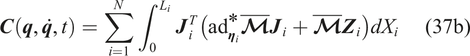
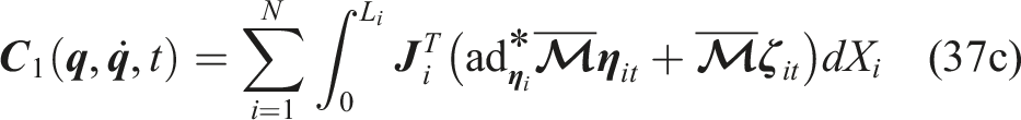
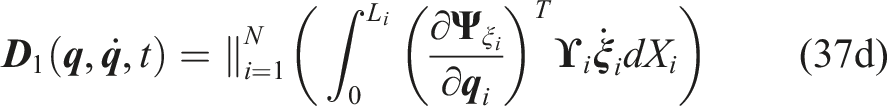
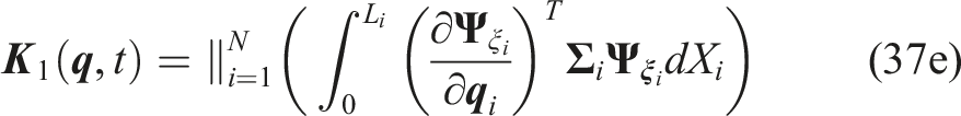
The spatial integrals in equation (37) or (40) can be evaluated using any numerical integration schemes like Gaussian-Legendre quadrature, which numerically evaluates the integrands at discrete points. This numerical integration method can be expressed as

${\int }_0^{L_i}\mathit{f}\left(X\right)dX={\displaystyle \sum }_{k=1}^{n_i}{w}_k\mathit{f}\left(X_k\right)$

(41)

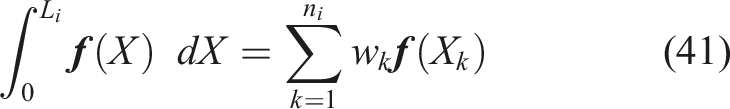
where n _i is the number of integration points, w _k are the quadrature weights, and X _k are the integration points (both scaled according to the integral limits). For instance, the roots of the n ^th order Legendre polynomial are used as the integration points for the Gauss quadrature method. Thus, a two-level nested quadrature scheme is used to get the generalized equations: Zannah collocation to evaluate the approximate Magnus expansion of the strain twist and the numerical scheme for the integration of (37) or (40). This resembles the orthogonal collocation method of Orekhov and Simaan Orekhov and Simaan (2020). Figure 4 provides a graphical representation of the numerical scheme for a single soft link with a three-point Gauss quadrature scheme as an example.

Figure 4.

Graphical representation of the two-level nested quadrature scheme for a soft link i. In this particular example, a three points Gauss quadrature (fourth-order) scheme is used for the integration, and a 2 point Zanna’s collocation method (fourth-order) is used for calculating the Magnus expansion.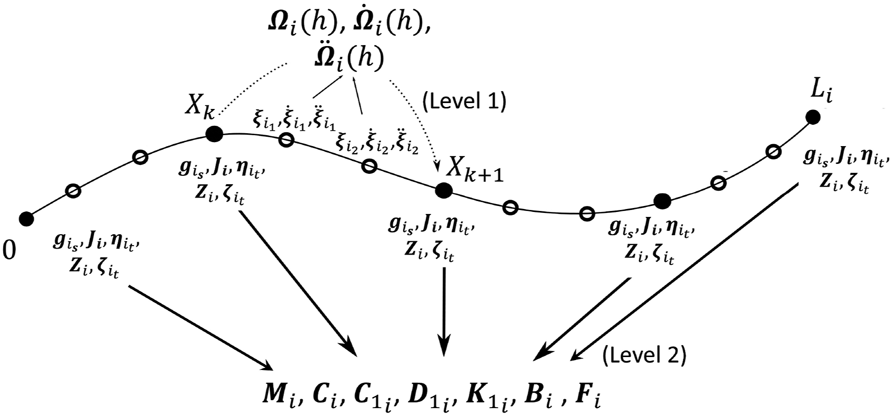

The Gauss quadrature integration scheme with n _G points gives an exact solution for the integration of a polynomial of order up to 2n _G − 1. For basis functions that cannot be approximated as polynomials, one should use a different integration scheme (e.g., trapezoidal quadrature, Simpson’s rule) that is compatible with the basis. The type of basis, the complexity of geometry, material models, external force, and actuation models must be considered while choosing the integration scheme and the number of points. In the following sections, the reader can find details of the integration scheme used for different bases.

For the computation of soft links, we propose a normalization scheme. We scale the domain of the i ^th link from [0, L _i ] m to [0, 1] units. Subsequently, all physical quantities of the link with length dimensions are converted into a new unit of length given by: L _i m = 1 unit. We perform all computations of the link using this new unit of length. This means the generalized coordinates of a soft link are expressed in the link’s unit of length. Finally, the projected free dynamics of the link is scaled back to m for computing the components of generalized dynamics or statics equation. Normalization has the following advantages: (i) All basis can be expressed as a function of X = X _i /L _i , the numerical value of the scaled curvilinear abscissa. (ii) All spatial integrations can be performed from 0 to 1 irrespective of the length of the soft link. (iii) All matrices (for instance, the generalized stiffness matrix) are scaled appropriately for a soft robot with multiple soft links. Properly scaled matrices are preferred for the speed and stability of numerical computations.

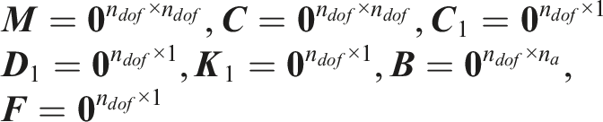
The computation for the dynamic analysis of the hybrid linkage can be simplified into the following steps:

Step 1: Computation of the system’s state and their derivatives ( q , $\stackrel{.}{\mathit{q}}$ ) at a given t (from Step 5). At t = 0, initial conditions are given.

Step 2: Initialization of components of generalized dynamics equation:

$\begin{array}{l}\mathit{M}={\mathbf{0}}^{n_{dof}\times n_{dof}},\mathit{C}={\mathbf{0}}^{n_{dof}\times n_{dof}},{\mathit{C}}_1={\mathbf{0}}^{n_{dof}\times 1}\\ {\mathit{D}}_1={\mathbf{0}}^{n_{dof}\times 1},{\mathit{K}}_1={\mathbf{0}}^{n_{dof}\times 1},\mathit{B}={\mathbf{0}}^{n_{dof}\times n_a},\\ \mathit{F}={\mathbf{0}}^{n_{dof}\times 1}\end{array}$

• Step 3: Recursive computation of g _i , J _i , ${{\mathit{\eta }}_i}_t$ , Z _i , and ${{\mathit{\zeta }}_i}_t$ at every computational points.

• Step 4: Incremental update of components of generalized dynamics equation at each computational point (center of mass of rigid links and space integration quadrature points for the soft links).

$\mathit{Q}=\mathit{Q}+\{\begin{array}{ll}{\mathit{Q}}_i& \text{if} \text{rigid} \text{link}\\ w_k{\overline{\mathit{Q}}}_{i,k}& \text{if} \text{soft} \text{link}\end{array},$

• where, Q represents the components of the generalized dynamics equation and Q _i or ${\overline{\mathit{Q}}}_{i,k}$ represent the contribution of i ^th rigid or soft link obtained from equation (37) (integrands). The subscript k represents the quantities evaluated at X _k . For instance, in the case of the generalized mass matrix,

$\mathit{M}=\mathit{M}+\{\begin{array}{ll}{\mathit{J}}_i^T{\mathcal{M}}_i{\mathit{J}}_i& \text{if} \text{rigid} \text{link}\\ w_k{\mathit{J}}_{i,k}^T{\overline{\mathcal{M}}}_{i,k}{\mathit{J}}_{i,k}& \text{if} \text{soft} \text{link}\end{array}$

• Step 5: Solve for $\ddot{\mathit{q}}$

$\ddot{\mathit{q}}={\mathit{M}}^{-1}\left(\mathit{B}\mathit{u}+\mathit{F}-\mathit{C}\stackrel{.}{\mathit{q}}-{\mathit{C}}_1-{\mathit{K}}_1-{\mathit{D}}_1\right)$

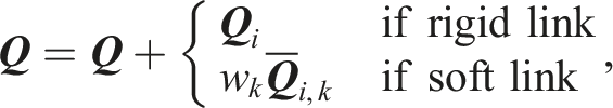
Steps 3 and 4 are repeated for all links. Note that for soft links, the computational point refers to their integration points, while for rigid links, typically, the center of mass is considered. As previously mentioned, closed-chain systems have additional constraint equations. We employ an explicit numerical integration scheme (like ode45 or ode15s of MATLAB) to propagate the computed value of $\ddot{\mathit{q}}$ at step 5 and evaluate the state (step 1) at the next time step. The integration proceeds until the specified time limit and generates the temporal evolution of q (t) and $\stackrel{.}{\mathit{q}}\left(t\right)$ . The static equilibrium analysis also follows a similar algorithm. We implemented these algorithms in the SoRoSim toolbox. We used the toolbox to perform all the static and dynamic analyses presented in this paper. Readers interested in the validation of the model for static and dynamic simulations are encouraged to refer to our previous paper on the SoRoSim Toolbox (Mathew et al., 2022a). Note that only independent global bases are used there.

3. Independent bases

Let us start our analysis with bases that are independent of q _i and t, given by equation (22). The most immediate advantage of independent bases over dependent ones is that their numerical values can be pre-computed and saved at all required points on the soft link $\left({\mathbf{\Phi }}_{{\mathit{\xi }}_i}\left(X\right)\right)$ . Then, for a given point, the screw strain and its derivatives can be computed as linear functions of q _i , ${\stackrel{.}{\mathit{q}}}_i$ , and ${\ddot{\mathit{q}}}_i$ using equations (22), (25), and (26). The generalized dynamics and static equilibrium equations are notably simpler for a floating hybrid chain (linkage) modeled completely using independent bases.

Independent base is an 6 × n _i matrix function of X ∈ [0, 1], whose columns are linearly independent vector functions. The k ^th column is typically defined as

${\left({\mathbf{\Phi }}_{{\xi }_i}\right)}_k={\left[{\mathbf{0}}_{m^{-}}{f}_k\left(X\right){\mathbf{0}}_{m^{+}}\right]}^T$

(42)

the equation implies that the k ^th component of q _i (q _k ) contributes only to the m ^th component of strain (m ∈ {1, 2, …, 6}). Note that equation (42) suggests that the strain components are decoupled with respect to q _k . However, this is not the most general definition of ${\left({\mathbf{\Phi }}_{{\xi }_i}\right)}_k$ . In a general case, q _k can contribute to more than one component of the strain twist.

The function f _k can span the entire domain of X or a smaller subdomain. The former type is classified as global shape functions, while the latter is called local shape functions. This section explores the properties of global and local strain bases, which are constructed using global and local shape functions. We also present three examples to highlight their applications.

3.1. Global bases

Global bases are constructed using global shape functions, which span the entire domain of an i ^th link, the value of strain at a given point depends on all elements of q _i . In other words, each element of q _i affects the whole domain of X. The most basic example of a global base is the one that is constructed using monomials, where the n ^th order monomial is given by: p _n (X) = X ⁿ (Figure 5(a)). For example, consider a monomial basis, which models a constant torsional strain about the local x-axis, linear bending about the y-axis, and quadratic bending z-axis:

${\mathbf{\Phi }}_{{\xi }_i}=\left[\begin{array}{llllll}1& 0& 0& 0& 0& 0\\ 0& 1& X& 0& 0& 0\\ 0& 0& 0& 1& X& X^2\\ 0& 0& 0& 0& 0& 0\\ 0& 0& 0& 0& 0& 0\\ 0& 0& 0& 0& 0& 0\end{array}\right]$

(43)

Figure 5.

Global basis functions which span the domain: (a) Monomial and (b) Legendre polynomial bases.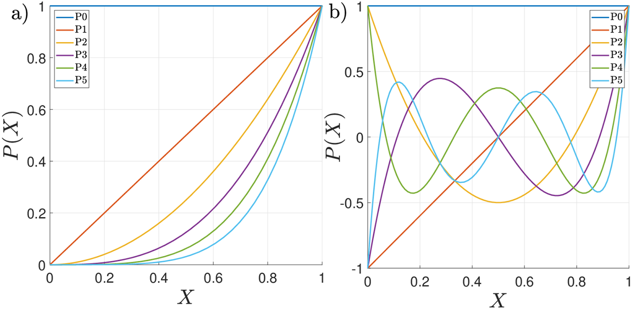

In this case, ${\mathit{q}}_i={\left[q_1,q_2,q_3,q_4,q_5,q_6\right]}^T$ , where q₁ is the constant torsional strain, q₂ and q₃ are constant and linear component of bending strain about the y-axis and so on. Note that, as the order increases, the difference between p _n and p_n+1 reduces significantly for monomial basis (Figure 5(a)). This may result in numerical errors for higher orders. There are other polynomial bases where this is not the case. Replacing X ⁿ with a Legendre polynomial of n ^th order, we get a Legendre polynomial basis. Figure 5(b) shows the graphical representation of Legendre basis functions. Note that Legendre polynomials are orthogonal under the inner product, ${\int }_0^1{p}_m\left(X\right)p_n\left(X\right)dX$ . Hence, if the screw elasticity (Σ _i ) and damping (ϒ _i ) matrices are constant, equation (40) suggests that K and D are diagonal.

Since monomials and Legendre polynomials are polynomial functions, in most cases, we can use a Gauss quadrature integration scheme of an appropriate number of integration points (n _G ) to compute the coefficients of generalized dynamics and static equilibrium equation (39), according to equation (41). The higher the value of n _G , the better the accuracy of the integral. However, the computational costs will be higher too. If the integrands in equation (37) (their independent equivalents) or (40) require a very high order polynomial to approximate, it is better to use an alternate quadrature scheme for their integration.

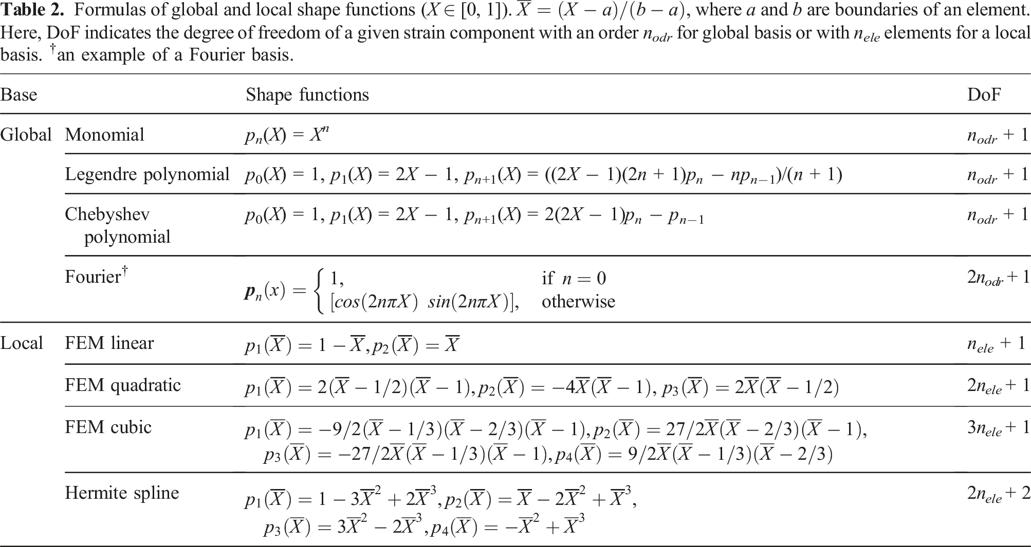
Various global bases based on different basis functions, such as Chebyshev’s polynomials and Fourier series, can be implemented according to the problem specifications. For instance, the Fourier basis is ideal to approximate strains that are periodic in X _i . Table 2 provides more details on these.

3.2. Local bases

A soft link may be subjected to local loads such as contact, point force, or boundary loads, which can introduce localized deformations. Local bases, where the generalized coordinates affect only a subdomain X _i , can be employed in such cases. Local bases are constructed using local shape functions.

We employed FEM-like bases, which divide a soft link into elements. While traditional FEM shape functions are used to describe the position field, we use them to model the strain field. The shape function can be linear, quadratic, or cubic, with 2, 3, and 4 nodes, respectively. Finally, at the shared point between two elements, we have a common node, which ensures strain continuity. Figure 6(a)–(c) describe the shape functions on a three-element soft link. The value of generalized coordinates corresponds to the value of strains at every node. Hence, they have an explicit physical meaning. Note that this particular type of strain parameterization makes it relative nodal reduction. Depending on the problem specifications, one can allow particular modes of strain out of the six possible modes. For FEM-like bases to model different degrees of freedom for different strain modes, we must create corresponding element grids for each mode with a different DoF. Also, the minimum DoF per strain mode is two, three, and four for linear, quadratic, and cubic types. It is worth noting that, for FEM bases, the generalized stiffness and damping matrices are band matrices (tri-, penta-, and hepta-diagonal for linear, quadratic, and cubic types) which is computationally preferable.

Figure 6.

Shape functions for a three-element soft link. Local bases: (a) Linear, (b) Quadratic, (c) Cubic FEM, and (d) Hermite spline bases. Each color corresponds to a strain mode that is governed by a single coordinate. The vertical dashed lines indicate the boundaries of each element, while the black dots indicate the location of the nodes, where the generalized coordinates are defined.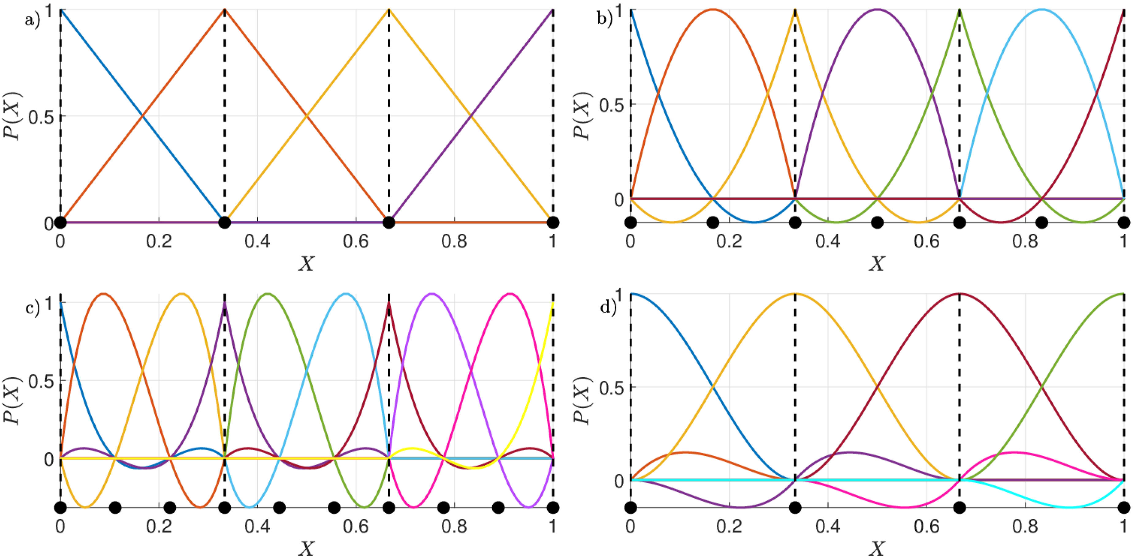

Since the shape functions are not polynomials that span the entire rod domain, we cannot use the Gauss quadrature scheme for the integration. We use elementwise integration—that is, we use a Gauss quadrature scheme on each element with their weights tuned according to the element’s length. A linear element requires at least two quadrature points for integration, while a quadratic or cubic element requires 3 and 4 points, respectively.

To demonstrate the concept of the local base, consider a fixed-free cylindrical beam with the parameters shown in Table 1. The beam is subjected to gravity, and the resulting static equilibrium configuration is solved. We compared two cases. The first case used a global base composed of the first 5 Legendre polynomials, resulting in n _dof = 5. The second case used a two-element quadratic shape function base, also resulting in n _dof = 5. In both cases, only the bending about the local y-axis was modeled. A five-point Gauss quadrature scheme was used for the first case, while the second case uses three quadrature points per element. The resulting strain field comparison can be seen in Figure 7(a). We used the same bases to analyze a scenario with an additional concentrated force of 30 N applied at X = 0.5 and oriented along the global x-axis. The resulting equilibrium strain fields are shown in 7b. As GroundTruth, we used commercial finite element software where the beam was discretized using 1000 linear elements. It can be observed that the local base solution accurately captured the local event occurring at the element boundary, where the global base solution deteriorates (Figure 7(b)). However, under the distributed load of gravity alone, the global base showed a better match to the reference solution. The local base solution introduced a non-justified jump in strain derivative at the element boundary.

Table 1.

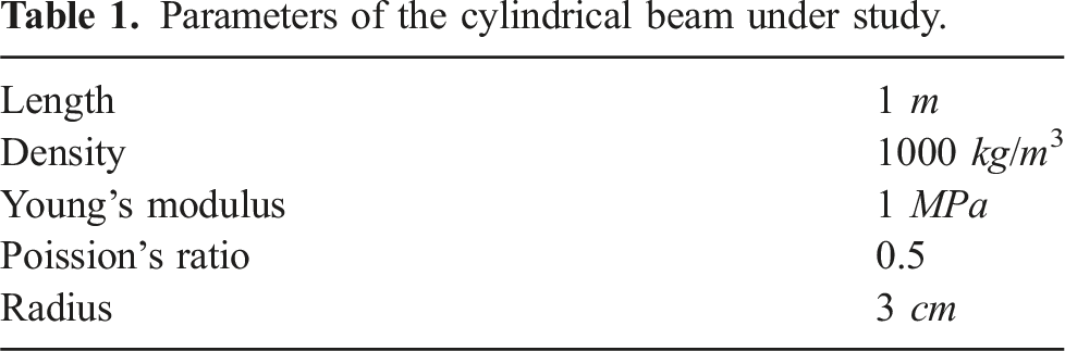
Parameters of the cylindrical beam under study.

Length	1 m
Density	1000 kg/m3
Young’s modulus	1 MPa
Poission’s ratio	0.5
Radius	3 cm

Figure 7.

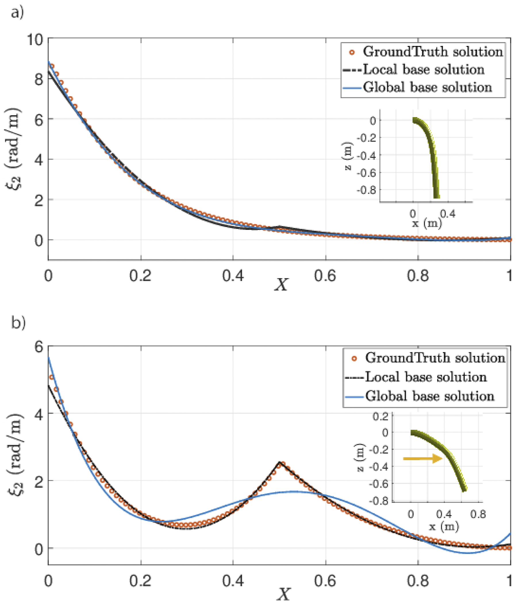
(a) Strain fields for the static equilibrium of a slender cylindrical beam under gravity using global and local bases. (b) Solution when applying a point force at X = 0.5.

We introduce an additional scenario to illustrate how global and local bases respond to perturbation. We solve the static equilibrium for an internally actuated arm using two different formulations: the first employs a fourth-order Legendre polynomial to characterize the bending strain, and the second utilizes a two-element quadratic FEM basis. Both approaches yield a system with five DoFs. We perturb the second coordinate of both static equilibrium solutions with a predefined percentage of perturbation. The impact of this perturbation is depicted in Figure 8. The global basis solution exhibits a substantial difference in the strain field and configuration due to the perturbation, illustrating the sensitivity of the solution. Conversely, the local basis displays a localized discrepancy in the strain field, and consequently a lower discrepancy in the configuration. These findings indicate that while global bases can efficiently capture complex fields with fewer DoFs, their susceptibility to perturbations could significantly alter the solution outcome. A complete sensitivity analysis requires an analytical derivative of the dynamic model, whih is beyond the scope of this paper. However, with some additional effort, it can be adapted from the rigid robotics literature (Sohl and Bobrow, 2001).

Figure 8.

Strain fields and configurations of the static equilibrium solutions in comparison to the perturbed ones for (a) global basis and (b) local basis.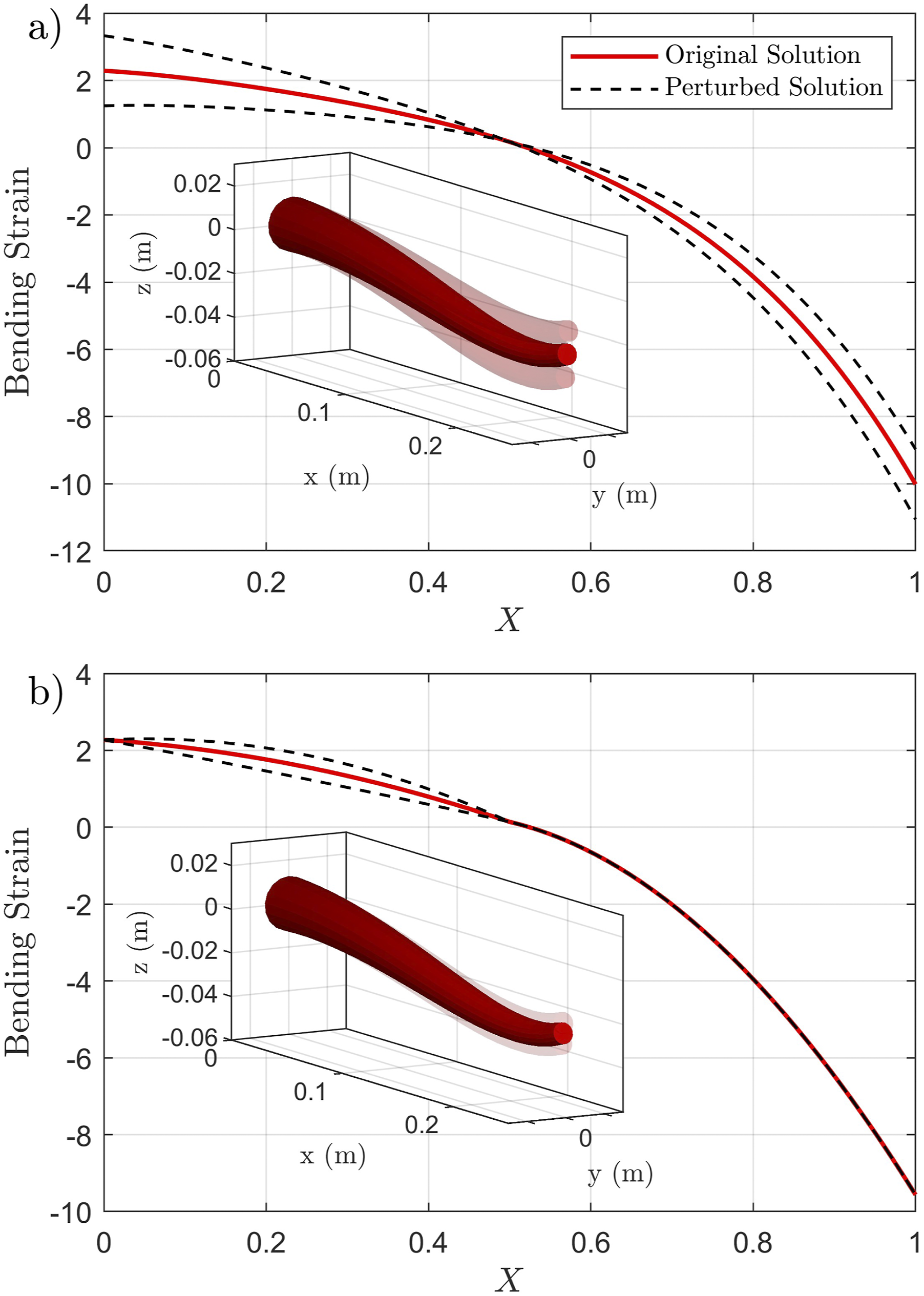

FEM-like bases are not the only possible local basis functions. We can construct local bases using any set of local shape functions. Another example is Hermite shape functions (cubic Hermite spline) which are C1 continuous (differentiable) at element boundaries. That is, the screw strain at element boundaries can be modeled as differentiable functions. In this case, the value of generalized coordinates corresponds to the value of strains and their space derivative at every node. Figure 6(d) shows the Hermite shape functions of a three-element soft link. Not that local bases essentially make the modeling a relative nodal reduction, while for a global basis, the same framework becomes a relative modal reduction (Armanini et al., 2023). Table 2 provides formulas of a few global and local shape functions, which can be used to construct corresponding strain bases.

Table 2.

Formulas of global and local shape functions (X ∈ [0, 1]). $\overline{X}=\left(X-a\right)/\left(b-a\right)$ , where a and b are boundaries of an element. Here, DoF indicates the degree of freedom of a given strain component with an order n _odr for global basis or with n _ele elements for a local basis. ^†an example of a Fourier basis.

Base		Shape functions	DoF
Global	Monomial	p n (X) = X n	n odr + 1
	Legendre polynomial	p0(X) = 1, p1(X) = 2X − 1, pn+1(X) = ((2X − 1)(2n + 1)p n − npn−1)/(n + 1)	n odr + 1
	Chebyshev polynomial	p0(X) = 1, p1(X) = 2X − 1, pn+1(X) = 2(2X − 1)p n − pn−1	n odr + 1
	Fourier†	${\mathit{p}}_n\left(x\right)=\{\begin{array}{ll}1,& \text{if} n=0\\ \left[\mathit{cos}\left(2n\pi X\right)\mathit{sin}\left(2n\pi X\right)\right],& \text{otherwise}\end{array}$	2n odr + 1
Local	FEM linear	$p_1\left(\overline{X}\right)=1-\overline{X},p_2\left(\overline{X}\right)=\overline{X}$	n ele + 1
	FEM quadratic	$p_1\left(\overline{X}\right)=2\left(\overline{X}-1/2\right)\left(\overline{X}-1\right),p_2\left(\overline{X}\right)=-4\overline{X}\left(\overline{X}-1\right)$ , $p_3\left(\overline{X}\right)=2\overline{X}\left(\overline{X}-1/2\right)$	2n ele + 1
	FEM cubic	$p_1\left(\overline{X}\right)=-9/2\left(\overline{X}-1/3\right)\left(\overline{X}-2/3\right)\left(\overline{X}-1\right),p_2\left(\overline{X}\right)=27/2\overline{X}\left(\overline{X}-2/3\right)\left(\overline{X}-1\right)$ , $p_3\left(\overline{X}\right)=-27/2\overline{X}\left(\overline{X}-1/3\right)\left(\overline{X}-1\right),p_4\left(\overline{X}\right)=9/2\overline{X}\left(\overline{X}-1/3\right)\left(\overline{X}-2/3\right)$	3n ele + 1
	Hermite spline	$p_1\left(\overline{X}\right)=1-3{\overline{X}}^2+2{\overline{X}}^3,p_2\left(\overline{X}\right)=\overline{X}-2{\overline{X}}^2+{\overline{X}}^3$ , $p_3\left(\overline{X}\right)=3{\overline{X}}^2-2{\overline{X}}^3,p_4\left(\overline{X}\right)=-{\overline{X}}^2+{\overline{X}}^3$	2n ele + 2

4. Dependent bases

Independent bases can model strains which are non-linear functions of X. However, they are linear with respect to q (subscript “i” is dropped in this section) and independent of time. Depending on the problem definition, it is possible to reduce the strain order by using strain bases that are non-linear in q and are dependent on t. Such bases are advantageous for order reduction especially when the strain field does not conform to a polynomial shape. A time-dependent basis can be employed when we have prior information regarding the temporal evolution of the strain field, such as the position of a concentrated load or the velocity of a traveling wave. Dependent bases take the most general form of strain presented in equation (21) where the strain can be a non-linear function of X, q , and t.

This section introduces dependent bases and explores their order reduction capabilities using two illustrative examples: (1) dependent bases that are functions of q and t and (2) dependent bases that are functions only of q . In both examples, we consider a slender beam of a length 0.8 m with a constant circular cross-section of diameter 3 cm, Young’s modulus of 1 MPa, Poisson’s ratio 0.5, and a material damping coefficient of 10⁴ Pa.s.

4.1. Basis dependent on q and t

We simulate the case where an internal actuation force, ${\overline{\mathcal{F}}}_a\left(X\right)={\left[0,M_2\left(X\right),0,0,0,0\right]}^T$ , is applied to the beam at a localized subdomain. The internal actuation moment, M₂(X), is modeled as a traveling triangular pulse in X, spanning 10% the length of the beam and traveling from the base to the tip in t _f seconds. To analyze this case, we define a strain basis as a non-linear Gaussian function of q and t:

$\mathbf{\Psi }\left(X,\mathit{q},t\right)={\left[0,q_1·e^{-q_2^2{\left(X-t/t_f\right)}^2},0,0,0,0\right]}^T,$

(44)

where $\mathit{q}={\left[q_1,q_2\right]}^T$ , where q₁ represents the maximum magnitude of the strain and q₂ is related to the standard deviation of the strain distribution. Note that equation (44) takes the most general form of the strain field given by equation (21). Our choice of Gaussian function as the basis is justified by the relatively accurate representation of the strain produced by internal moment actuation applied to a particular point. Figure 9 shows the static equilibrium of the system when the internal moment was applied at the midpoint of the beam (t/t _f = 0.5). The analytical solution can be obtained by solving the equation, ${\mathcal{F}}_i={\mathcal{F}}_a$ . The figure compares the solutions of 10 ^th (11 DoF) order monomial basis, Legendre polynomial basis, and the Gaussian dependent basis with the analytical solution. It is easy to see that the Gaussian basis performs better in terms of accuracy and order reduction. The Gaussian form of the strain basis cannot be approximated as a polynomial. Therefore, the Gauss quadrature scheme is not a viable option for integration. Instead, we used a trapezoidal integration scheme with 101 quadrature points. Throughout this paper, we employed the same integration scheme for all problems analyzed using dependent bases.

Figure 9.

Comparison of static equilibrium solutions when the internal moment M₂(X) is applied at the midpoint of the beam. The deformed shape of the body, corresponding to the analytical solution, is shown in the inset.

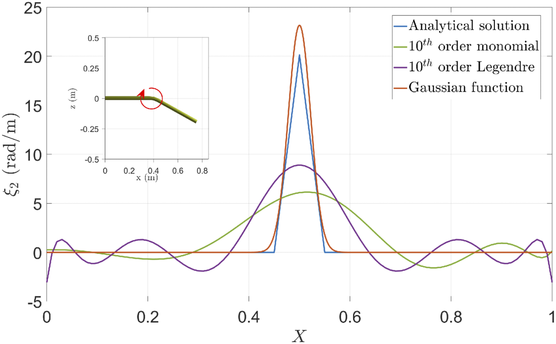
We now proceed with the dynamic simulation. The internal actuation moment is applied at X = (t/t _f ) with a constant peak magnitude of 0.5Nm (Figure 11(a)). The value of t _f is chosen as 2 s. Figure 11(a) and (b) show the dynamic strain distribution and the deformed shape of the beam. The dynamic simulation does not capture the transient response (strains) that lie outside of the finite function space of the proposed Gaussian basis function. To underscore this fact, we employed a Cubic FEM basis with 10 elements and compared the solution with that of the dependent basis. Noticeable differences exist in the solutions, especially in the part outside the Gaussian basis function. To enhance the representation of the system dynamics, additional basis functions could be integrated with the Gaussian basis. A detailed discussion of such a scenario is presented in Section 5.4. To gain a more comprehensive understanding of dynamic simulations presented in this article, we recommend the reader refer to the supplementary video. The simulation with dependent bases took 3 min and 10 s to complete using the ode15s integrator of MATLAB. The specifications of the PC which we used for the computations in this paper are as follows: Intel(R) Core(TM) i7-1065G7 CPU @ 1.30 GHz 1.50 GHz, 16.0 GB RAM. The MATLAB version we used for these analyses is R2020a.

4.2. Basis dependent on q

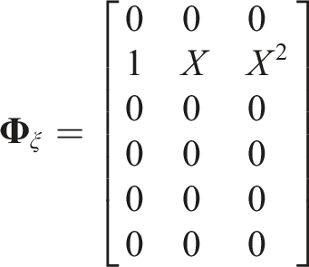
In our second example, we simulate the case where an external moment ${\overline{\mathcal{F}}}_e\left(X\right)={\left[0,M_2\left(X\right),M_3\left(X\right),0,0,0\right]}^T$ is applied to the beam. The distribution of the moments is again represented by a triangle pulse centered at a point and with a base width of 10% the length of the beam. In this case, we use a strain basis, which is a function of q but not a function of t. We define a Sigmoid basis function:

$\mathbf{\Psi }\left(X,\mathit{q}\right)={\left[0,\frac{q_1·e^{-q_2\left(X-q_3\right)}}{e^{-q_2\left(X-q_3\right)}+1},\frac{q_4·e^{-q_5\left(X-q_6\right)}}{e^{-q_5\left(X-q_6\right)}+1},0,0,0\right]}^T,$

(45)

where $\mathit{q}={\left[q_1,q_2,q_3,q_4,q_5,q_6\right]}^T$ , where q₁ and q₄ are related to the magnitude of the strain, q₂ and q₅ represent the slope of transition of the strain, and q₃ and q₆ represent the transition point. The Sigmoid function was chosen based on the form of the strain produced by an external moment applied at a particular point. Figure 10 shows the static equilibrium distribution of the strain on the beam when a moment, ${M_2}_{peak}=1Nm$ and M₃(X) = 0Nm, is applied at the midpoint of the beam. The analytical solution, in this case, can be obtained by solving, ${\mathcal{F}}_i^{\prime }+{\text{ad}}_{\mathit{\xi }}^{*}{\mathcal{F}}_i=-{\overline{\mathcal{F}}}_e$ . The figure provides a comparison between the solutions of the monomial basis of 10 ^th order, the Legendre polynomial basis of 10 ^th order, and the dependent Sigmoid function. The improvement in terms of accuracy and order reduction of the Sigmoid function is evident in this case.

Figure 10.

Comparison of static equilibrium solutions when the external moment M₂(X) is applied at the midpoint of the beam. The deformed shape of the body, corresponding to the analytical solution, is shown as an inset.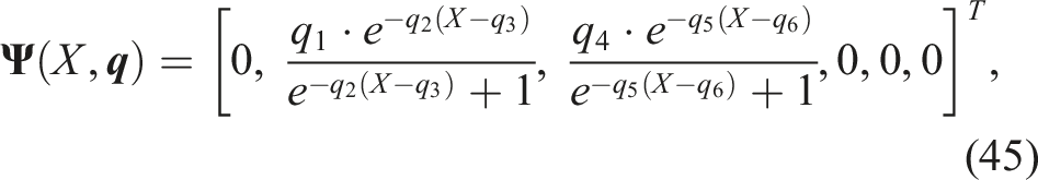

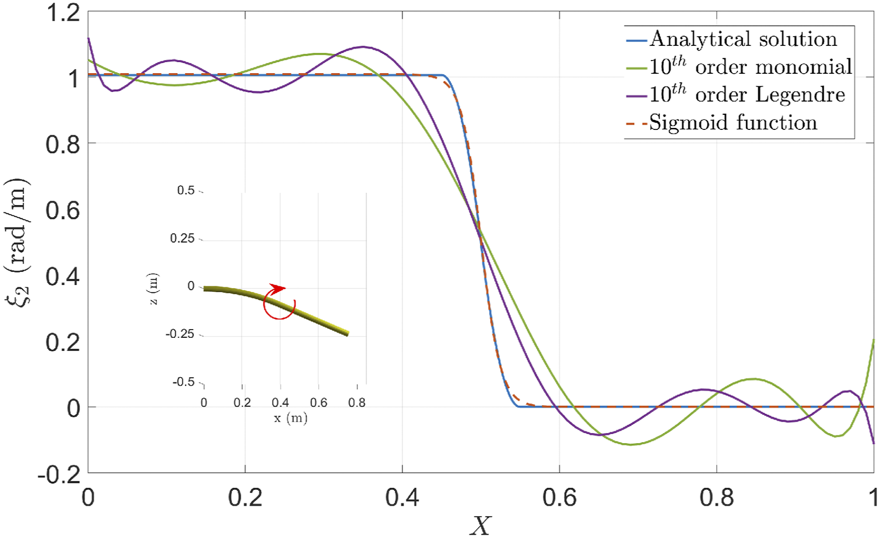
For the dynamics simulation, we linearly (in time) varied the location of the external moment from L/4 to 3 L/4. The magnitude of ${M_2}_{peak}$ is decreased over time from 4 Nm to 2 Nm whereas the ${M_3}_{peak}$ is increased from 4 Nm to 6 Nm. Figures 11(c) and (d) show the strains and the deformed shape of the beam for a simulation of 5 s. Even though the moments are linearly varied over time, the strain distribution does not follow the same trend. The transition point shifts along the location of the moment. However, the magnitude of the strain does not follow. This is particularly evident from the distribution of ξ ₃ (Figure 11(c)). We conclude that this is due to the dynamic response of the system. Note that, again, in this case, the transient behavior of the system, which is not modeled by the Sigmoid basis function, is not captured. The computational time for the simulation is 2 min and 11 s (ode15s integrator is used).

Figure 11.

Dynamic analysis using dependent bases: (a) Internal actuation moments and their corresponding dynamic strain distribution that is modeled using a time-dependent Gaussian basis function (solid line) and using FEM Cubic basis function (dashed line). (b) Superimposed snapshots of corresponding deformed shapes (dependent base). (c) External moments and their corresponding dynamic strain distributions that are modeled as Sigmoid functions. (d) Superimposed snapshots of corresponding deformed shapes.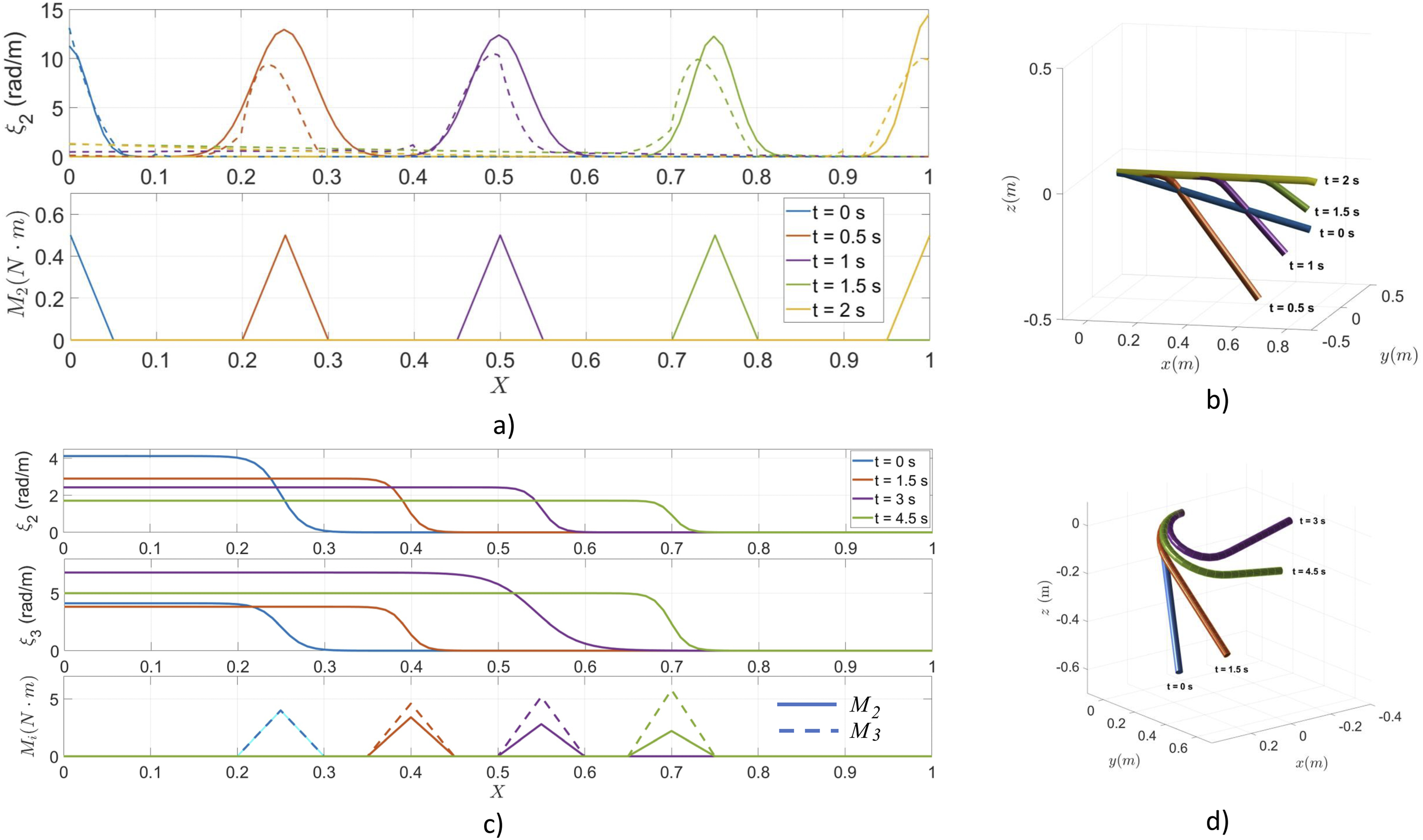

5. Applications

In this section, we explore the applications of the GVS model and the bases introduced in the previous sections. We consider four real-world scenarios for dynamic analysis. The first three scenarios focus on independent bases, while the last one combines both dependent and independent bases. The readers may refer to the supplementary video for the dynamic simulation results presented in this section.

5.1. Dynamics of a cable-driven soft manipulator

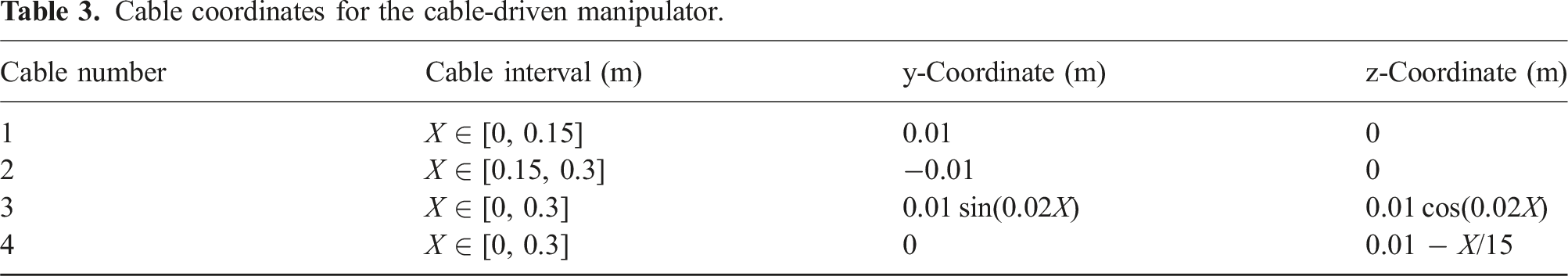
Tendon or cable-driven actuation is one of the most common actuation methods used in soft robotics. Pulling the cables that are embedded in the soft robot allows the introduction of actuation forces and moments that deform the robot. By tuning the actuator paths, the manipulators can achieve complex deformed shapes (Renda et al., 2020). Here we showcase a soft manipulator with four independent actuators as shown in Figure 12(a). We define the manipulator as a 30 cm cylindrical beam of 3 cm diameter, with a Young’s modulus of 1 MPa, a density of 1000 kg/m³ and a material damping coefficient of 10⁴ Pa.s. We subject the manipulator to gravitational load in the negative global Z direction. To define the actuator paths, we divide the manipulator into two sections of 15 cm each. The local y and z coordinates of the actuators are detailed in Table 3. The basis for the actuation is calculated using equation (35), using the actuators’ coordinates that are detailed in the Table.

Figure 12.

(a) Initial configuration and actuator paths, (b) Actuation profile for each of the four actuators, and (c) Snapshots of the cable-driven manipulator at different times. The red dots represent the trace of the manipulator’s tip.

Table 3.

Cable coordinates for the cable-driven manipulator.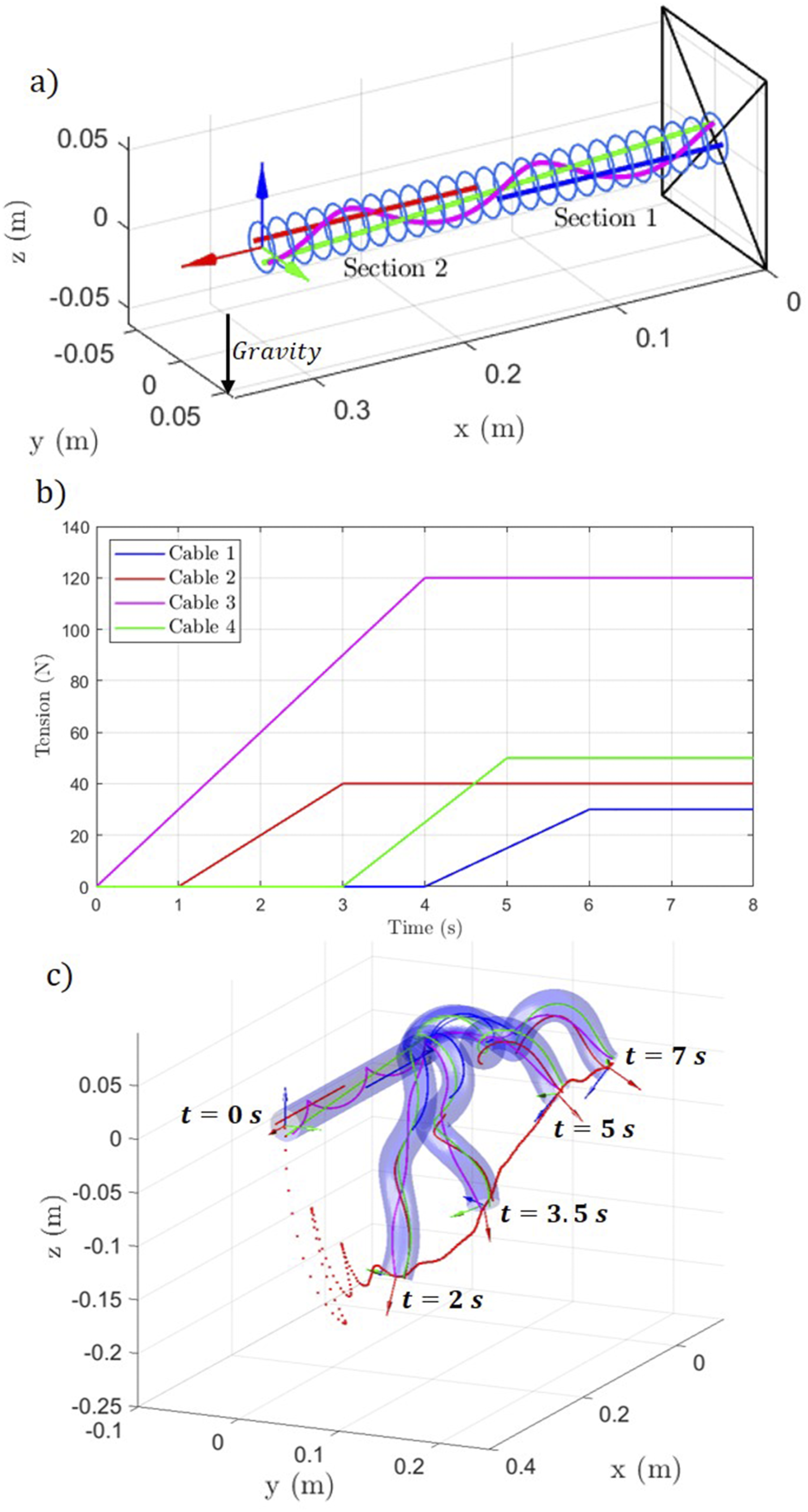

Cable number	Cable interval (m)	y-Coordinate (m)	z-Coordinate (m)
1	X ∈ [0, 0.15]	0.01	0
2	X ∈ [0.15, 0.3]	−0.01	0
3	X ∈ [0, 0.3]	0.01 sin(0.02X)	0.01 cos(0.02X)
4	X ∈ [0, 0.3]	0	0.01 − X/15

Discontinuity in the actuator path along the robot’s length introduces a discontinuity in the strain field. To capture this strain discontinuity, we divide the robot’s domain into two sections. Note that this approach is theoretically and computationally identical to employing discontinuous strain bases that take the value of zero on selected parts of the robot’s domain. We used a fourth-order Legendre polynomial basis for discretizing the torsional and bending (about y and z axes) strains. This results in 15 DoF for each section of the manipulator (a total of 30 DoF). We actuated the manipulator according to the cable tension profile shown in Figure 12(b) and computed the dynamic response of the system for the first 8 s. The resulting dynamic configurations of the manipulator at different time instants are shown in Figure 12(c). The complex transient behavior of the manipulator due to the combined effect of gravity, actuation forces, and material elasticity can be appreciated from the Figure.

To compare the computational performance, we simulate the same scenario again using a two-element quadratic FEM basis for each section of the manipulator, making the total DoF equal for both cases. For the spatial integration of each section of the manipulator, a five-point Gauss quadrature scheme was used for the global basis, while for the local basis, we used three Gauss quadrature points per element. The simulation time for the analysis using the global Legendre basis is 14.8 s, while the analysis using the local FEM took 18.2 s.

5.2. Locomotion and docking of an underwater soft robot

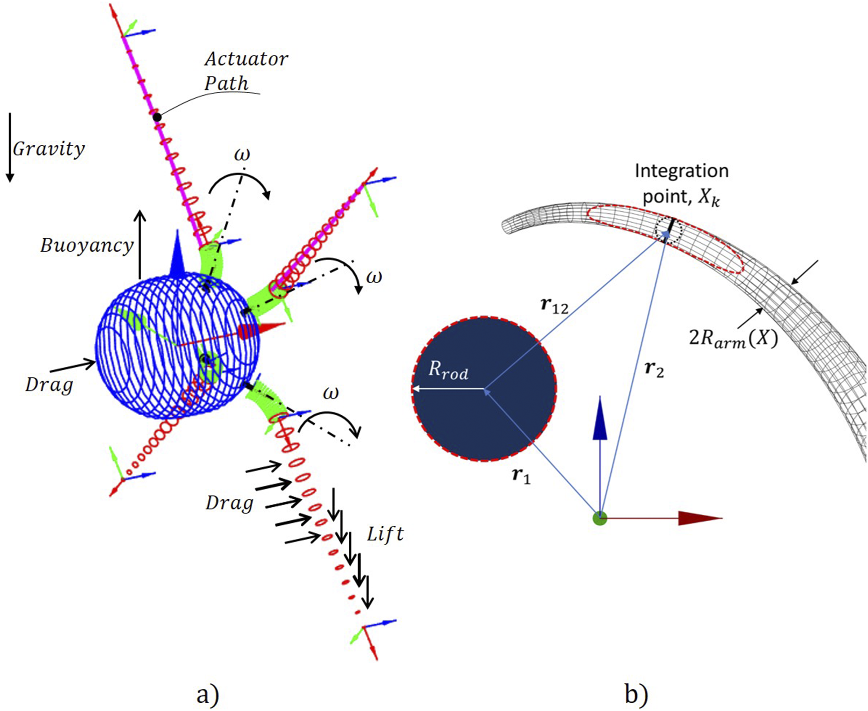
Biological propellers present in prokaryotic bacteria (Rossi et al., 2017) have recently inspired researchers to develop macro-scale underwater propulsion systems. Such propulsion systems, capable of providing noiseless locomotion, were used to develop underwater mobile robots that are deployable in various underwater applications. The appendage, referred to as the flagellum, is imitated by a silicone-based slender body. The flagellum is rotated about a skewed axis with respect to its body axis. The interaction (buoyancy, drag, lift, and water displacement) with water results in an emergent helical shape that produces the propulsion thrust. Experimental validations and dynamic simulations of a four-flagella robot were presented in Armanini et al. (2022a). The authors used a PCS model for the analysis.

We model the mobile robot as an assembly of rigid and soft links as described in Figure 13(a). We simulate a scenario where the robot swims towards a fixed rod and docks itself by gripping onto it, extending our previous work (Mathew et al., 2022b) for two different base choices. The models for fluid interaction are described in Armanini et al. (2022a), while the contact model extends our previous model by introducing a damping factor. Figure 13(b) is a cross-section of the rod and a flagellum at a given y-coordinate. The contact force is defined as

${\mathit{f}}_c=\{\begin{array}{ll}kd+b\dot{d}\frac{{\mathit{r}}_{12}}{\Vert {\mathit{r}}_{12}\Vert }& \text{if}\hspace{0.17em}d>0\hspace{0.17em}\text{and}\hspace{0.17em}\dot{d}>0\\ kd\frac{{\mathit{r}}_{12}}{\Vert {\mathit{r}}_{12}\Vert }& \text{if}\hspace{0.17em}d>0\hspace{0.17em}\text{and}\hspace{0.17em}\dot{d}<0\\ 0& \text{if}\hspace{0.17em}d<0\end{array}$

(46)

where r ₁₂ = r ₂ − r ₁, d = R _arm + R _rod − ‖ r ₁₂‖ and k, b are contact stiffness and damping factors of the model. Note that the contact force model only has a normal component. For the sake of simplicity, we ignore the tangential friction. We also implement a similar contact model between the robot’s shell and the fixed rod.

Figure 13.

(a) Schematic diagram of the mobile underwater robot. The robot’s shell, represented in blue, is modeled as a rigid body with a free joint. Shafts, represented as black cylinders, are rigid bodies with revolute joints. The green hooks are rigid bodies with fixed joints that orient the flagella’s rotation axis. The flagellate arms in red are modeled as inextensible Kirchhoff rods (angular strains only). The top two flagella have thread-like soft actuators, represented by the purple lines. (b) Schematics of the implemented contact model. The red dashed lines represent a cross-sectional cut at a given y-coordinate.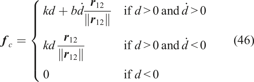

For the dynamic simulation, we use the local FEM linear bases with 3 elements to model the torsional, y-bending, and z-bending strains of each flagellum. This results in a 12-DoF description of the allowed strain fields for each arm. Along with the remaining joints and constraints, the total DoF of the assembly is 58. We rotate the flagella at a constant rate ω = 2π rad/s in pairs in opposite directions to cancel out any resulting moments on the body, preventing unwanted rotation. We rotate the top pair for the first 3 s. Then, for the next 3 s, we rotate the bottom pair. Finally, we rotate all 4 flagella simultaneously for an additional 3 s. Afterward, we allow the robot to slowly approach the rod by stopping the rotation of all flagella for the next 5 s. Figure 14(a) shows the snapshots of the robot locomotion at different times.

Figure 14.

Snapshots of the underwater mobile robot simulation at different times for both (a) Locomotion and (b) Docking scenarios. The dashed red lines represent the trace of the flagellar arm’s tips over the preceding 2 s.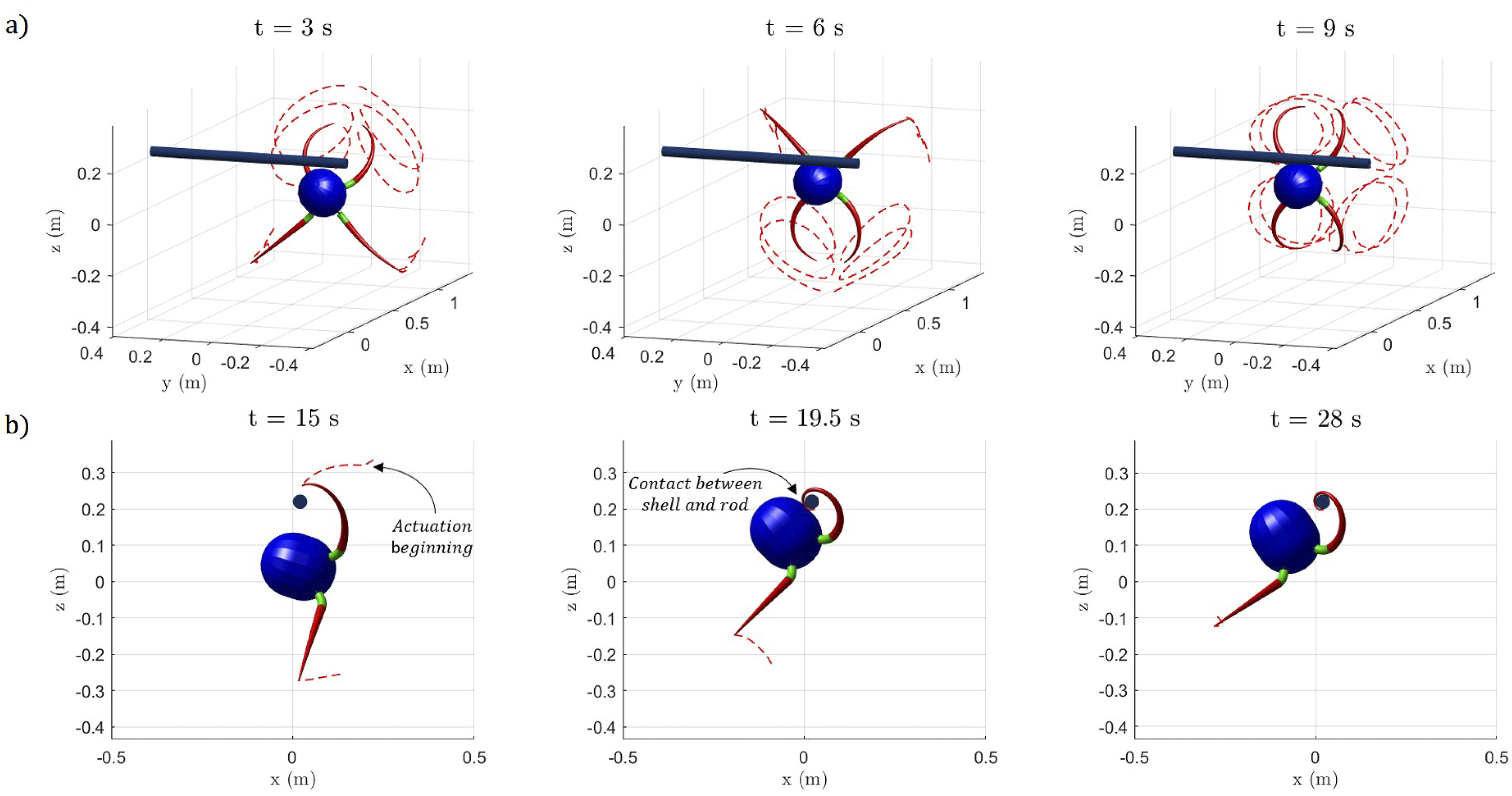

At t = 14 s, once the robot is in close proximity to the docking rod, we linearly ramped the cable tension to 7.5 N in 2.5 s. The distributed actuation force on the flagella together with the contact model enables the grip between the docking rod and the flagella. Due to this, the robot’s shell is pulled towards the docking rod, resulting in a rigid body contact between them at approximately t = 19.5 s. The snapshots of the gripping scenario are presented in Figure 14(b). To compare the performance of the local basis, we redid the simulation using the Legendre polynomials basis with an equivalent DoF (3 ^rd order) for each arm. For the integration of the soft links we used two Gauss quadrature points per element for the local FEM basis, while we used a five-point Gauss quadrature scheme for the global Legendre basis. The local FEM basis simulation took 52.47 min (9.75 min for the locomotion and 42.72 min for the docking phase), while the global basis one took 1 h and 53.05 min (12.68 min for the locomotion and 1 h and 40.37 min for the docking phase) to simulate. The increased computational time for the docking phase is attributable to the abrupt nature of contact events, significantly stiffening the problems and stressing the explicit time-integration scheme employed.

5.3. Wind loading on a suspended cable-driven parallel robot

Recently, 3D printing-based construction has gained attention as a method to print entire buildings or construction components. Due to its low cost and design flexibility, the suspended Cable-Driven Parallel Robot (CDPR) is considered a promising technology for this application (Izard et al., 2017; Tho and Thinh, 2021). Suspended CDPR uses steel wire ropes with high torsional and elongation stiffness relative to their bending stiffness as cables. The inertial and elastic properties of the wire ropes may lead to vibration and sagging, which is difficult to capture using existing models.

To tackle this, we recently developed a model of a four-cable CDPR for the first time using the GVS approach (Mathew et al., 2023) (Figure 15). The CDPR is modeled as a hybrid robot of revolute joints, rigid links (end-effector), and soft links. Three closed-loop joints are introduced to model it as a parallel system. In this work, we study the dynamics of this system when an external force, reminiscent of a wind load, is applied to the end-effector. We approximate the wind load as a periodic unidirectional point force, $f_{EE}\left(t\right)={\left[500\hspace{0.17em}{\sin }^2\left(t\right),500\hspace{0.17em}{\sin }^2\left(t\right),0\right]}^{T}N$ , as shown in Figure 15. To model the bending strains, we used a two-element quadratic FEM basis (5 DoF each). Due to the high torsional and elongation stiffness of the cables, the torsional and elongation strain modes are approximated as constant strains. Hence, the basis is a combination of both global and local bases for the same soft body. This basis definition results in 12 DoF for each cable. Considering the whole assembly with four cables and several rigid joints, the total DoF of the system is 61.

Figure 15.

Schematic diagram of the studied suspended CDPR. Three closed-loop revolute joints (CLJ) are represented by dashed lines. The black circles on the end-effector (EE) represent a 2 DoF universal joint which is elaborated in the inset. The geometric and material parameters of the system are provided in Mathew et al. (2023).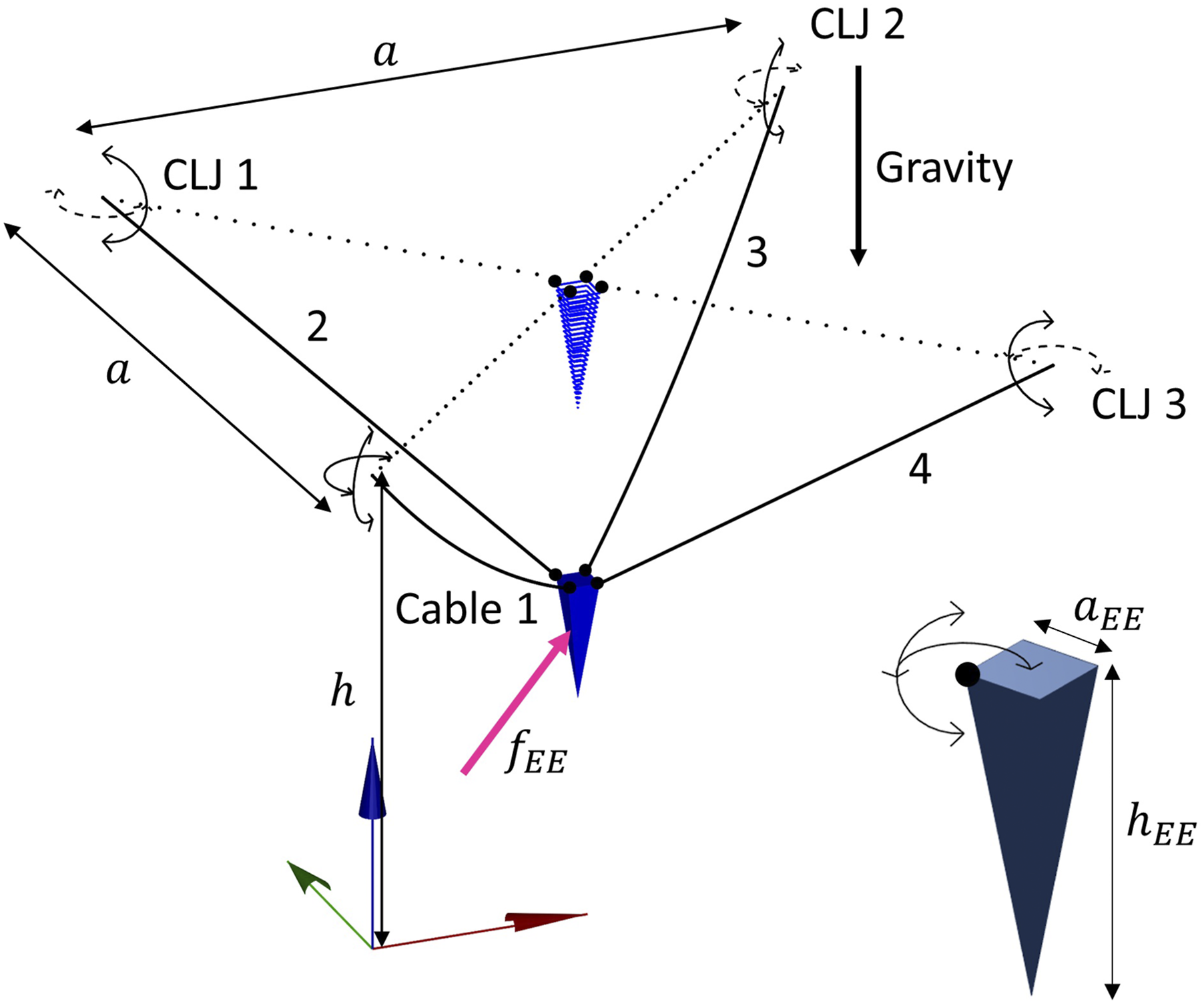

The result of the dynamic simulation is shown in Figure 16. The end-effector tip follows a trajectory in the plane containing the applied load. We can also observe that the cables undergo sagging and exhibit complex vibrations that are captured by the model. The recorded simulation time for 5 s of dynamic analysis of the CDPR was 26.80 min. To compare the simulation speed, we model the bending strains with a global base of equivalent DoF. We used a fourth-order Legendre polynomial basis (5 DoF each) to model the bending strains. The dynamic simulation results were identical, while for the same problem, the simulation took 28.15 min to complete. For the spatial integration of the cables, a five-point Gauss quadrature scheme was used for the global basis, while for the computation using the local basis, we used three Gauss quadrature points per element.

Figure 16.

Snapshots of the four-cable CDPR at different times. An external load is applied end-effector in the form 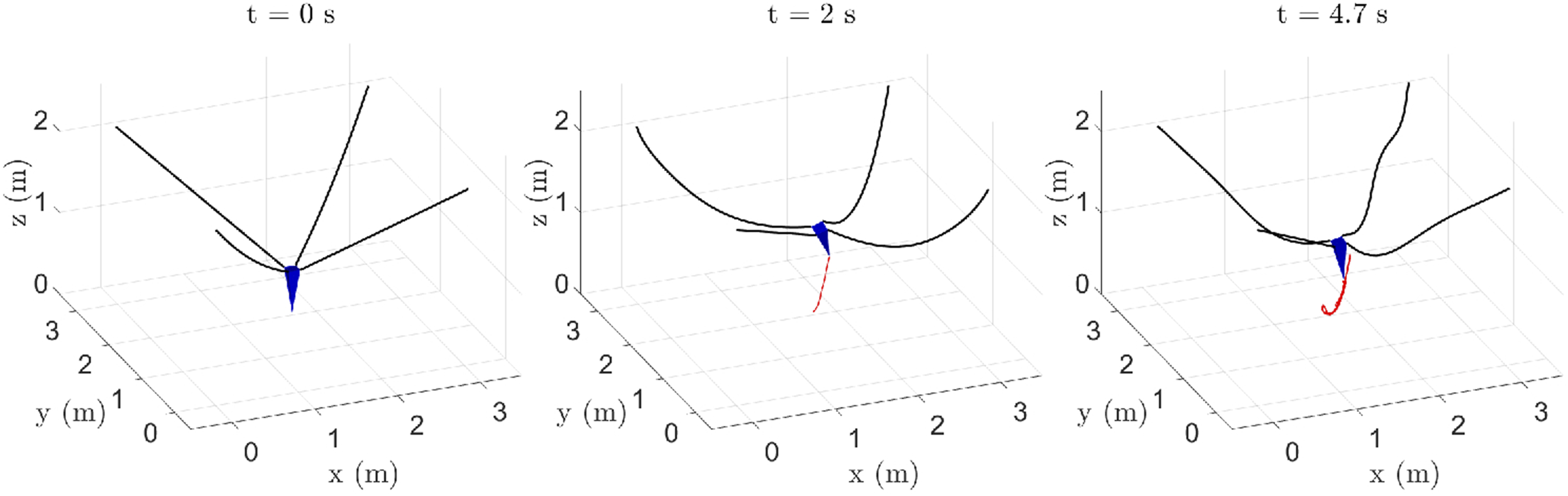$f_{EE}\left(t\right)={\left[500\hspace{0.17em}{\sin }^2\left(t\right),500\hspace{0.17em}{\sin }^2\left(t\right),0\right]}^{T}N$ . For each of the four cables, torsion and elongation strains have a constant basis (1 DoF each), while bending in Y and Z directions are described with a two-element quadratic FEM basis (5 DoF each). The resulting behavior is seen in the trace of the end-effector’s tip (red).

5.4. Dynamics of an octopus arm

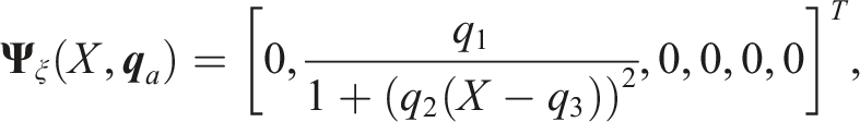
Maneuvers of octopus arms aroused great interest among biologists and engineers a few decades ago. Specifically, the actuation of their arms has recently been studied in different works (Wang et al., 2022; Yekutieli et al., 2005. In Wang et al. (2022), Wang et al. used a non-linear model for the curvature given by κ = kϵ/(1 + (ϵ(s − μ)))². They modeled k as a fixed gain (k = 1.65), μ is the center of the bend, and ϵ is the “extent” of the bend. They compute the actuation moments based on the stiffening wave hypothesis Gutfreund et al. (1998), which alters the stretch and bending stiffness of the arm. The reduced model effectively approximates the bending observed in a real octopus arm. Inspired by this, we study the system dynamics of an octopus arm using a dependent base with our approach.

We model the strain as a combination of the dependent basis function used in Wang et al. (2022) and a second-order monomial basis to capture any additional vibrations of the arm.

$\mathit{\xi }\left(X,\mathit{q}\right)={\mathbf{\Psi }}_{\xi }\left(X,{\mathit{q}}_a\right)+{\mathbf{\Phi }}_{\xi }\left(X\right){\mathit{q}}_b+{\mathit{\xi }}^{*}\left(X\right),$

(47)

where

${\mathbf{\Psi }}_{\xi }\left(X,{\mathit{q}}_a\right)={\left[0,\frac{q_1}{1+{\left(q_2\left(X-q_3\right)\right)}^2},0,0,0,0\right]}^T,$

${\mathbf{\Phi }}_{\xi }=\left[\begin{array}{lll}0& 0& 0\\ 1& X& X^2\\ 0& 0& 0\\ 0& 0& 0\\ 0& 0& 0\\ 0& 0& 0\end{array}\right]$

here $\mathit{q}={\left[{\mathit{q}}_a^T,{\mathit{q}}_b^T\right]}^T$ where, ${\mathit{q}}_a={\left[q_1{q}_2{q}_3\right]}^T$ , and ${\mathit{q}}_b={\left[q_4{q}_5{q}_6\right]}^T$ . q _a corresponds to the generalized coordinates of the dependent basis, while q _b corresponds to that of the independent basis. The dependent part of the strain defers from their model in the following aspects: we do not assume k as a constant, q₁ = kϵ, q₂ = ϵ, and q₃ = μ. The arm is modeled as a conical rod of length l = 0.2 m with a base radius of 1 cm and a tip radius of 0.1 cm, with Young’s modulus of 10 kPa and a density of 1042 kg/m³.

In the simulation, we reproduce the curvature shown in Wang et al. (2022), which is based on recorded data of a real arm octopus. Assuming that the moment has the form ${\mathcal{F}}_i\left(X\right)=\mathbf{\Sigma }\left(\mathit{\xi }-{\mathit{\xi }}_i^{*}\right)$ which matches the static equilibrium solution of strain recorded in Wang et al. (2022). The central point of the bend propagation travels from the half of the arm to the tip in 2 s. This example aims to highlight the strength of our approach to simulate different scenarios and the easiness of combining different bases. To accurately reproduce the physics of the octopus arm, our model also includes external drag, buoyancy, and added mass forces from the displaced fluid (water). Readers may refer to Armanini et al. (2022a) to find the models of fluid interaction. Figure 17 shows the schematics of the problem definition.

Figure 17.

Schematics of the octopus arm. The arm is subjected to internal actuation forces and external loads.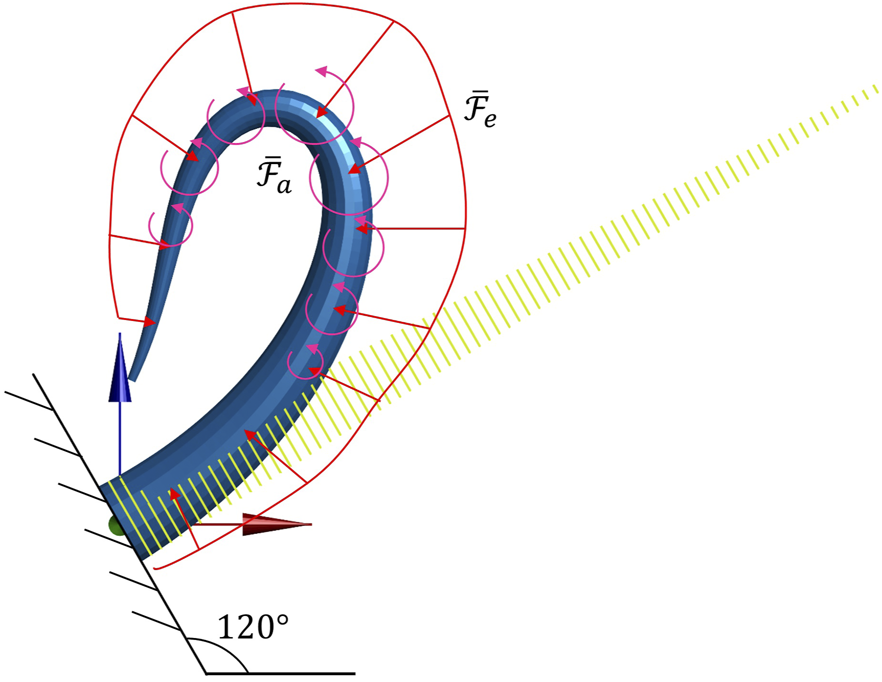

Snapshots of the arm shape and their corresponding strain profile are shown in Figure 18. It is observed that the results appear realistic and allow us to represent the bending propagation of an octopus arm. Also, it is important to highlight that our approach is able to capture the vibration of the system. The vibration is more noticeable in the part of the arm close to the tip because the cross-section is smaller (see the three first snapshots of the strain where the value of the strain close to X = 1 varies from zero to a negative value and after to a positive value in a very short period of time). Moreover, the proposed bases (6 DoF) is compared with FEM Cubic 10 elements (31 DoF). The figure illustrates a very high similarity between the two cases. Notably, the dependent bases exhibit significantly fewer degrees of freedom, suggesting the potential utility of dependent bases in certain scenarios. The simulation time for the dependent bases was 18.91 s, while the FEM case took 174.72 s to complete, both using the ode45 integrator of MATLAB.

Figure 18.

Snapshots of the octopus arm simulation using the proposed dependent bases. The shape of the arm and the strain through the tentacle is represented in the upper and lower part of the figure, respectively. The Snapshots depict the simulation where the bend propagation of the octopus arm travels from the half of the arm to the tip in 2 s. In the simulation, only bending in Y using the combined dependent basis (47) is used to describe the bending propagation of the octopus arm. The proposed bases (black line) is compared with FEM Cubic 10 elements (blue line). The red rectangles point out the effect of adding a second-order monomial basis to capture the vibration of the octopus arm.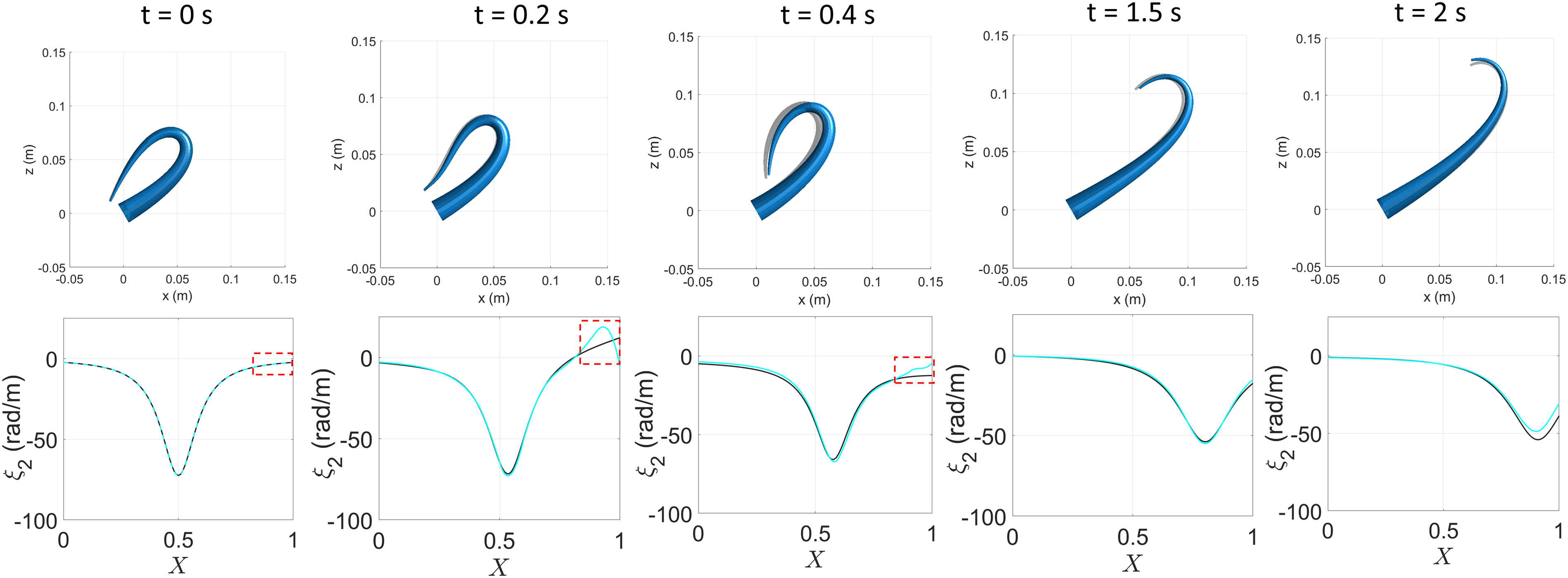

6. Discussions and conclusions

In this paper, we presented the complete formulation of the GVS model. We described a recursive computation of forward kinematics, velocities, and accelerations. With this, we emphasized that the GVS approach models the rigid joints and soft links under the same framework. We introduced “dependent” strain bases, the most general form of strain parameterization, where the strain basis is a non-linear function of generalized coordinates and time. Independent strain bases (not functions of q and t) are a subset of dependent bases. To project the free dynamics of the system into the space of generalized coordinates, we derived a recursive Geometric Jacobian formula for both cases. Our current implementation computes the kinematic variables like the Jacobian at every temporal instance and computational point, ensuring maximal precision for the computation of the system’s dynamics. However, in scenarios where the numerical derivative of the Jacobian evolves slowly or when the robot undergoes small deformations, the Jacobian may not need to be computed at every time instance and at every computational point in order to accelerate the computational process. Considering the trade-offs between accuracy and computational speed, future implementations of the model could investigate the use of reduced resolutions to enhance computational speed.

We compute the components of the generalized dynamics and statics equations using a two-level nested quadrature scheme. The equivalence of rigid joints and soft links, recursive computation of kinematics and their derivatives, and the nested quadrature integration scheme call for a simple algorithm for dynamic and static analyses. The paper includes a three-part Appendix that runs in tandem with the presented model, serving as a guide for readers to develop their own program for specific robotic applications using the GVS model.

Based on the domain of the basis functions, independent bases are further classified into global and local bases. We discussed a few examples of global bases and generalized the concept of FEM-like local bases. For FEM-like bases, the value of the generalized coordinates corresponds to the value of the strain at the element nodes. This makes the modeling relative nodal reduction. The value of the generalized coordinates of FEM-like bases is intuitive and may prove advantageous for the state estimation of the system. We demonstrated the accuracy of the local basis over the global basis by comparing a simulation result with that obtained from a commercial FEM package. To study the relative speed of simulation for global and local bases, let us consider the first three applications of Section 5. Table 4 compares the simulation speed when using global or local bases. The variable t _r represents the ratio between the computational time and the real-time duration for which the computation is performed.

Table 4.

Computational speed and position mismatch of different bases solutions for the applications in Section 5.

App	Basis type	DoF	Integrator	t r	Avg. Mismatch (%)
5.1	Legendre	30	ode15s	1.85	2.06
	FEM quadratic			2.28
5.2	Legendre	58	ode15s	226.10	0.86
	FEM linear			104.93
5.3	Legendre	61	ode113	337.80	0.64
	FEM quadratic a			321.60
5.4	Dependent	6	ode45	9.45	3.39
	FEM cubic	31		87.36

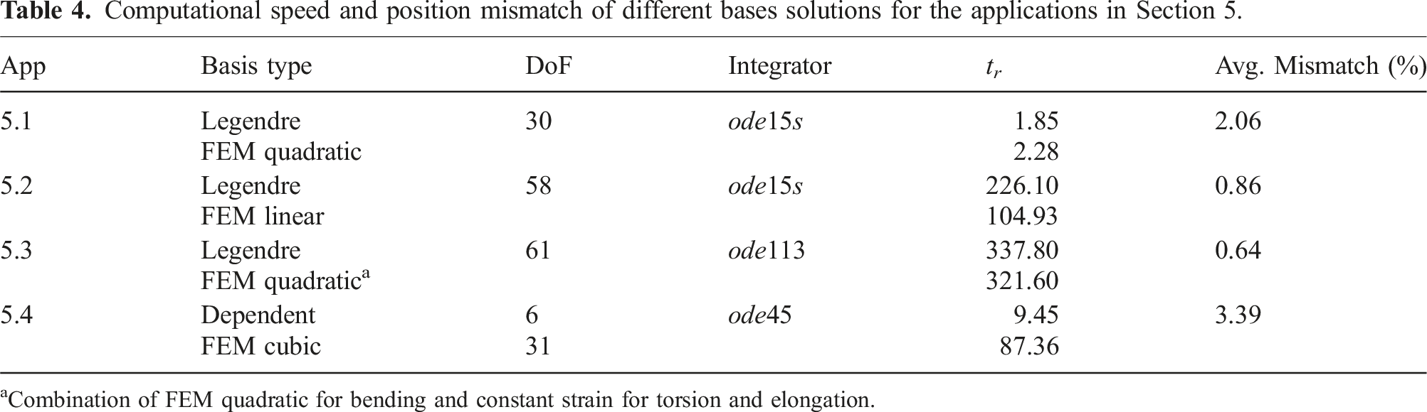
^aCombination of FEM quadratic for bending and constant strain for torsion and elongation.

The first three applications presented in Section 5 compare global and local independent bases. In comparing models, we utilized an equal number of DoFs to maintain a consistent baseline for assessing the computational speed. It was observed that, within the specific cases studied, global and local bases with the same DoFs captured similar body position as shown in Figure 19, with minimal mismatch (quantified at less than a 5% difference as reported in Table 4). As for the fourth application, the dynamics of the dependent basis case presented in Section 5.4 using 6 DoFs is compared with that of a 10 element, cubic FEM basis of 31 DoFs. The mismatch is quantified with a maximum of 6.59% and an average of 3.39%, even though one fifth of the DoFs of the local basis case were used for the dependent basis case. The global Legendre basis performs better (23% faster) for the analysis of cable-driven soft manipulators (Section 5.1). In this case, the external force (gravity) and internal actuation loads are of a distributed nature. Global bases, where the basis function spans the entire length, are ideal for capturing such cases. The second example of locomotion and docking of the underwater robot (Section 5.2) is where the true potential of the local basis is revealed. Due to the local contact events and boundary loads, the local FEM basis performs exceptionally better (215% faster) in this case. In the third application of suspended CDPR (Section 5.3), the steel wire ropes are subjected to significant boundary loads. The two different bases considered for this application are: (1) a hybrid global-local basis, which employs a FEM-like basis for bending strains and a global constant strain basis for torsion and elongation, and (2) a Legendre polynomial basis with the same DoFs The hybrid basis performs marginally better in this case: 5% faster. This example also highlights the ability of the model to combine both global and local bases. There are a few limitations for FEM-like bases that warrant consideration: (i) To model different orders of strain for multiple modes of strain, a different number of elements for each strain mode may be needed, increasing the computational cost. (ii) As noted earlier, the minimum DoF for linear, quadratic, or cubic basis is 2, 3, and 4, respectively. (iii) The strain distribution is prone to C1 discontinuity at element boundaries.

Figure 19.

Comparative analysis of different bases solution for the applications discussed in Section 5. (a) Tip trajectory from the solutions of global and local bases for the cable-driven manipulator (Section 5.1). The mismatch between them, normalized by the manipulator’s length (30 cm), is shown as inset. (b) The trajectory of the shell’s center of the underwater soft robot (Section 5.2) from global and local bases solutions. The mismatch between them, normalized by the shell length (20 cm), is shown as inset. (c) The end-effector tip trajectory of global and hybrid bases solutions for the cable-driven parallel robot (Section 5.3). The mismatch shown in the inset is normalized using cable length (2.47 m). d) Tip trajectory of the Octopus Arm (Section 5.4) of the dependent and local bases solutions. The mismatch between both tip trajectories, normalized by the arm length (20 cm), is shown as inset. The circles indicate the beginning of the simulations (t = 0), while the squares indicate the end.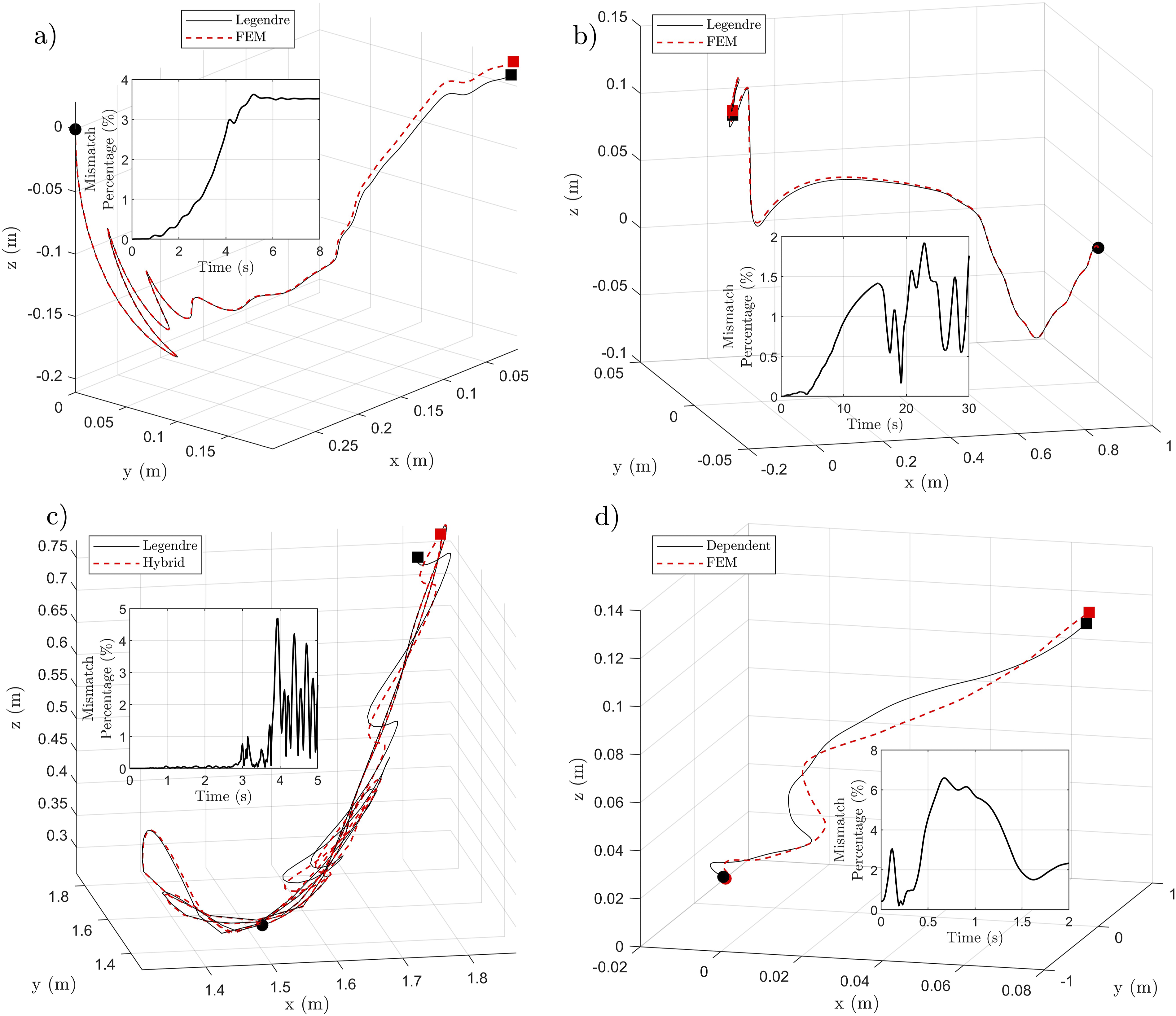

Dependent bases open a new spectrum of bases tuned for order reduction for specific problems. They are ideal for cases when we expect the strain to follow a specific shape. This is emphasized by the illustrative examples in Section 4. Figures 9 and 10 highlight that the dependent basis effectively models the strain profile with very few DoF compared to independent bases. In dynamic simulations, where the system vibration is relevant, combining dependent bases with independent bases is ideal, as demonstrated in Section 5.4. While combining different bases, one must ensure they are not linearly dependent. Consider this case where the bending strain, ${\mathit{\xi }}_2=q_1+q_2{e}^{q_{3}X}$ . When q₃ is zero, the generalized coordinates q₁ and q₂ are redundant (linearly dependent). This may lead to numerical instabilities during dynamic simulations. While dependent bases perform well in specific problems, in general, if the deformed shape of the Cosserat rod is unpredictable, it is better to use a global or local independent basis.

The SoRoSim toolbox was introduced to provide a GUI-based black-box experience for users from different backgrounds. We updated the toolbox with all the basis functions presented in this work. We used the new version of the SoRoSim toolbox to perform all simulations presented in this paper. A generic pseudo-code for creating and simulating a robot in SoRoSim is provided in Appendix D. In addition to static and dynamic simulations, the toolbox can be combined with custom-made codes or MATLAB packages to optimize, control, or estimate robotic systems. The new version of the toolbox is available at MATHWORKS and GitHub (Ben Hmida and Mathew, 2023). The executable scripts for the four examples mentioned in Section 5 are available via the GitHub link. New users can find introductory tutorials (MATLAB live scripts) and examples within the SoRoSim source code. The SoRoSim user manual file, along with the YouTube links provided on the website, can assist new users in utilizing SoRoSim. We hope to see the Geometric Variable Strain approach being implemented and the SoRoSim toolbox being used in separate studies.

Supplemental Material