
Abstract
Algorithms that use derivatives of governing equations have accelerated rigid robot simulations and improved their accuracy, enabling the modeling of complex, real-world capabilities. However, extending these methods to soft and hybrid soft-rigid robots is significantly more challenging due to the complexities in modeling continuous deformations inherent in soft bodies. A considerable number of soft robots and the deformable links of hybrid robots can be effectively modeled as slender rods. The Geometric Variable Strain (GVS) model, which employs the screw theory and the strain-parameterization of the Cosserat rod, extends the rod theory to model hybrid soft-rigid robots within the same mathematical framework. Using the Recursive Newton-Euler Algorithm, we developed the analytical derivatives of the governing equations of the GVS model. These derivatives facilitate the implicit integration of dynamics and provide the analytical Jacobian of the statics residue, ensuring fast and accurate computations. We applied these derivatives to the mechanical simulations of six common robotic systems: a soft cable-driven manipulator, a hybrid serial robot, a fin-ray finger, a hybrid parallel robot, a contact scenario, and an underwater hybrid mobile robot. Simulation results demonstrate substantial improvements in computational efficiency, with speed-ups of up to three orders of magnitude (1000x). We validate the model by comparing simulations done with and without analytical derivatives. Beyond static and dynamic simulations, the techniques discussed in this paper hold the potential to revolutionize the analysis, control, and optimization of hybrid robotic systems for real-world applications.
1. Introduction
Rigid-body algorithms have been developed for the mechanical analysis of multi-body systems, enabling the modeling of dynamic response and static equilibrium of robots (Featherstone, 2008; Murray et al., 1994). Over the years, these algorithms have undergone remarkable improvements, enabling faster-than-real-time simulations (Newbury et al., 2024). One of the most significant advancements has been the incorporation of gradient information into these algorithms (Carpentier et al., 2019; Howell et al., 2023; Giftthaler et al., 2017a; Geilinger et al., 2020). The ability to accurately and efficiently compute the derivatives of governing equations with respect to the system’s state, model parameters, and control variables has been pivotal for implicit integration, design optimization, trajectory optimization, and optimal control. The impact of these advancements is exemplified by leading humanoid and quadrupedal robots, such as those developed by Boston Dynamics and Unitree (Bjelonic et al., 2022). These robots leverage the gradient information for trajectory optimization and model-predictive control (MPC), enabling real-time control, enhanced stability, and adaptability in complex environments (Sukhija et al., 2023; Neunert et al., 2018; Wensing et al., 2024).
Several methods exist for computing the derivatives of governing equations, each with its trade-offs (Newbury et al., 2024). The most straightforward approach is the numerical scheme of finite difference. The finite difference method can offer simplicity and ease of parallelization but often falls short in accuracy (Todorov et al., 2012). Automatic differentiation (AutoDiff) computes derivatives by recognizing that even complex functions are built from fundamental operations and functions. It systematically applies the chain rule to these operations within the algorithm, allowing the program to automatically calculate derivatives alongside the original calculations (Tedrake and the Drake Development Team, 2019; Giftthaler et al., 2017b). However, AutoDiff involves intermediate computations that are generally hard to simplify. Analytical methods take a manual approach by directly applying the chain rule to recursive algorithms like the Recursive Newton-Euler Algorithm (RNEA) (Carpentier and Mansard, 2018; Singh et al., 2022). By exploiting the inherent structure and spatial algebra at the core of rigid-body dynamics algorithms, analytical derivatives (AD) can simplify computations and achieve greater computational efficiency than automatic differentiation methods. Efficient implementation of analytical derivatives can lead to faster and more resource-efficient computations with improved accuracy and provide deeper insight into the mathematical structure of the derivatives. However, deriving analytical derivatives manually can be complex and time-consuming, making them challenging to implement (Singh et al., 2022).
Deriving analytical derivatives in soft robots is significantly more challenging than in rigid-body systems. The primary difficulty stems from the complex nature of deformable bodies, which undergo large, continuous deformations, making it highly challenging to derive closed-form equations for their dynamics. The general class of soft robots, which cannot be modeled as a system rods, require numerical methods based on 3D continuum mechanics such as Finite Element Methods (FEM) (Duriez, 2013) or Material Point Method (MPM) (Hu et al., 2018). Analytical derivatives of FEM in robotics have been explored in several works, including Hoshyari et al. (2019); Hafner et al. (2019); Geilinger et al. (2020); Bächer et al. (2021); Jatavallabhula et al. (2021); Du et al. (2022). On the other hand, MPM is often referred to as naturally differentiable due to its particle-grid representation and the smooth interpolation between particles and the grid, which makes gradient computation more efficient (Spielberg et al.. 2023; Huang et al., 2021). FEM and MPM use maximal coordinate representations for rigid bodies, increasing the degrees of freedom (DoF) and the computational cost for hybrid soft-rigid robots.
A large portion of soft robots and the compliant links of hybrid soft-rigid robots can be effectively modeled as slender, rod-like structures, making them well-suited for analysis using the Cosserat rod theory (Armanini et al., 2023). The Cosserat rod is a 1D continuum mechanics object that can model deformations of slender bodies, including twisting, bending in two axes, stretching, and shearing in two axes (Cao and Tucker, 2008). Four distinct research communities have leveraged Cosserat rod theory to address their specific challenges, each producing specialized numerical methods tailored to their needs. Ranking them by their order of appearance, these communities are: the geometrically exact FEM community, the ocean engineering community, the computer graphics community, and the robotics community. The geometrically exact FEM community has focused primarily on developing FEM software that can predict the movements and stresses of mechanisms undergoing large deformations (Simo and Vu-Quoc, 1988; Meier et al., 2017; Eugster and Harsch, 2023). Meanwhile, the ocean engineering community has applied Cosserat rod models to the simulation of towed submarine cables, addressing the unique challenges posed by underwater environments (Burgess, 1992; Tjavaras et al., 1998). On the other hand, the computer graphics community has prioritized computational speed for interactive simulations of filament-like structures, such as hair, using the Discrete Elastic Rod (DER) approaches (Bergou et al., 2008; Gazzola et al., 2018). Finally, the robotics community has concentrated on the simulation and control of soft or continuum robots to safely interact with their surroundings (Rucker and Webster, 2011; Till et al., 2019; Boyer et al., 2022).
To cater specifically to the needs of robotics, a novel parameterization of the configuration space of Cosserat rods has been proposed, focusing on strain fields rather than the traditional pose-based approach used in FEM and DER. This strain-based approach, referred to as the Geometric Variable Strain (GVS) method (Renda et al., 2020; Boyer et al., 2020), is geometrically exact and aligns well with the demands of soft robotic applications. The GVS approach provides a reduced-order formulation with the least number of generalized coordinates for modeling their dynamic and compliant behavior. Among the various models based on the Cosserat rod, the GVS model stands out for its ability to merge the screw theory-based formulation of rigid robots with the strain-parameterization of the rod. Its Lagrangian mechanics formulation with minimal generalized coordinates enables efficient analysis of hybrid soft-rigid robotic systems within a unified mathematical framework (Figure 1). The implementation of the GVS model, based on the approximate Magnus expansion of the rod’s strain field, makes the soft body computationally equivalent to multidimensional, discrete rigid joints (Mathew et al., 2024). Hence, the strain-parameterization of our formulation aligns more closely with traditional rigid-body models than alternative methods, ensuring compatibility with established robotics frameworks. The model has been extensively validated through comparisons with analytical models, FEM, and other rod models (Boyer et al., 2023; Mathew et al., 2022a; Tummers et al., 2023), as well as experimental studies (Alkayas et al., 2025; Feliu-Talegon et al., 2024; Tummers et al., 2024). In Mathew et al. (2022a, 2024), we implemented the GVS model for hybrid soft robots using a built-in implicit integration scheme in MATLAB called ode15s. When analytical derivatives (Jacobian) are not supplied, ode15s internally compute the Jacobian of the governing equations using a finite difference scheme. However, this can lead to longer computational times or cause the solver to stall due to errors introduced by the numerical approximation, particularly in high-DoF systems with constraints. The objective of this work is to develop and implement an analytical derivative for the GVS model, aiming to improve computational efficiency and robustness in the simulation of hybrid soft-rigid robots. In the GVS model, a rigid joint is equivalent to a fictitious constant strain Cosserat rod and a soft body is equivalent to an infinite series of rigid joints. The infinitesimal change in configuration is captured by the local velocity 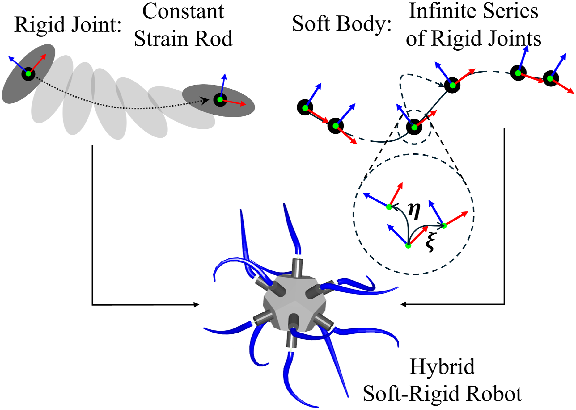
Related works: The Piecewise Constant Strain (PCS) model, which discretizes the continuous deformation of a Cosserat rod into a finite number of segments with constant strain, is a subclass of the GVS model. Based on the Comprehensive Motion Transformation Matrix (a Lie group of coordinate transformations of displacement, velocity, and acceleration), an analytical gradient of the PCS model was derived in Ishigaki et al. (2024). A differentiable soft robot simulation environment called DisMech was introduced based on the implicit DER method (Choi et al., 2024). DisMech employs a finite difference scheme to compute the necessary gradients for the implicit integration. Recently, a new algorithm for the implicit dynamics of robots with rigid bodies and Cosserat rods has been proposed (Boyer et al., 2023). By applying an exact symbolic differentiation of the robot’s RNEA inverse dynamics (named IDM in Boyer et al. (2023)), a new RNEAlgorithm, called the tangent inverse dynamics model (TIDM), has been derived. This algorithm is then fed with unit inputs to numerically calculate the Jacobian of the inverse dynamics. This calculation is performed at the continuous level, that is, directly on the partial differential equations (PDEs), and before spatial integration, for which spectral methods have been employed instead of Magnus expansion. Although the approach adheres to the true definition of geometrically exact methods—where discretization of time and space occurs only after all analytical calculations—due to its implicit nature, it does not directly provide Jacobian matrices in analytical matrix form, which can be advantageous for control and fast simulation of robots with MATLAB. In contrast, the approach here presented lies in its analytic and explicit formulation, which was made possible by the Magnus expansion.
Contributions of this work: By leveraging the “pseudo-rigid joint” formulation of GVS and building upon established methods for analytical derivatives in rigid-body systems (Carpentier and Mansard, 2018; Singh et al., 2022), we developed analytical derivatives for soft and hybrid soft-rigid robots with slender soft bodies. While Mathew et al. (2024) formulated the governing equations of the GVS model for a hybrid soft-rigid robot, focusing on various strain-parameterizations and the computational procedure, this paper focuses on deriving their analytical gradients and developing an efficient algorithm for their computation. We implemented the derivatives in two implicit integration algorithms: ode15s of MATLAB and Newmark-β scheme for dynamics and provided the analytical Jacobian for efficient static equilibrium computation. Our method significantly improved the computational speed of implicit integration for dynamic simulations, achieving speed-ups of up to three orders of magnitude compared to traditional methods without analytical derivatives. Similarly, for static analysis, we observed substantial improvements in computational efficiency. Six common robotic systems are considered for the simulation study. Additionally, we implemented the theory developed in this paper into our GUI-based MATLAB toolbox, SoRoSim, making it a fully differentiable robotics toolbox capable of modeling generic hybrid soft-rigid robots with slender soft rods. (Mathew et al., 2025b). To the best of the authors’ knowledge, this is the first work to derive and implement analytical derivatives for the mechanical analysis of hybrid soft-rigid robotic systems of this kind.
(1) Derivation of the analytical gradient of the GVS model. (2) Integration of the gradient information for static and dynamic simulations. (3) Analysis of different robotic systems validating the analytical gradient and demonstrating computational efficiency. (4) Integration of the theory into the SoRoSim toolbox, making it a differentiable tool for modeling hybrid soft-rigid robots.
Organization of the paper: A summary of the GVS model is presented in Section 2. Section 3 details the implementation of analytical derivatives in dynamic and static algorithms for fast and accurate computations. In Section 4, we focus initially on a single soft body, applying the RNEA and ID framework to derive the analytical derivatives of the governing equations. This framework is extended to hybrid multi-body systems in Section 5. We address two typical constraints in multi-body systems: joint actuation via joint coordinates and closed-chain (CC) systems. Section 6 discusses the derivation of analytical derivatives for systems subjected to three common external forces: point forces, contact loads, and hydrodynamic forces. Simulations and validations across six robotic systems are presented across these sections, demonstrating the effectiveness of the approach.
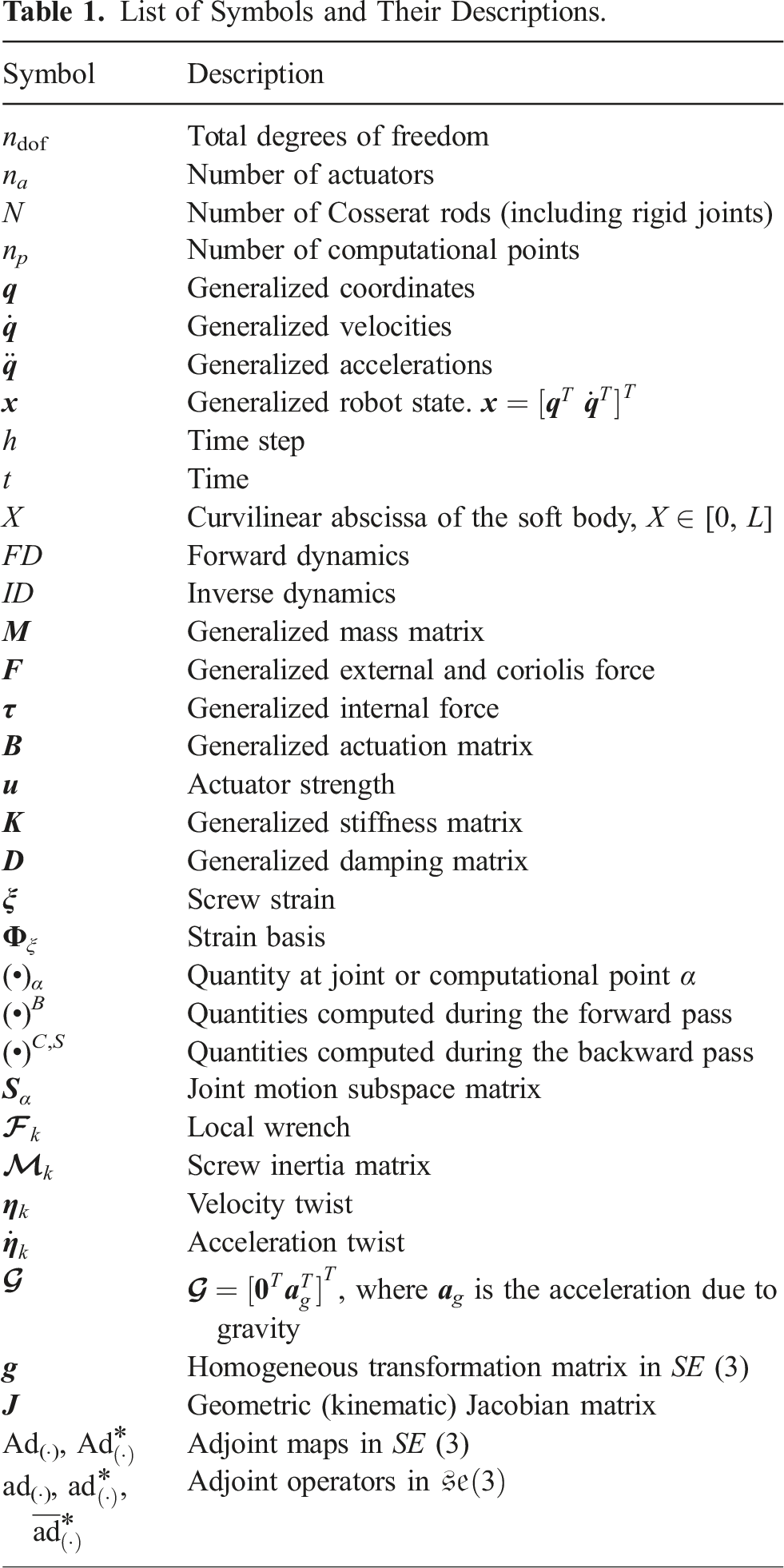
List of Symbols and Their Descriptions.
2. Summary of the GVS model
The GVS model introduces generalized coordinates (
For a hybrid robot with N Cosserat rods (including rigid joints and soft bodies), the state of the robot
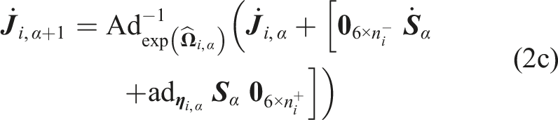
Using these, a recursive scheme that employs the exponential map of the Lie algebra of SE (3) is implemented to compute the robot’s forward and differential kinematics (Appendix A). This yields 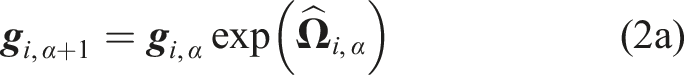

where,
Based on D’Alembert’s principle, the free dynamics of soft links and rigid bodies are projected onto the generalized coordinate space using the geometric Jacobian (Kane method (Kane and Levinson, 1983)), yielding the generalized mass matrix 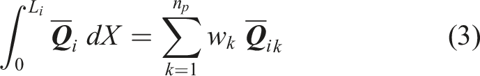
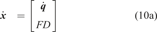
Finally, the Forward Dynamics (FD) computes 
Figure 2 presents a graphical summary of the model implementation. The dynamic simulation computes the temporal evolution of the robot’s state by time-integrating Graphical summary of the GVS model: (a) Schematic of the implemented recursive scheme and (b) block diagram showing the summary of the GVS FD algorithm.
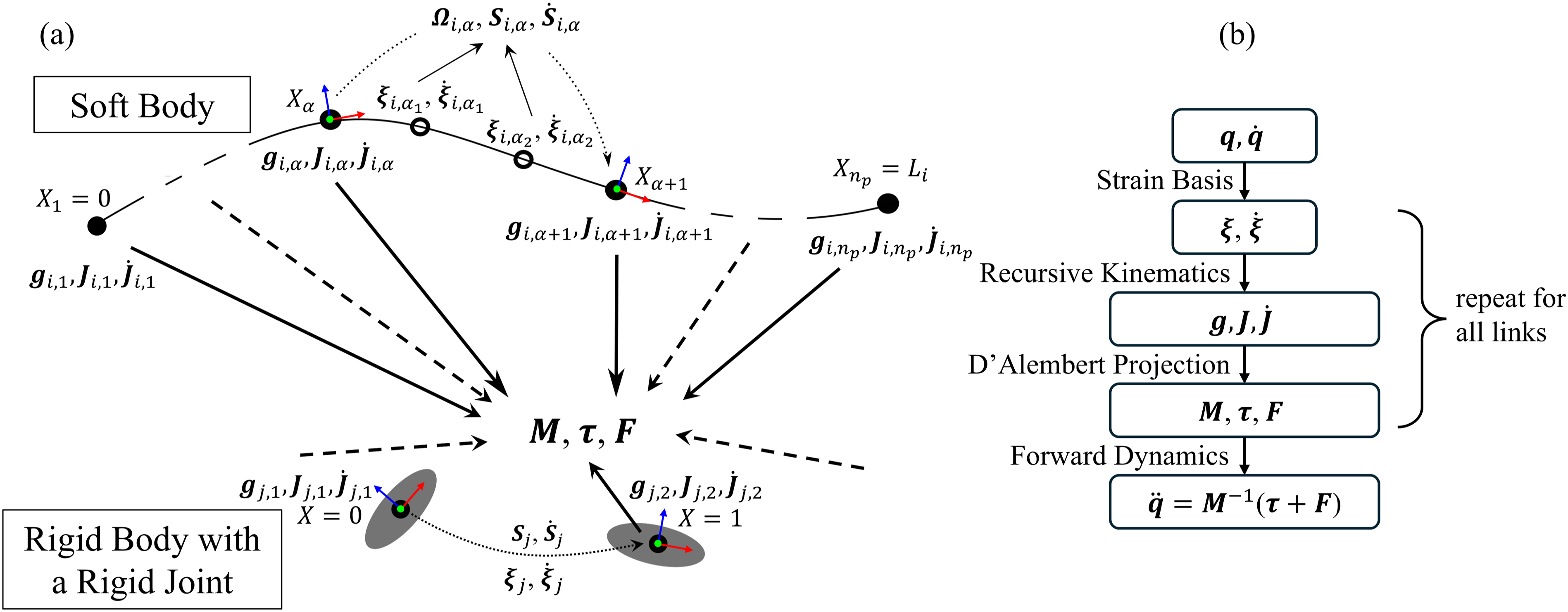
For further details on the model and its computational implementation, readers are encouraged to refer to Mathew et al. (2024).
3. Derivatives for dynamics and statics
Analytical derivatives of governing equations, (4) and (5), are crucial for efficiently solving dynamic and static problems. Here, we explain how the derivatives can be utilized to ensure accurate and fast computations.
3.1. Implicit Euler integration using inverse dynamics
The temporal evolution of the robot state
The explicit Euler method is given by
For an explicit integrator, 
Since 
The Jacobian of this equation is given by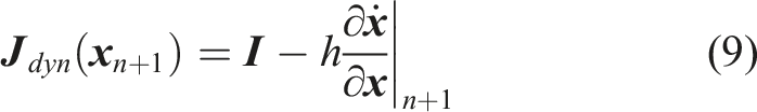
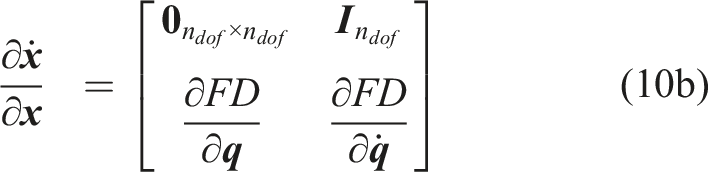
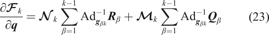
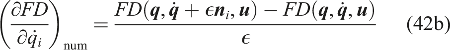
While the Jacobian can be computed numerically or analytically, the analytical computation can provide faster and more accurate results. To obtain the derivatives of FD for the computation of the Jacobian, we take a partial derivative of equation (4) with respect to 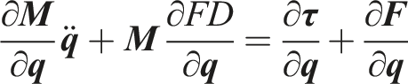
By rearranging terms, we get: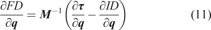

Similarly, we get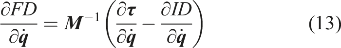
3.2. Newmark-β method
The Newmark β method is another advanced implicit scheme, widely used in structural mechanics where it has been improved over the years thanks to the HHT or the Generalized-α-method among others (Cardona and Géradin, 1994; Chung and Hulbert, 1993). Recently, it has been shown that the Newmark scheme is symplectic and variational (Kane et al., 2000), which may explain the reasons for its success in the FEM community. In the Newmark scheme, 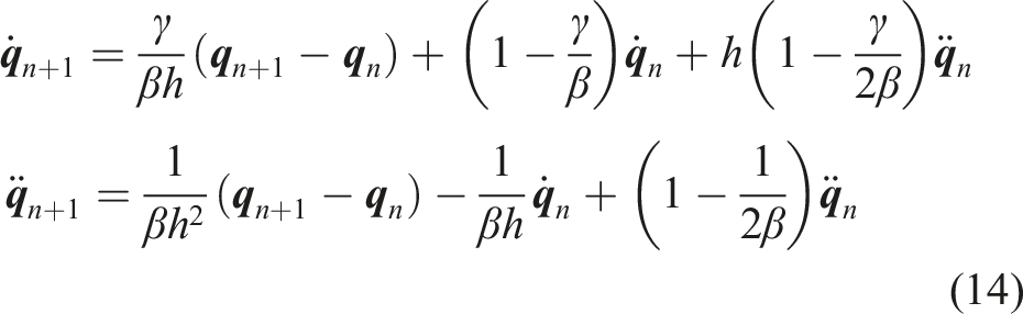

The solution for
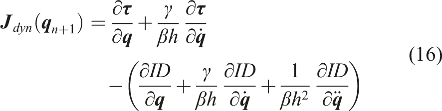
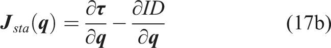
3.3. Computation of static equilibrium
The role of the Jacobian in the statics simulation is straightforward. The residual and Jacobian for solving the static equilibrium can be derived from equations (5) and (12) with 
Numerical solvers such as fsolve in MATLAB, use (17a) with an initial guess
4. Derivatives of soft body dynamics
We begin by deriving the derivative for a single soft body and then extend this approach to a hybrid multi-body system. For simplicity, we omit the subscript i in this section. By virtue of the Magnus expansion, the soft body is computationally equivalent to n
p
− 1 rigid joints governed by the same Schematic of the RNEA for a single soft body showing the forward pass for kinematics and the backward pass for joint wrench computation. The joint motion subspace (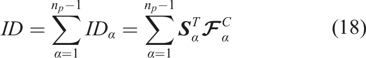

With this we proceed to compute the partial derivative of ID with respect to the states of the robot. A summary of the results is presented below. For detailed derivations, readers are encouraged to refer to Appendixes C and D.
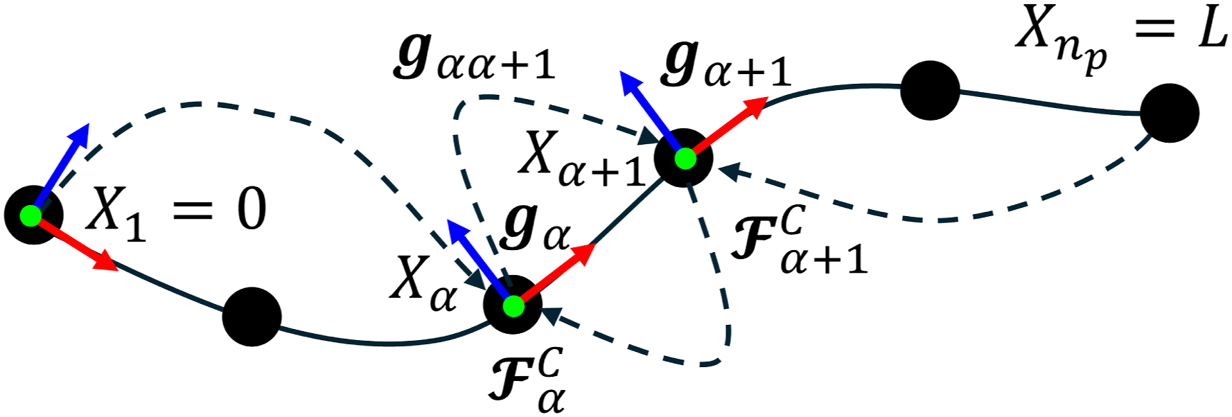
4.1. Partial derivative of ID with respect to generalized coordinates
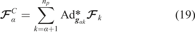
Substituting equations (19) in (18), we can see that the partial derivative of ID
α
with respect to 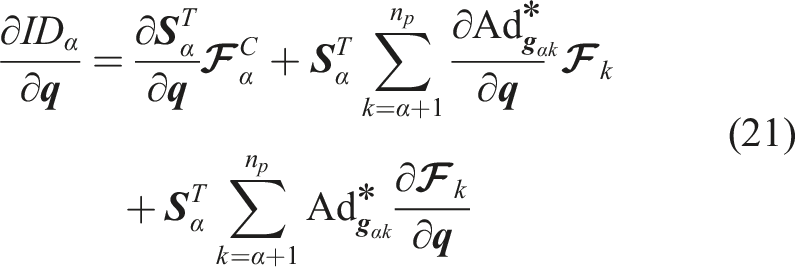
The analytical formula for the first term is provided in the Appendix C. The second and third terms involve sum over k from α + 1 to n
p
. The derivations of their summands are given in the Appendix D. We get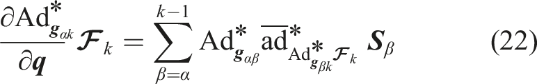

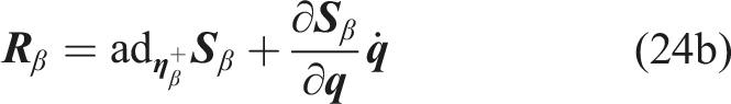

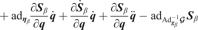
The definitions of the adjoint operators and the analytical formulas of 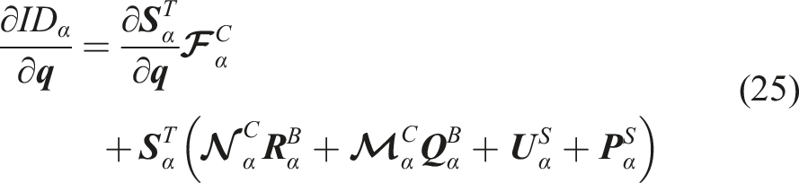


Finally, we obtain: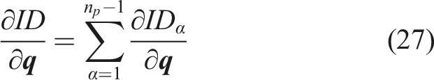
Note that
4.2. Partial derivative of ID with respect to generalized velocities
The partial derivative of ID
α
wrt 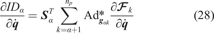
Only the Coriolis force is a function of 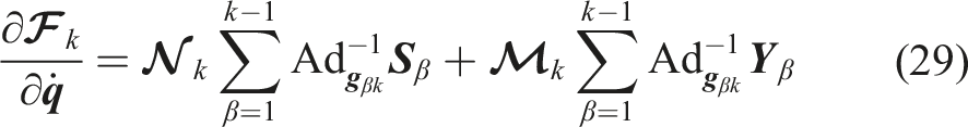

Substituting equations (29) into (28) and taking the sum over k from α + 1 to n
p
, we get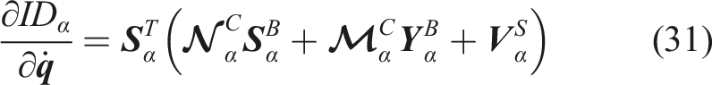


Note that
Summing equation (31) over α from 1 to n
p
− 1, we have: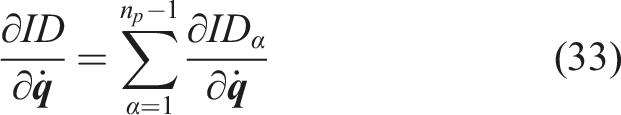
4.3. Partial derivative of ID with respect to generalized accelerations
The partial derivative of ID
α
with respect to 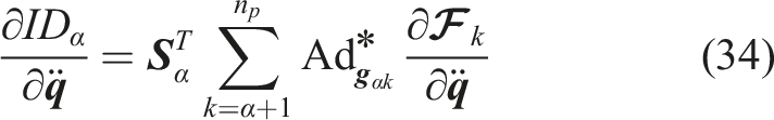
Only the inertial force is a function of 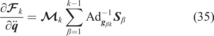
Substituting this into equation (34), we get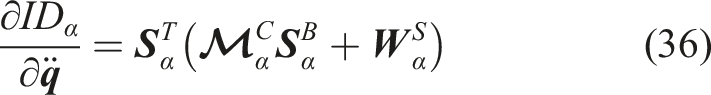

Finally summing over all α, we get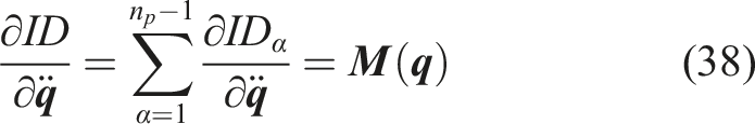
Note that equation (38), incidentally, represents a novel way of computing the generalized mass matrix of a soft robot.
4.4. Partial derivatives of internal forces
The internal forces include the elastic, damping, and actuation forces. It is given by
The actuation matrix (
The partial derivative of 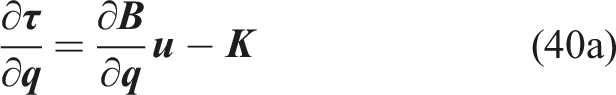
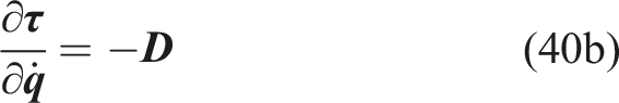
For tendon-like actuators, the partial derivative of
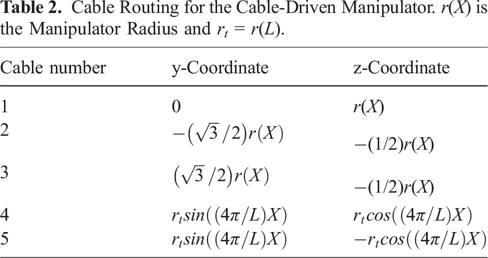
4.5. Cable-driven soft manipulator
Based on the results so far, we set up the first simulation example. We simulate a cable-driven soft manipulator (CDM) shown in Figure 4(a). The manipulator radius varies linearly from base to tip according to r(X) = r
b
+ (r
t
− r
b
)X/L. The material properties used in the simulation are as follows: Young’s modulus of 1 MPa, Poisson’s ratio of 0.5, density of 1000 kg/m3, and a material damping coefficient of 104 Pa ⋅s. The soft manipulator has five tendon-like actuators, as shown in Figure 4(a). Their routing, local coordinates for a given X, are provided in Table 2. Gravity acts in the negative z-axis direction. We used a Legendre polynomial basis with 4th-order angular strains (torsion about x, bending about y and z) and 2nd-order linear strains (elongation about x, shear in y and z). Hence, the total DoF of the system is 24. For the numerical integration, we used 5 Gauss quadrature points. Including the computational points at the base and the tip, the total number of points n
p
= 7. (a) Schematics of cable-driven soft manipulator with cable routing. L = 50 cm, base radius r
b
= 3 cm, and tip radius r
t
= 1.5 cm. RGB arrows indicate x, y, and z axes of the global frame. (b) Actuation input used for the simulation. Cable Routing for the Cable-Driven Manipulator. r(X) is the Manipulator Radius and r
t
= r(L).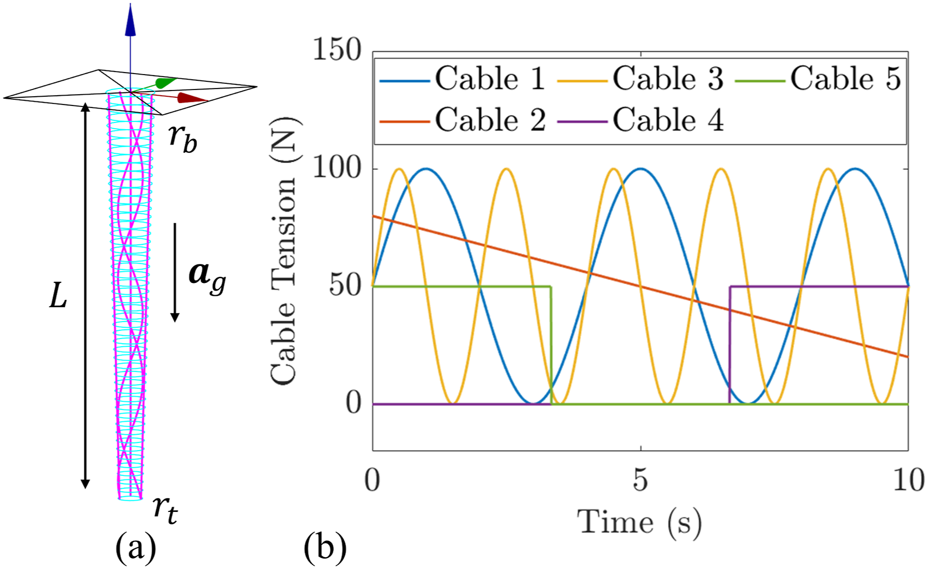
The manipulator is actuated by arbitrary time-varying inputs for 10 s, as shown in Figure 4(b). These inputs were selected to assess the robustness of the approach to different types of actuation. Specifically, the inputs for cables 1 and 3 are continuous sinusoidal functions, the input for cable 2 varies linearly, and the inputs for cables 4 and 5 consist of discontinuous step functions. We used ode15s of MATLAB as the ODE integrator, as it demonstrated the fastest computational speed for this simulation. The
Figure 5 shows the simulation results for three cases. The dynamic response is very close for all three methods. Figure 5(a) plots the states of the robot and the tip trajectory. The tip position mismatch computed using ‖Δ Dynamic response of the CDM: (a) Snapshots of the manipulator at different times and the tip trajectory with and without using analytical derivatives (AD) of FD. (b) The mismatch between the tip positions (
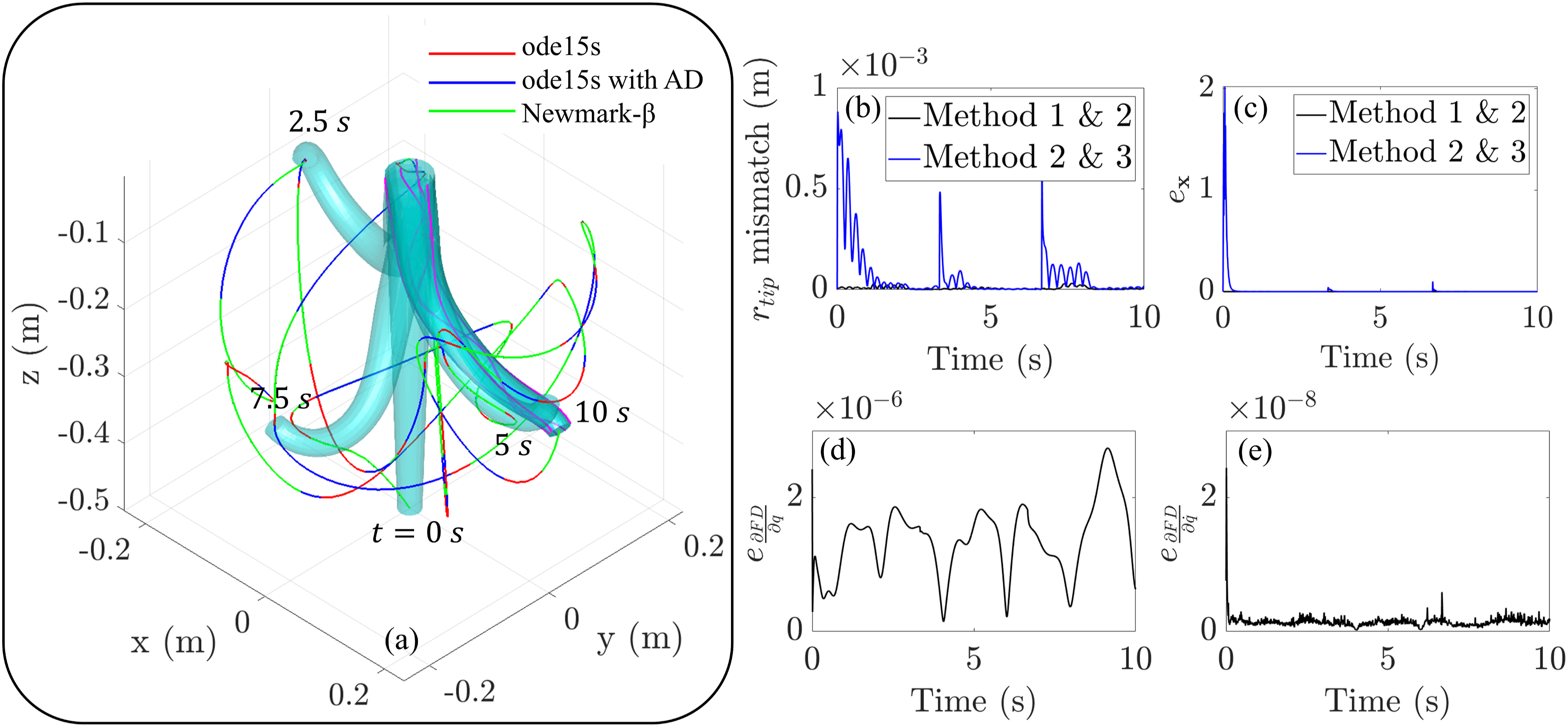
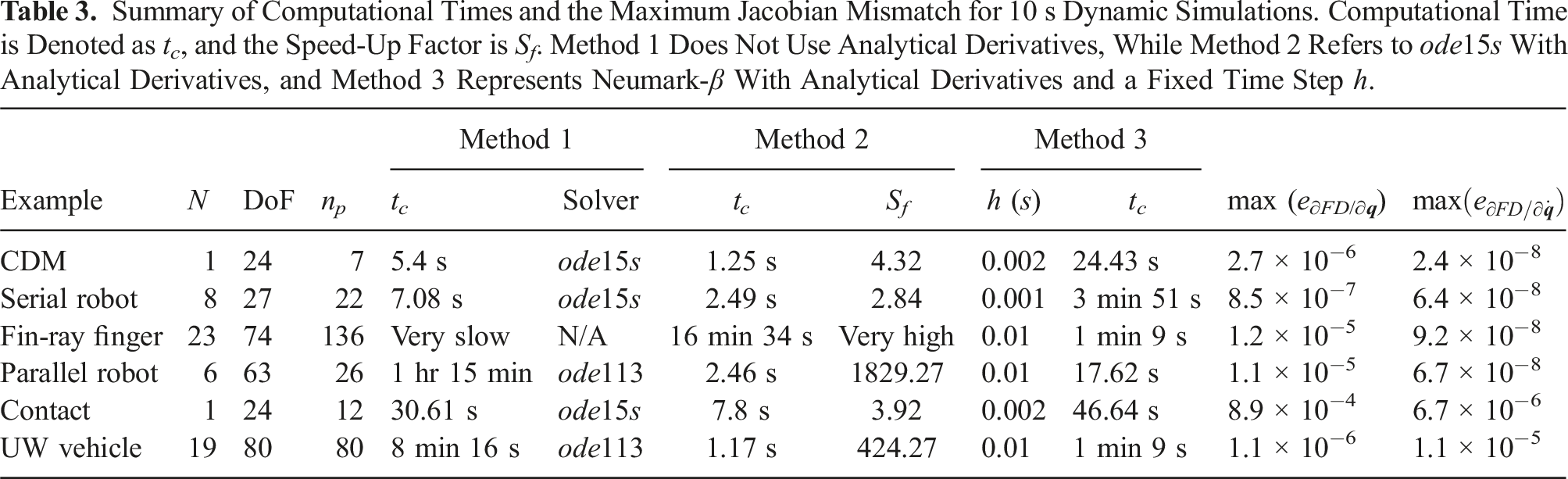
Without analytical derivatives, ode15s took 5.40 s, whereas, with analytical derivatives, it was completed in 1.25 s. This indicates that using analytical derivatives makes the computation more than 4 times faster. Simulation using the Newmark-β method was completed in 24.43 s, which can be explained by the fact that this scheme has a fixed time-step in contrast to ode15s whose time-step is adaptive.
The analytical derivatives of the forward dynamics (FD) are validated as follows. Using the finite difference method, we calculated the numerical derivatives of 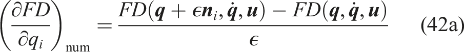
where
Using a similar metric like equation (41), we computed the mismatch between analytical and numerical Jacobian of FD with respect to 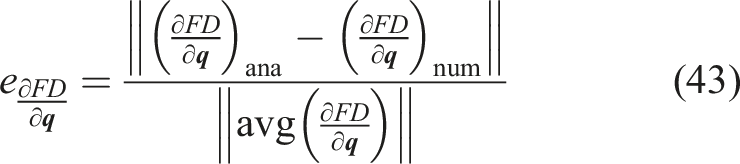
A similar equation is used for
For the static equilibrium simulation, the residue is computed using equation (17a), while the analytical Jacobian is obtained from equations (17b), (27), and (40a) with Static simulation results: (a) 10 arbitrary equilibrium shapes. (b) The mismatch between tip positions. (c) The mismatch static equilibrium solutions.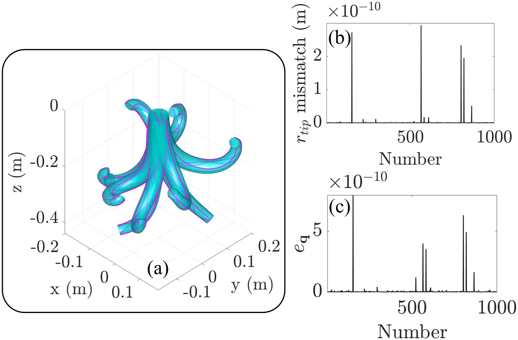
5. Extension to hybrid multi-body system
A hybrid multi-body system may incorporate rigid joints (up to 6 DoF), rigid links, soft links, branched chains, and closed-chain joints (Figure 7). The forward pass of RNEA goes through the whole multi-body (i = 1 to N) and the backward pass from i = N to 1. We propose the following rules to simplify the analysis of hybrid multi-body systems: Schematics of a generic hybrid multi-body system featuring soft and rigid links, rigid joints, branched chains, and closed-chain (CC) joints.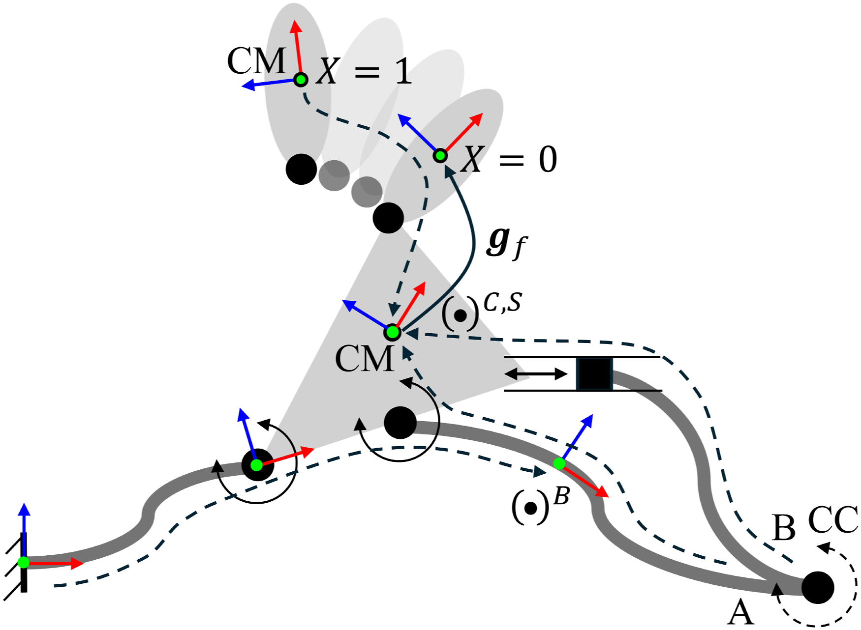
(1) Each link is defined by a rigid joint and a body (rigid or soft). Accordingly, every rigid link has two computational points: one at X = 0 and another at X = 1 of the joint. These points are defined in the body’s reference frame, typically located at the center of mass (CM), where the inertia matrix is computed. Soft links have n p + 1 computational points: at X = 0 of the rigid joint and n p along the soft body. X = 1 of the joint coincides with X = 0 of the soft body.
(2) For a rigid body, the inertial and gravitational forces act on the computational frame on the joint at X = 1. At X = 0 of a rigid joint,
(3) Let
(4) In a branched chain system, the kinematic term (•) B denotes the contribution of all joints from the global frame to the computational point α, following a serial chain. Meanwhile, (•) C and (•) S encompass all the children’s joints, including all branches ahead of point α. The dashed arrows in Figure 7 illustrate these points.
(5) Computation of (•)
B
in the forward pass follows the same rule of the geometric Jacobian in equation (2b):
Hence, while the joint quantities,
(6) Computation of (•)
S
in the backward pass follows a similar rule:
Hence, (•)
S
also has dimensions
(7) For the ith Cosserat rod, equations (25), (31), and (36) are generalized for the multi-body as follows: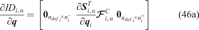
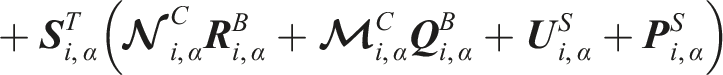
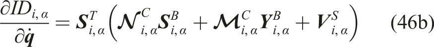
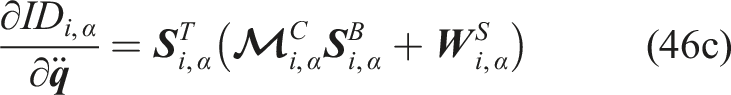
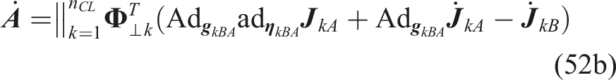
(8) Finally, the partial derivatives of ID and 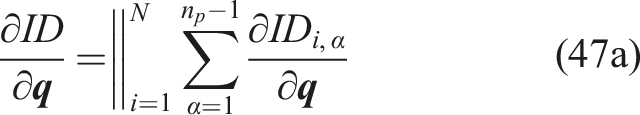
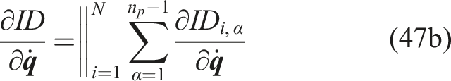
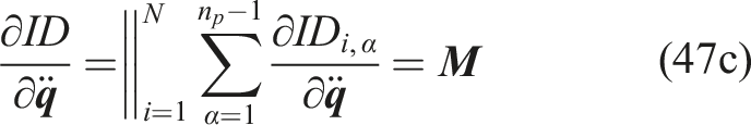
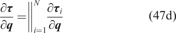
where ‖ is the vertical concatenation operator. In the backward pass from N to 1, the corresponding derivatives of each Cosserat rod (as block matrices of size
Analytical derivatives of arbitrary hybrid multi-body systems can be evaluated following these rules. In addition to these, the dynamics of a multi-body system is often subject to equality constraints that can be expressed as
5.1. Joint coordinate controlled rigid joints
Rigid joints can be actuated by specifying joint wrench
The computation of FD and its derivatives remains the same if the joint is actuated by specifying 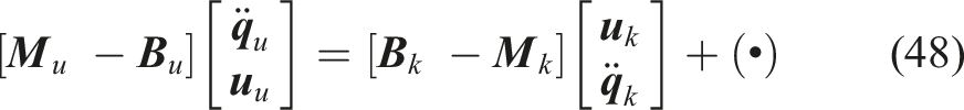
Equation (48) is used to solve 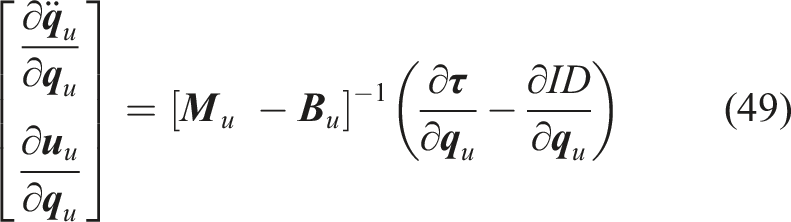
Finally, ∂FD/∂
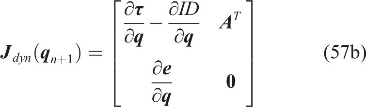
The same problem can be solved using index-3 DAE formulation using the Newmark-β scheme. In this case, we have 
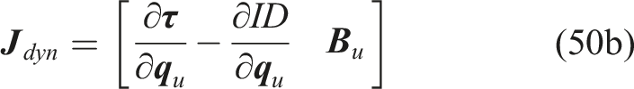
The statics problem involves finding the unknown generalized coordinates and joint forces (
5.1.1. Hybrid serial robot
We modeled a hybrid serial robot by combining a rigid serial robotic arm with a soft manipulator, as shown in Figure 8(a). The robot consists of 7 revolute joints that are actuated by arbitrary joint angles according to Figure 8(b). The actuation inputs for the joint coordinate controlled rigid joints were selected as C2-continuous functions since the joint angle, velocity, and acceleration are required for the computation of dynamics using index-1 DAE. Additionally, all joints start with an initial value of zero at t = 0. For the chosen arbitrary input, joints 1, 3, and 6 follow sinusoidal functions, joints 2 and 4 are governed by fourth-order polynomials, and joints 5 remain fixed throughout the simulation. The soft link has a fixed joint, a length of 50 cm, and a radius linearly varying from 1.5 cm to 1 cm. The mechanical properties of the soft body are identical to that of the first example. The soft body is modeled as a Kirchhoff rod (no shear deformation) with a fourth-order strain basis. Hence, in total, the robot has 27 DoF. (a) Hybrid serial robot consisting of 7 rigid links and 1 soft link with a fixed joint. The rigid links shown in red have revolute joints rotating about their local x-axis, while those in blue rotate about the y-axis. (b) Arbitrary joint angles as a function of time.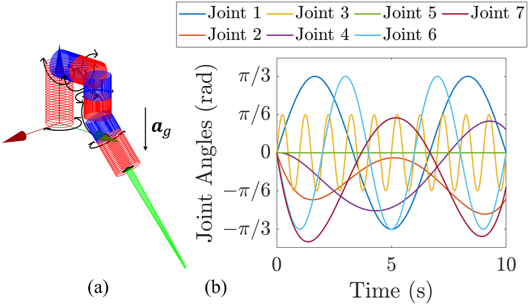
The dynamic response of the robot is computed over 10 seconds using three methods: ode15s without providing analytical derivatives, ode15s with analytical derivatives, and the Newmark-β method. For the Newmark-β approach, a time step of 0.001 s was used, as the solution failed to converge for larger time steps. Snapshots of the simulation results for the first 5 seconds are displayed in Figure 9(a). Without analytical derivatives, the ode15s took 7.08 s, while with analytical derivatives, it was completed in 2.49 s, making it approximately 3 times faster. While for our custom Newmark-β code, the simulation time was 3 min and 51 s. Mismatch metrics, similar to those in the first example, are shown in Figure 9(b)–(e). The position and state mismatch between the first two methods is in the order of 0.1 mm and 10−3, respectively. The differences between the numerical and analytical derivatives of FD indicate that their discrepancies are insignificant. Numerically computing the Jacobians took an average of 32.1 ms, whereas the analytical Jacobian required only 2.5 ms, making the analytical approach nearly 13 times faster. The mismatch metrics in Figure 9 appear noisier than those in Figure 5. This could be due to the more rapid dynamic motion of the serial robot compared to the cable-driven manipulator. Dynamic response of the serial robot: (a) Superimposed snapshots of the robot at different times and the tip trajectory with (blue) and without (red) using analytical derivatives. (b) Tip position mismatch. (c) State mismatch. The mismatch between numerical and analytical derivatives of FD (d) with respect to 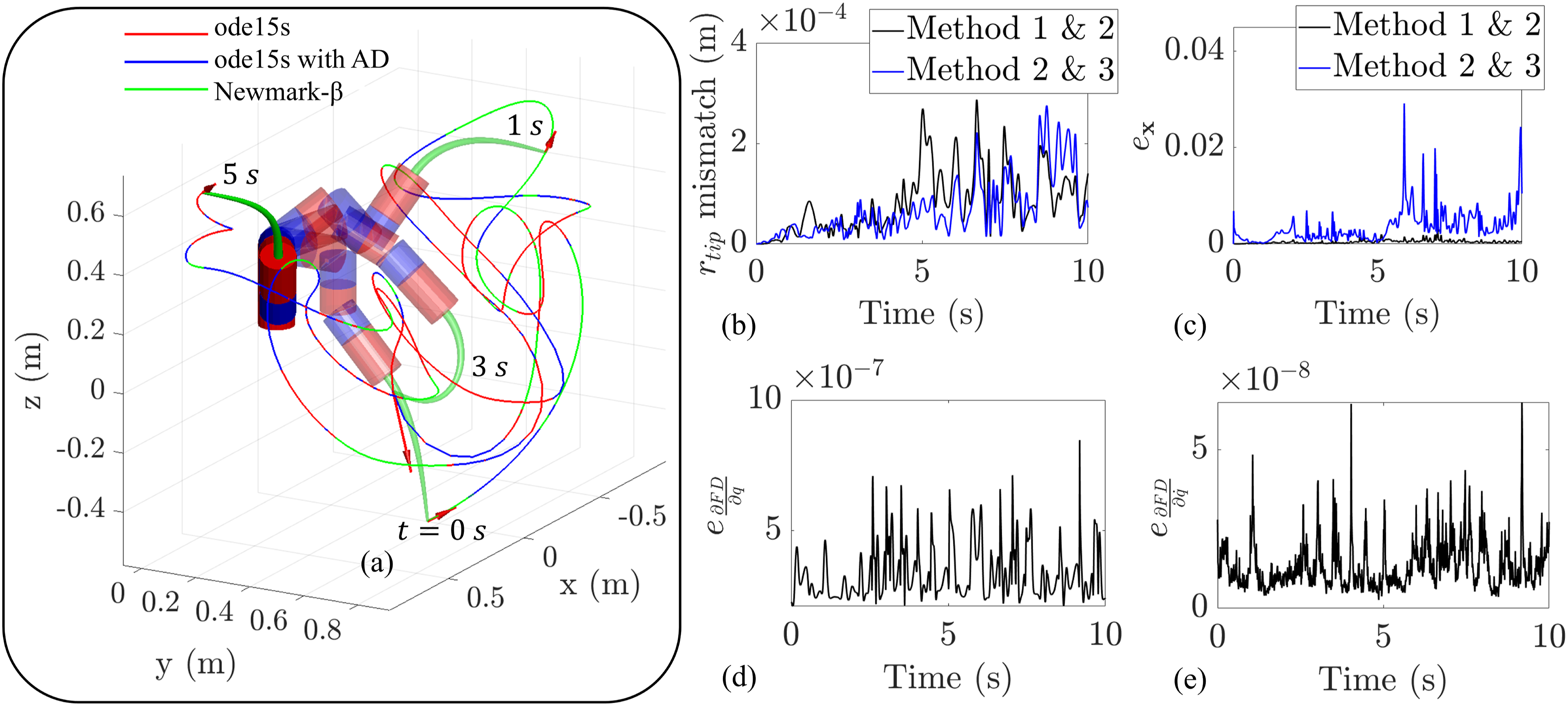
Static equilibrium simulation of the robot involves solving Static simulation results: (a) Five arbitrary equilibrium shapes, (b) the mismatch between tip positions, and (c) The mismatch static equilibrium solutions (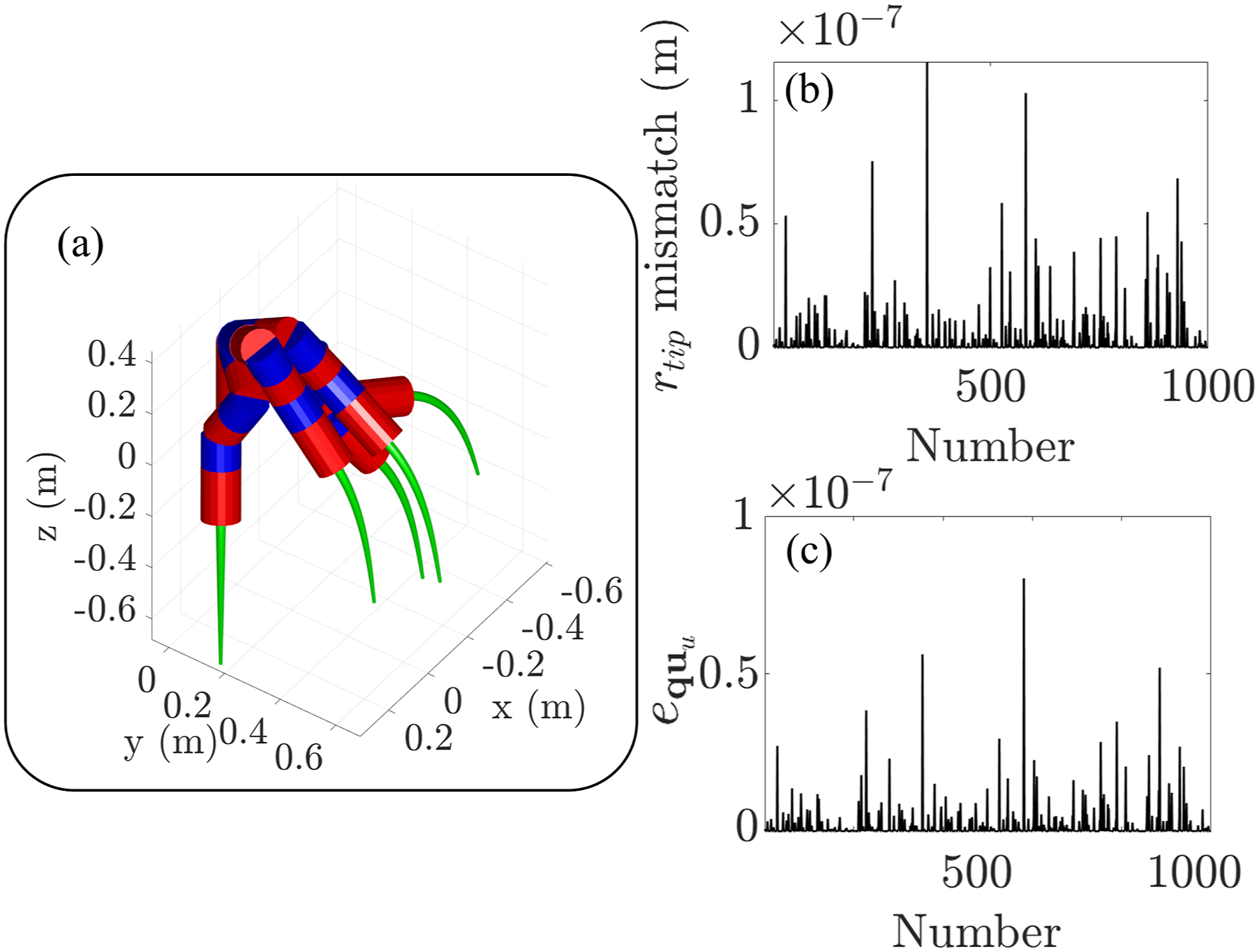
5.2. Closed-chain systems
Robots can have a closed-chain (CC) structure, as shown in Figure 7. Closed-chain systems can be modeled using kinematic constraints (
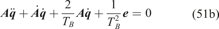
where 

where
Combining equations (51a) and (51b) we get: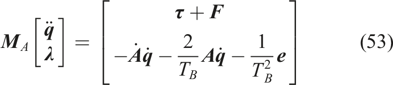
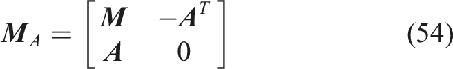
Equation (53) is used to solve for 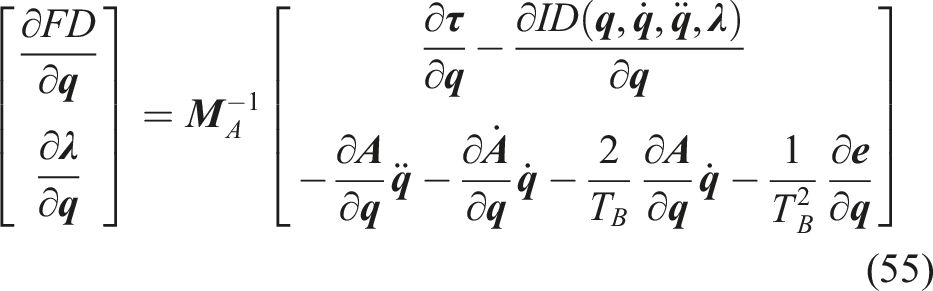
Similarly, the derivative of equation (53) with respect to 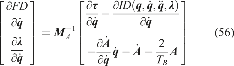
For the index-3 DAE formulation of the problem, we have additional unknowns 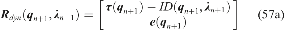
The static equilibrium simulation involves solving
5.2.1. Fin-ray finger
Figure 11 shows a fin-ray finger, a multi-body system with 17 soft links, revolute joints, a prismatic joint, and 6 closed-chain joints. The finger is actuated by a displacement of the prismatic joint, as shown in Figure 11(b). The ribs (horizontal links) are connected to the sidewalls via revolute joints. Each link has a rectangular cross-section with a width of 1 mm. The sidewalls have a height of 2.5 cm and a length of 3 cm, while the ribs have a height of 1 cm. All soft links are modeled using linear bending, constant elongation, and shear strains, resulting in a planar multi-body with 74 DoF. The material used is Acrylonitrile-Butadiene-Styrene (ABS), with a Young’s modulus of 2 GPa and a Poisson’s ratio of 0.35, commonly used in 3D printing. Five of the six closed-chain joints are revolute, and the top joint is fixed. The problem includes both the joint coordinate constraint and the closed-chain constraint. (a) A fin-ray finger with 17 soft links and 6 closed-chain joints. The robot is actuated by a prismatic joint along the global z-axis at its base. (b) Displacement input of the prismatic joint in the range −2.5 to 2.5 cm.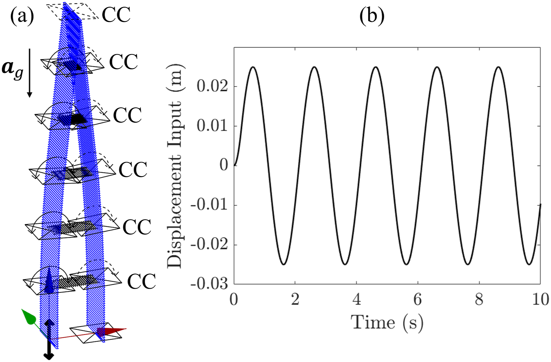
In this example, when the analytical Jacobian was not provided, the dynamics simulation using ode15s was practically stuck at 0.04 s. Other MATLAB ODE integrators, such as ode45 and ode113, progressed extremely slowly, completing only Dynamic response of the fin-ray finger: (a) Snapshots of the finger at different times with the trails of the tip position, (b) average values of mismatch between tip positions, and (c) state mismatch. The mismatch between numerical and analytical derivatives of FD (d) with respect to 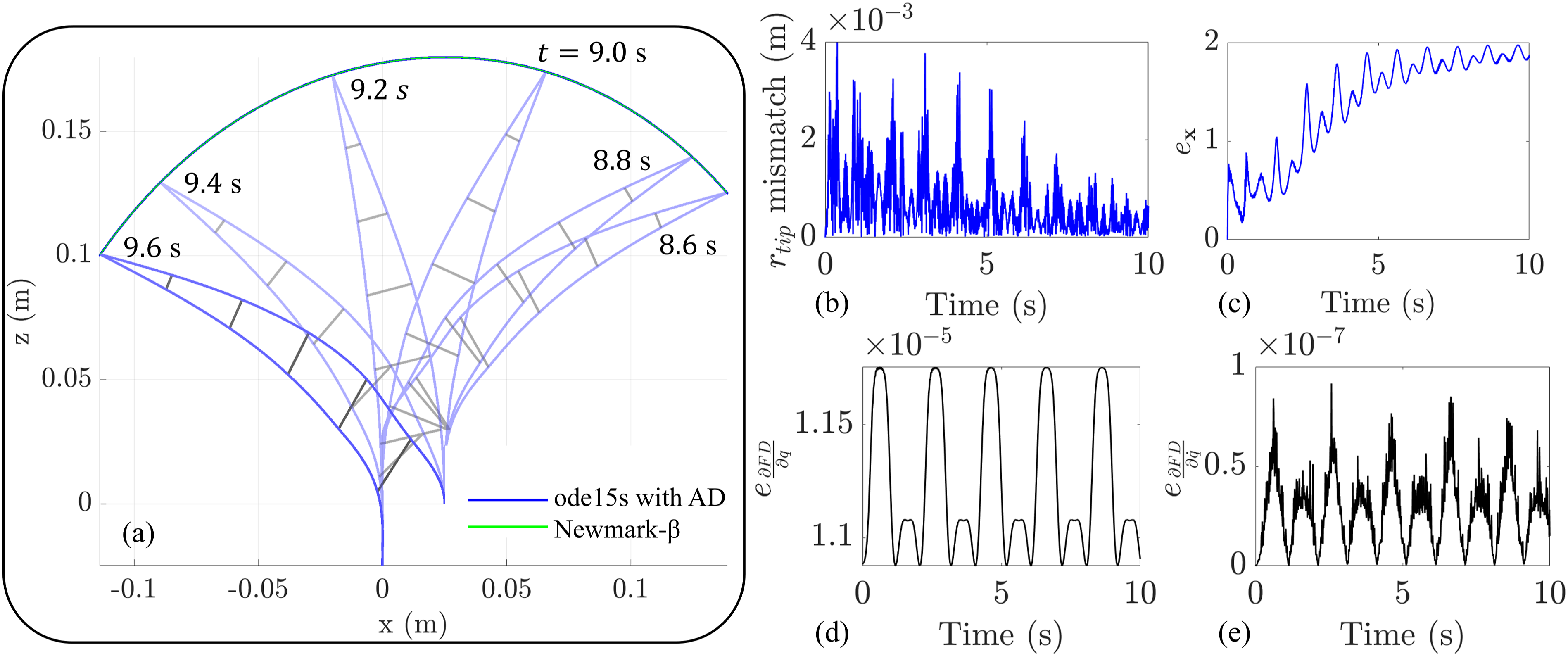
6. Examples of common external forces
In this section, we derive the analytical derivatives of various external loads to which robots are commonly subjected: point wrenches, contact forces, and hydrodynamic forces.
6.1. Point wrench
The point wrench can be expressed in the local frame (as a follower load) or the global frame. In the former case, the partial derivative of 
The derivative of this term with respect to 
Accordingly, the partial derivative of ID with respect to 
6.1.1. Hybrid parallel robot
Figure 13(a) shows an example of a hybrid parallel robot with three soft pillars and a rigid platform. The properties of the soft body are kept identical to those of CDM. The soft body is modeled as a cuboid with dimensions 1.5 cm × 3 cm × 15 cm. The top rigid platform is an equilateral triangle with a side length of 20 cm and a height of 1 cm. The soft pillars are connected to the platform via spherical joints and are parameterized using cubic angular strains and first-order linear strains. Hence, the total DoF of the robot is 63. The dynamic simulation is solved using FD computed from equation (53), with analytic Jacobians according to equations (55) and (56). The platform is subjected to an external point wrench (force and moment) in the global frame according to Figure 13(b), and the robot’s dynamic response is calculated over 10 seconds. (a) Hybrid parallel robot consisting of three soft pillars, a rigid platform with three spherical joints, and two closed-chain revolute joints subject to a point wrench (force 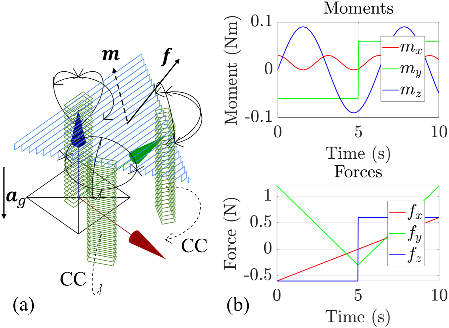
Figure 14(a) shows snapshots of the dynamic response. In this example, when the analytical Jacobian was not provided, the simulation using ode15s advanced at an impractically slow pace. Consequently, we switched to MATLAB’s ode45 and ode113 (method 1) integrators. The simulation took 1 hr 46 mins with ode45 and 1 hr 15 mins with ode113. In contrast, ode15s with the analytical Jacobian completed the simulation in just 2.46 s, making it about 1800 times faster than ode113. For the Newmark-β scheme, the computational time was 17.62 s for a time step of 0.01 s. Figure 14(b) and (c) demonstrate how closely the dynamic simulation results of all three methods align. The position and state mismatch between the first two methods is in the order of 10−5 m and 10−4, respectively. The difference between the analytical and numerical derivatives of FD, displayed in Figure 14(d) and (e), validates the analytical derivatives. Numerically computing the derivatives took an average of 82.9 ms, whereas the analytical derivatives required only 5.1 ms, making the analytical approach nearly 16 times faster. Thus, it is not just the speed of computation; its accuracy also contributed to the significant improvement in the overall computational efficiency of dynamic simulations. Dynamic response of the hybrid parallel robot: (a) Snapshots of the robot at different times with the trails of the corner positions of the rigid platform. Solid and dotted arrows indicate the applied point forces and moments, respectively. (b) Average values of mismatch between corner positions. (c) State mismatch. The mismatch between numerical and analytical derivatives of FD (d) with respect to 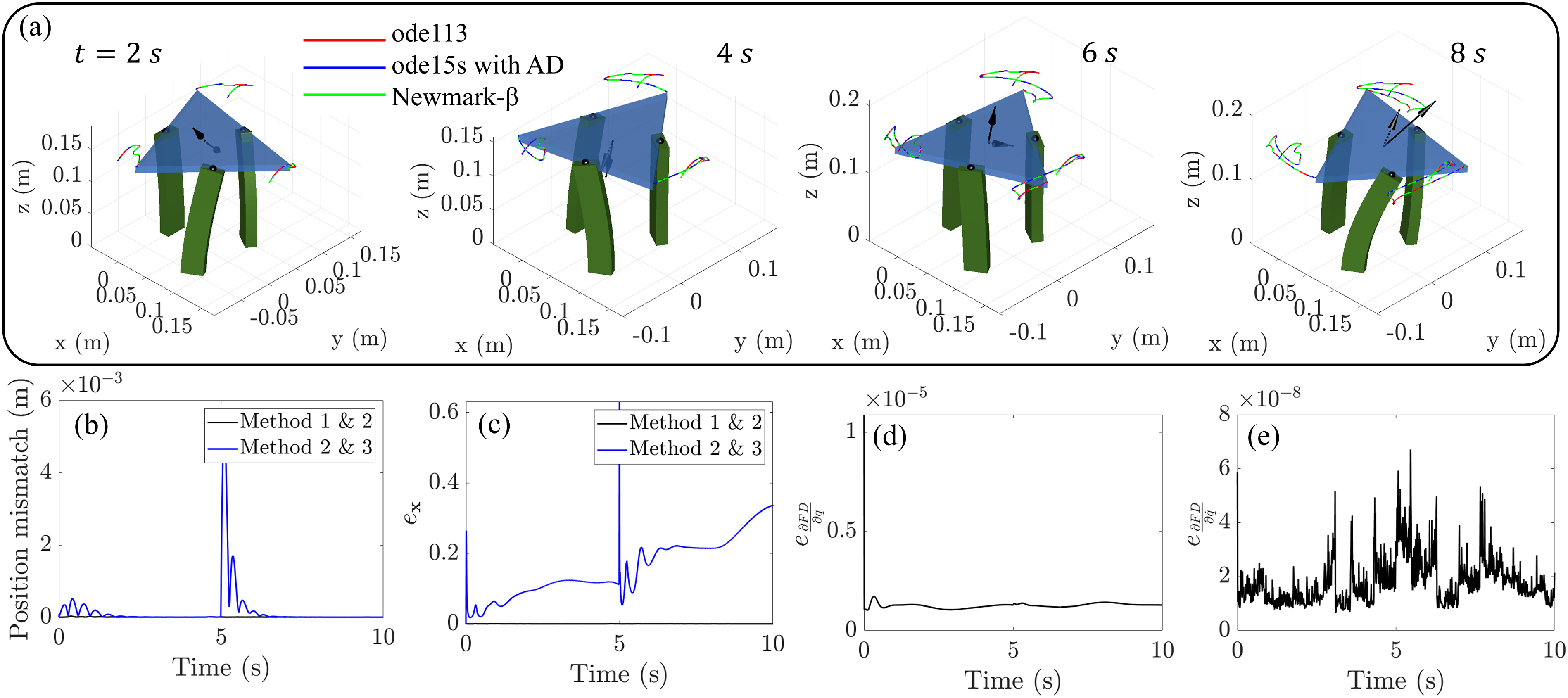
For the static equilibrium simulations, the system is subjected to 1000 randomly applied point wrenches: forces in the range −0.5 to 0.5 N and moments in the range −0.05 to 0.05 Nm. The equilibrium values of Static simulation results of the hybrid parallel robot: (a) Four arbitrary equilibrium shapes. (b) The mismatch between tip positions. (c) The mismatch static equilibrium solutions (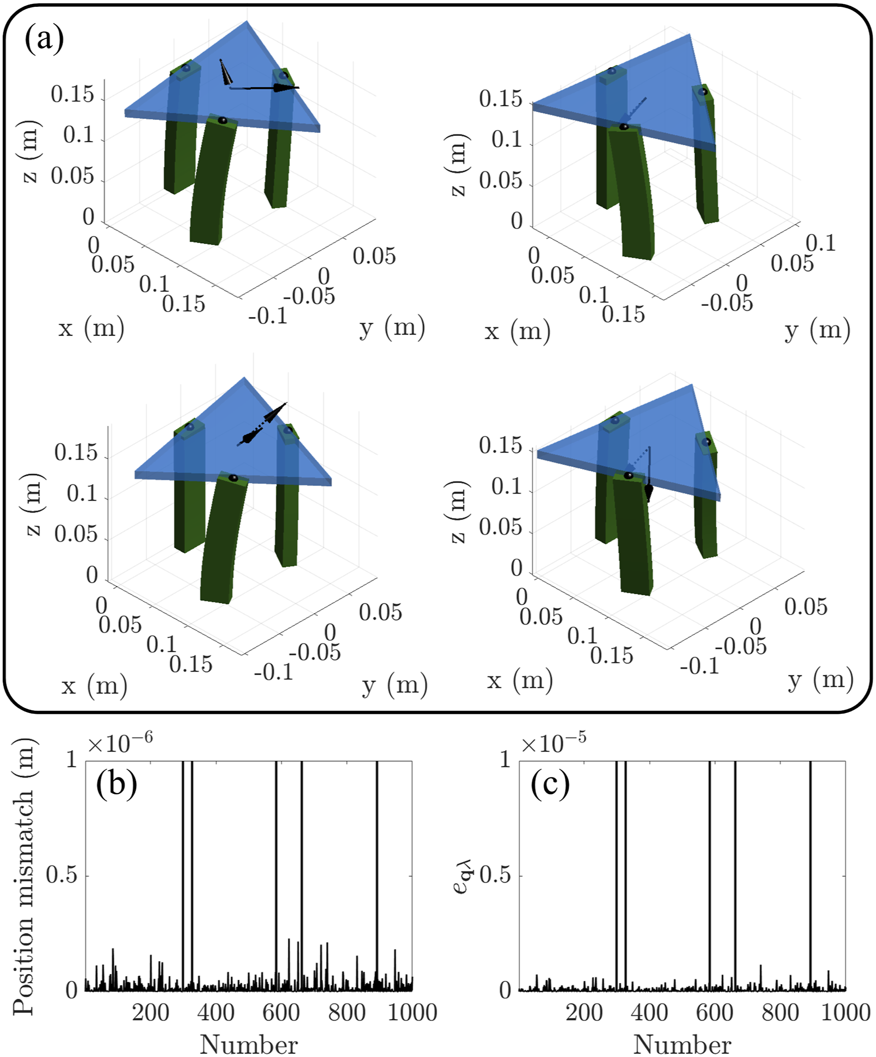
6.2. Contact force
Accurate modeling of contact mechanics is paramount in robotics and has been addressed through various models and algorithms (Lidec et al., 2024). Here, we examine a simplified internal contact scenario where a cable-driven soft manipulator, such as the one depicted in Figure 4, is actuated inside a hollow cylinder, with the cylinder’s centerline aligned to the global z-axis. The following assumptions are made to simplify the contact force: (1) To compute the contact force, the manipulator is discretized into spheres at each computational point (n
p
= 12 in this example). The radius of each sphere corresponds to the manipulator’s radius at that point k. (2) Only normal forces are considered; tangential (frictional) forces are assumed to be zero. Hence, the contact force does not cause any local moments. (3) Penetration into the cylinder is allowed, and the contact force is assumed to be a function of the penetration δ. (4) The direction of the contact force is normal to the surface of the cylindrical wall, taking the form
To model the contact force, we used the Hertz model (Flores, 2022), a two-parameter nonlinear contact model given by: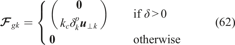

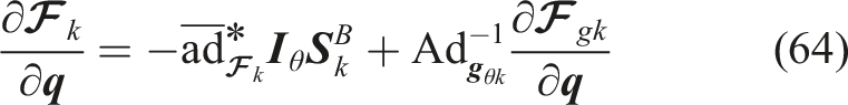
The partial derivative of the contact force in the global frame is given by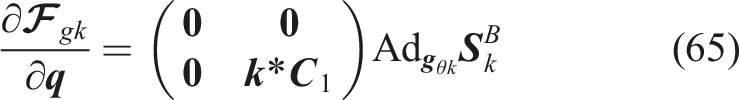

Similar to the case of point force, the derivative of the local force equation (64) is projected backward, and their contribution is accounted into the partial derivative of ID. Note that the penetration condition of the contact force equation (62) also applies to its derivative. Readers interested in detailed derivation may refer to Appendix D.
6.2.1. Contact dynamics
For the dynamic simulation, we used the same manipulator and actuation inputs as shown in Figure 4. We used an inner wall radius of r
cyl
= 15 cm, k
c
= 105 N/m, and p = 1.5. The simulation results are displayed in Figure 16(a). Simulation using ode15s without providing analytical derivatives was completed in 30.61 s, while with analytical Jacobian, it was completed in 7.80 s, making it nearly 4 times faster. Integration using the Newmark-β approach with a time step of 0.002 s was completed in 46.64 s. The validation between the methods in terms of tip position and robot state are shown in Figure 16(b) and (c), respectively. Between methods 1 and 2, the tip position mismatch is less than 40 μm and the state mismatch is in the order of 10−3. Figure 16(d) and (e) compare the derivatives of FD obtained using numerical and analytical methods. While the discrepancies are generally small, the relatively larger mismatches in the partial derivatives of FD with respect to Contact simulation results: (a) Snapshots of dynamics of CDM inside a hollow cylinder with tip trajectories. Inset showing a top view. (b) Mismatch between tip positions. (c) State mismatch. Mismatch between numerical and analytical derivatives of FD: (d) with respect to 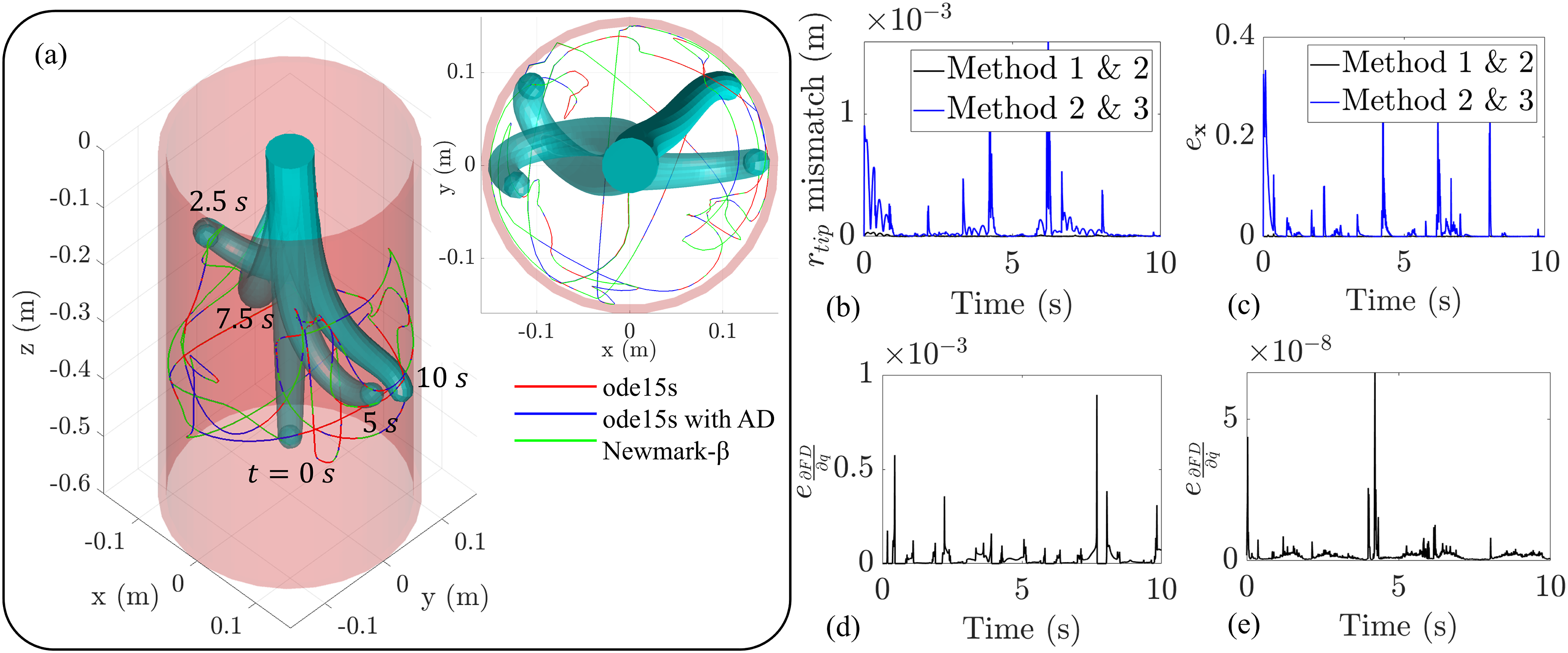
6.3. Hydrodynamic force
Several hybrid soft robots are designed for underwater exploration. In addition to gravity, they are subject to external forces due to buoyancy, drag, lift, and added mass (fluid displacement). Buoyancy acts as an acceleration opposing gravity, while the added mass force can be simplified as additional inertia that the body experiences. To model the effect of buoyancy, we can use the modified acceleration 
Substituting the partial derivative of the velocity twist (Appendix D), we get the derivative of the drag-lift force:
Similarly, we can write the partial derivative of the drag-lift force with respect to 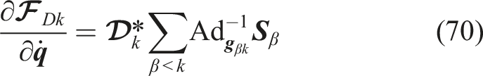
With the form of equations (69) and (70), it is easy to see that the contribution of drag-lift force can be accounted for by including an additional term in equation (24a):
6.3.1. Underwater flagellated vehicle
Using this, we simulated the dynamics of an underwater (UW) flagellated vehicle. The schematic of the robot is shown in Figure 17. The robot is a hybrid-branched chain system with a mobile (6 DoF) body, two shafts (rigid bodies with revolute joints), six soft bodies (flagella), and six hooks that connect the flagella with the shafts. The three front flagella are 35 cm long, while the rear ones are 50 cm long. Each flagellum has a base radius of 12.5 cm, tapering smoothly to a point at the tips. The material properties of the soft body are kept identical to previous examples. The robot is actuated by joint torques while subject to external hydrodynamic forces. In this example, we assume that all the bodies are neutrally buoyant (ρ
w
= ρ
b
). Each flagellum is modeled as an inextensible Kirchhoff rod with a cubic strain field, resulting in 80 DoFs for the robot. Schematic of the underwater hybrid mobile robot. The robot is actuated by joint torque and is subject to drag-lift and added mass forces.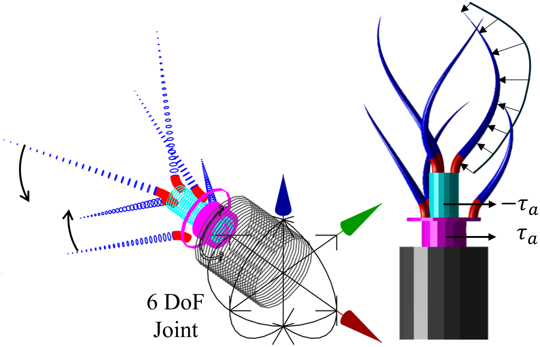
We applied a joint torque of 0.25 Nm on the first shaft and −0.25 Nm on the second to cancel out the rotation of the robot body. The dynamics of the robot are computed for 10 s. Similar to the case of the hybrid parallel robot, the simulation using ode15s without providing the Jacobian progressed very slowly. As a result, we used ode45 and ode113 (method 1), obtaining simulation times of 11 min 58 s and 8 min 16 s, respectively. In contrast, ode15s with the analytical Jacobian completed the simulation in just 1.17 s, making it more than 400 times faster. Using the Newmark-β method, the simulation was finished in 60.91s. The dynamic response of the robot is displayed in Figure 18(a). The mismatch metrics comparing the outputs of all three methods are provided in Figure 18(b) and (c). Between methods 1 and 2, the state mismatch is in the order of 10−4. The validation of the analytical derivatives of FD is provided in Figure 18(d) and (e). The numerical method took 216.4 ms on average, while the average time for the analytical approach was 11.9 ms, making it nearly 18 times faster. Dynamic response of the underwater mobile robot: (a) Snapshots of the robot at different times with the trajectory of two flagella. (b) Average values of mismatch between the tips of all six flagella. (c) State mismatch. The mismatch between numerical and analytical derivatives of FD (d) with respect to 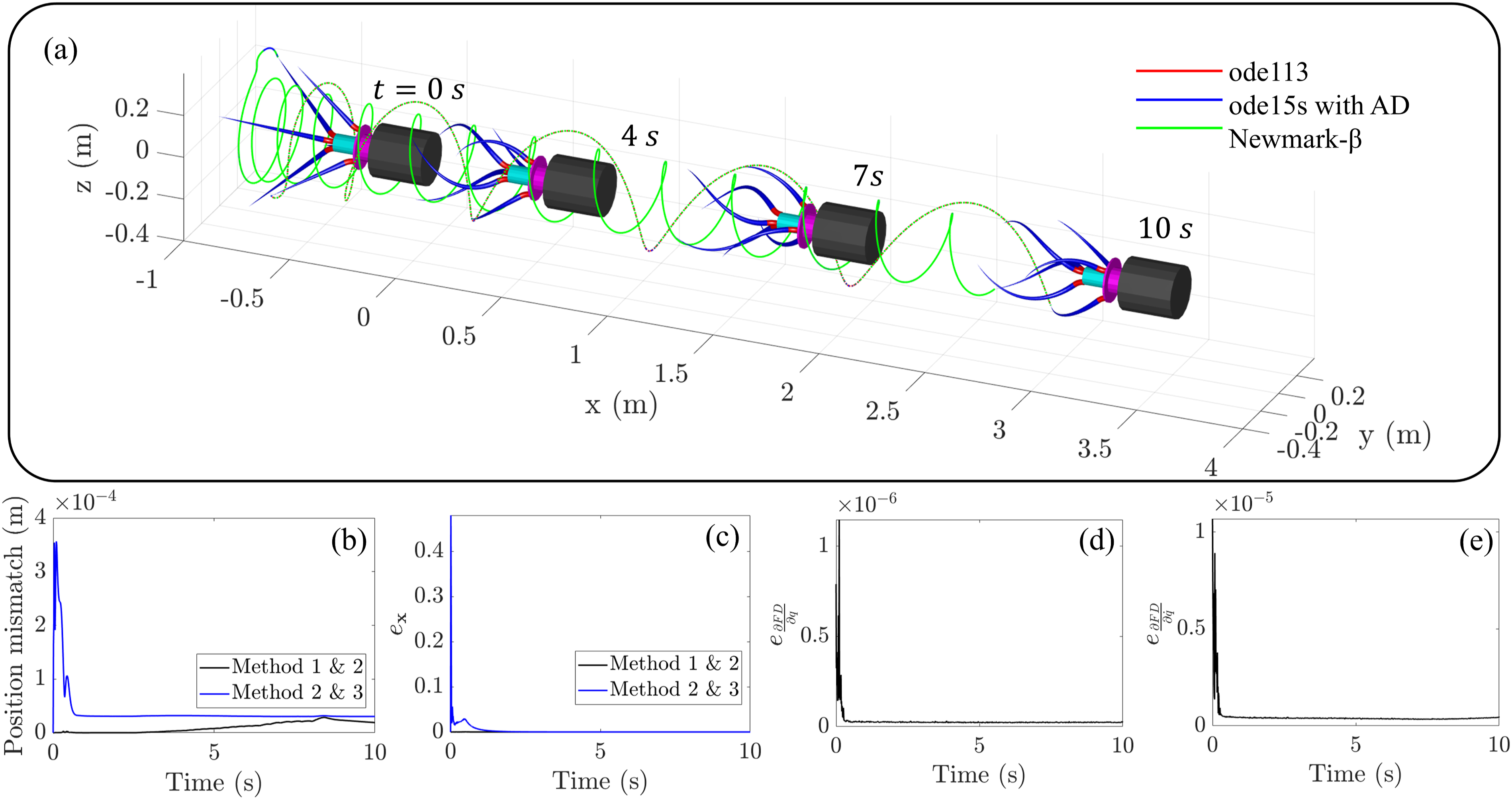
7. Discussions and conclusions
Summary of Computational Times and the Maximum Jacobian Mismatch for 10 s Dynamic Simulations. Computational Time is Denoted as t c , and the Speed-Up Factor is S f . Method 1 Does Not Use Analytical Derivatives, While Method 2 Refers to ode15s With Analytical Derivatives, and Method 3 Represents Neumark-β With Analytical Derivatives and a Fixed Time Step h.
A limitation of the ode15s solver in MATLAB is that it does not allow passing
We have implemented the GVS model in a GUI-based MATLAB toolbox called SoRoSim Mathew et al. (2022a). The toolbox allows users from various backgrounds to easily simulate hybrid multi-body systems without requiring deep expertise in underlying algorithms. Implementation of analytical derivatives for the analysis of arbitrary robotic systems is a complex task, particularly for new researchers. To further simplify this process, we updated SoRoSim into a fully differentiable simulator, using the theory presented in this work. The latest version of the toolbox can be obtained from MathWorks or GitHub Mathew et al. (2025b). The readers are encouraged to explore the toolbox and leverage its differential capabilities for various robotic analyses.
The applications of analytical derivatives extend far beyond the algorithms presented for static and dynamic analysis. They are foundational for a wide range of advanced control and optimization techniques. For example, in design optimization, they enable efficient tuning of robot geometry and material properties to achieve desired performance. In trajectory optimization, they provide efficient gradient information for motion planning, improving computational efficiency and accuracy. They are also crucial for Model Predictive Control (MPC), where real-time system predictions are needed to maintain optimal performance. Moreover, their use can significantly improve methods like Differential Dynamic Programming (DDP), especially in handling nonlinear constraints and complex robot configurations. Analytical derivatives facilitate accurate local model linearization of nonlinear system dynamics, which is essential for control design and stability analysis. They also enable sensitivity analysis by capturing system behavior changes due to parameter variations, a key aspect of robust design and uncertainty quantification. Furthermore, they enhance system identification by improving parameter estimation to minimize the sim-to-real gap. In reinforcement learning (RL), analytical derivatives aid policy optimization, accelerating convergence and improving training stability. Analytical derivatives can make several rigid-body algorithms accessible for soft robotic systems, allowing researchers to simulate and control complex hybrid systems using existing algorithms. The techniques presented in this paper offer broad applicability across the robotics field for enhancing the efficiency and precision of computations. We believe that this work will play a pivotal role in addressing challenges in soft and hybrid soft-rigid robots, driving innovation, and enabling real-world applications.
Supplemental Material
Footnotes
Declaration of conflicting interests
The author(s) declared no potential conflicts of interest with respect to the research, authorship, and/or publication of this article.
Funding
The author(s) disclosed receipt of the following financial support for the research, authorship, and/or publication of this article: This work was supported by the Khalifa University of Science and Technology under Grants RIG-2023-048 and RC1-2018-KUCARS, as well as the French ANR COSSEROOTS (ANR-20-CE33-0001).
Supplemental Material
Supplemental Material for this article is available online.
Appendix
References
Supplementary Material
Please find the following supplemental material available below.
For Open Access articles published under a Creative Commons License, all supplemental material carries the same license as the article it is associated with.
For non-Open Access articles published, all supplemental material carries a non-exclusive license, and permission requests for re-use of supplemental material or any part of supplemental material shall be sent directly to the copyright owner as specified in the copyright notice associated with the article.