
Abstract
Modeling soft robots is not an easy task owing to their highly nonlinear mechanical behavior. So far, several researchers have tackled the problem using different approaches, each having advantages and drawbacks in terms of accuracy, ease of implementation, and computational burden. The soft robotics community is currently working to develop a unified framework for modeling. Our contribution in this direction consists of a novel dimensionless quantity that we call the softness distribution index (SDI). The SDI for a given soft body is computed based on the distribution of its structural properties. We show that the index can serve as a tool in the choice of a modeling technique among multiple approaches suggested in literature. At the moment, the investigation is limited to bodies performing planar bending. The aim of this work is twofold: (i) to highlight the importance of the distribution of the geometrical and material properties of a soft robotic link/body throughout its structure; and (ii) to demonstrate that a classification based on this distribution provides guidelines for the modeling.
1. Introduction
Soft-bodied robots are often counterposed to rigid-linked robots. The former have gained huge popularity in recent years; the field is relatively young and since its appearance it has posed many challenges to researchers (Laschi et al., 2016; Lipson, 2014; Rus and Tolley, 2015). The latter belong to an older, deeply investigated field, in which researchers have solved major problems related to design and control; as a result, rigid-linked robots have found several industrial applications, in which both serial and parallel manipulators are used to perform various tasks, such as pick-and-place operations and handling of heavy metal sheets, at high speed and with high accuracy and precision.
Rigid-linked robots are usually provided with variable stiffness joints and actuators (Wolf et al., 2016), which improve the performances at the cost of increased complexity in the control. In these systems, named articulated soft robots, the joint stiffness is treated as a lumped parameter (LP), as explained by Albu-Schäffer and Bicchi (2016). In addition to the stiffness of the joints, the stiffness of the robotic links is taken into account in the study of elastodynamics: the eigenfrequencies of a manipulator depend on the structural properties of all its parts, and on how such parts are interconnected. Correct estimation and appropriate modeling of the stiffness of a robotic system are crucial to avoid undesired vibrations, which may jeopardize the performances in operative conditions. Therefore, the topic has been addressed by several authors in their works (to mention a very few of them, Pashkevich et al. (2009), Briot et al. (2009), Cammarata (2012), Zhang et al. (2015), Germain et al. (2015), and Rognant et al. (2010)). If the modeling of the stiffness plays such a key role for the so-called rigid-linked robots, it is easy to figure out that its importance is even greater for soft-bodied robots: in fact, they rely upon their low stiffness to perform a task, adapting their shape to the surrounding environment, often elegantly.
Unfortunately, the beauty of soft robots is also the beast that researchers have to fight. Different approaches have been proposed to tackle the problem of modeling soft-bodied robots. Among the most popular, we find the use of the finite element method (FEM). In fact, some authors use finite element commercial software to evaluate the mechanical response of their soft robots and actuators, to perform structural optimization or to develop their optimization method based on finite element simulations (e.g., Connolly et al., 2015; Elsayed et al., 2014; Moseley et al., 2016; Polygerinos et al., 2013; Runge et al., 2017; Suzumori et al., 2007). When using FEM, the stiffness appears in the so-called stiffness matrix, the size of which depends on the number and the kind of elements used. The computation of the inverse of this matrix is often a bottleneck: finite elements are indeed a powerful tool, but they come at a high computational cost. For this reason, other authors have implemented their own finite element code to make it suitable for real-time simulations; such huge work has required the efforts of a team and is part of a bigger framework (SOFA) presented in literature some years ago (Faure et al., 2012), followed by papers that expanded the work and prove its validity (such as Duriez, 2013; Ficuciello et al., 2018; Largilliere et al., 2015).
Other researchers based their approach on the Cosserat rod theory (Renda et al., 2017, 2014, 2018). In these works, the authors modeled the stiffness of soft bodies by means of a diagonal stiffness matrix; in some case, they discretize the structure of the body along its longitudinal axis and write a stiffness matrix for each segment. Recently, Grazioso et al. (2018) proposed a geometrically exact model that combines Cosserat rod theory and finite elements; in this work, as well as in previous approaches (such as that of Grazioso et al., 2016), the authors account for the stiffness by the same diagonal matrix. These works concern the modeling of continuum arms, that is, slender structures that can be discretized as a series of rods or beams.
Different approaches have also been found. For instance, some recur to the classical beam theory (Shapiro et al., 2015) or they start from the computation of the elastic strain energy (Connolly et al., 2017) to model soft pneumatic actuators, or use the elastica theory (Armanini, 2018; Armanini et al., 2017; Zhou et al., 2015) to describe the behavior of soft links to be used for soft robotics applications. Finally, some researchers do not develop any structural model for their soft robots. In these cases, the approach is purely experimental and the design and the development of the soft-bodied system is based on intuitions and qualitative considerations, and improved by trial and error.
All the approaches recalled above have both advantages and limitations in terms of accuracy, required computational burden, ease of implementation, and applicability. Researchers agree that the field still lacks a unified framework for modeling (Renda et al., 2017; Trimmer et al., 2015), and, more in general, that the development of a common approach for modeling, design, and control will be crucial for the success of the field (Bao et al., 2018). Despite the relevant progress in recent years, modeling soft robots still remains a challenging task. The difficulties lie in their highly nonlinear mechanical behavior. A first source of nonlinearity is geometrical and comes from the fact that they typically undergo large deflections, and in some cases, large strains. A second, no less important, source may come from the materials often used to build the body of the robot: polymers are characterized by nonlinear stress–strain curves, whose trends are captured by well-established models (e.g., Arruda and Boyce, 1993; Mooney, 1940; Ogden, 1972). Owing to the use of these materials (in addition to colloidal and granular matter), Wang and Iida (2015) used the term soft-matter robotics to highlight the role played by the material properties. In our opinion, there is a further aspect to consider: two soft bodies can behave very differently in terms of deformed shape, even though they are built with the same material, have the same size and undergo large displacements of the same order of magnitude, under the same external load. Very roughly speaking, some soft links can be considered more hyper-redundant than others.
In this article, we do not propose any new modeling technique. Instead, we explain why and how we have taken a step back and analyzed the problem of modeling soft-bodied robots under a different light. The focus of our work is not only on how soft a robotic link is, but also, and in particular, on the distribution of its structural properties, and on the role that such distribution plays when a modeling technique must be chosen among others. To refer to the distribution in a quantitative way, we define what we call the SDI for planar bending. We show that this index, which is a complex number, allows classes of soft bodies to be associated with one or more modeling techniques involving different numbers of parameters (and, therefore, having different computational cost).
To better share our view with the reader, we present the work following the stream of ideas and considerations that have led us to the results here reported. Therefore, Section 2 provides a discussion about stiffness and softness, from which we have found motivation for our work. Section 3 introduces the SDI. In Section 4, we briefly recall the modeling techniques that we use in this work, and that we relate to ranges of value of the index. Section 5 reports the study performed on a class of bodies, modeled by the techniques listed in Section 4; to complete the investigation, other bodies with particular distribution of the structural properties are considered in Section 6. In Section 7 we report few examples that show how the SDI can be used when performing optimization of a structure performing bending under a set of applied loads. Section 8 contains a discussion concerning the usefulness of the proposed index and highlights possible applications. The limitations of the current work are also clearly stated, to not mislead the reader. Conclusions follow.
2. Stiffness and softness
Stiffness is a property of structures and it depends on both the material and the geometry. It is a physical quantity defined in relation to an applied load and the consequent deflection along the considered direction; it is indeed a relative quantity. By the term soft we refer to a body, robot, or structure, having low stiffness. In this article, therefore, we often use the term softness as complementary to stiffness. By the term rigid, instead, we refer to a body having much greater stiffness than that of the surrounding environment (as is well known, the definition of rigid body is purely the result of abstraction).
2.1. Stiff or soft?
Let us now consider two systems: one made of two rigid links connected by an elastic rotational joint, counterposed to a single soft link. The difference between the two is clear: in the former, the compliance is localized at the joint; in the latter, the compliance is distributed and the relative position between the two end sections depends on the position and orientation of all the intermediate sections. Therefore, the compliance of the former can be modeled by one parameter, treating the joint as a torsional spring; for the soft link, such approach generally turns out to be inapplicable. These two examples represent the extrema of the path depicted in Figure 1: it is possible to consider infinite systems between these two, with gradually more and more distributed compliance. Indeed, one may ask whether there is precise, sharp boundary between what is soft and what is rigid, along this path. We all distinguish soft robotic links from rigid links based on our intuition, but can we draw a sharp line that separates these two classes?
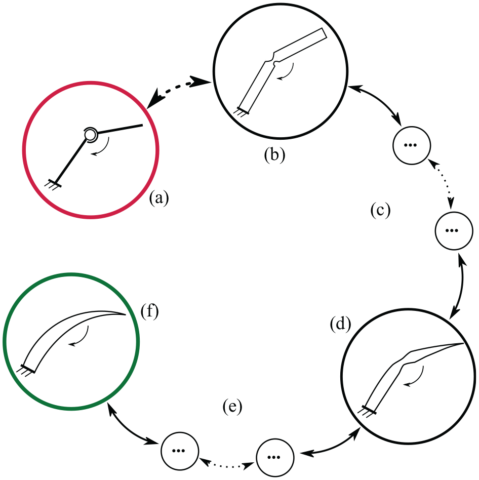
From rigid to soft robotic system, passing through intermediate systems with gradually distributed compliance, and viceversa. The dashed arrow represents the giant leap from a rigid system provided with a rotational joint (a) to a continuum, compliant system (b). Full arrows denote the transformation from (b) to continuum systems such as that in (d) passing through an infinite number of systems (c) in which the structural properties are more and more uniformly distributed; continuing with this transformation (e), the final result is a continuum, soft link (f) unequivocally. The same reasoning applies in the reverse way: from the distributed compliance of system (f), systems with more and more concentrated compliance are obtained up to the hinge-like mechanism (b), and a final giant leap consists of jumping to the non-continuum rigid-linked robot (a).
A similar question was posed by Ananthasuresh (2013) about differences and similarities between compliant mechanisms (CMs) and rigid-body mechanisms (RBMs). In this work, Ananthasuresh highlighted that CMs have features in common with both RBMs and stiff structures: because they are continuum systems they can be seen as structures; at the same time, they do not differ from RBMs in terms of function as well as of modeling approach. In fact, the pseudo rigid-body model (PRBM) has been proposed (Howell and Midha, 1995; Howell et al., 1996), by which the continuum structure of the CM is transformed into its equivalent RBM with lumped springs. Later, Cao et al. (2015) proposed a unified synthesis approach without any prescription of the type of mechanisms obtained.
2.2. How to choose the modeling technique
CMs usually consist of thin leafsprings with uniform cross section or in relatively rigid rods connected by flexural pivots that provide mobility to the mechanism. As explained by Ananthasuresh (2013), in some cases finite elements are needed to model the mechanical response of the CMs to applied loads, especially if an accurate analysis of the mechanical stress must be performed. However, the PRBM well describes the deformation of most of the CMs and other CMs are studied by a spring–mass–lever (SML) model. An important remark is that models such as the PRBM and the SML are useful for synthesis purposes (e.g., Howell and Midha, 1994, 1996; Pucheta and Cardona, 2010). Therefore, the choice of a modeling technique is not merely a matter of convenience in terms of computational burden and accuracy; it also helps in synthesis, optimization, and to achieve a deeper understanding of how the system works. There is no reason to believe that these considerations do not hold for soft-bodied robots too.
In general, the bodies that constitute a soft robot can have irregular geometry and can be made of multiple materials. To provide a few examples, the actuator by Elsayed et al. (2014) and the soft tentacle by Martinez et al. (2013) are made of more than one polymeric rubber; the soft finger developed by Manti et al. (2015) has irregular geometry and is made of two materials; the robot that appears in the work by Largilliere et al. (2015) is a parallel machine whose soft limbs have variable cross section along their length. All these systems are capable of large displacements, but they differ in that they exhibit different deflected configurations under the same applied load. Some distributions can be effectively described by models based on few parameters, as happens for some CMs; others require more computationally expensive techniques. As the deformation of a body strongly depends on both the structural properties and their distribution, it seems useful to consider not only how soft a system is, but also how the softness is distributed throughout it, to select a modeling technique that describes the deformed configuration with the required accuracy and at the lowest computational cost. Let us consider again that a compliant link with a flexural pivot (such as that in Figure 1(b)) can be transformed into one with uniformly distributed compliance (such as that in Figure 1(f)) by a continuous transformation of its structure; if we cannot draw the aforementioned line that separates soft bodies from rigid bodies, how can we assess to what extent the methods developed for rigid-linked robots and CMs can be used for soft robots? It is worth investigating this aspect, to try to draw this line and provide quantitative, rather than qualitative, answers.
Therefore, we need a quantity that takes into account the variation of the structural properties along a given direction in the system. In the next section, we define such quantity and we discuss its meaning. As a considerable number of soft-bodied robots (such as soft continuum manipulators, soft fingers) perform their tasks by bending, the definition is based on this deformation mode.
3. SDI for planar bending
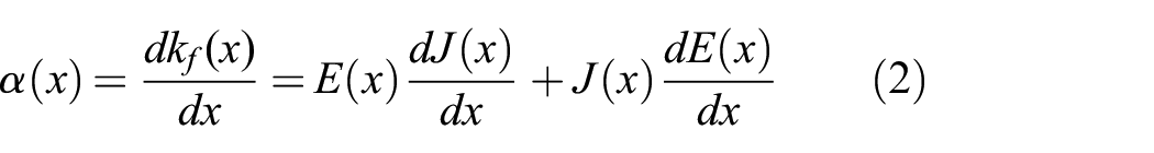
As already stated, a soft robot body can have irregular geometry and can be made of multiple materials. Figure 2 represents a beam in which both the cross section and the material properties vary along the longitudinal axis. Denoting by

where
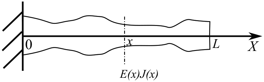
Beam with variable cross section and material along the longitudinal axis
Provided that
We denote by

where it is
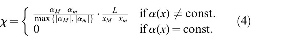
and
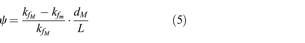
in which
The real part of the SDI accounts for the distribution of
The SDI can be computed for any body
From now on, the objective of the work will be to find a correlation between a body
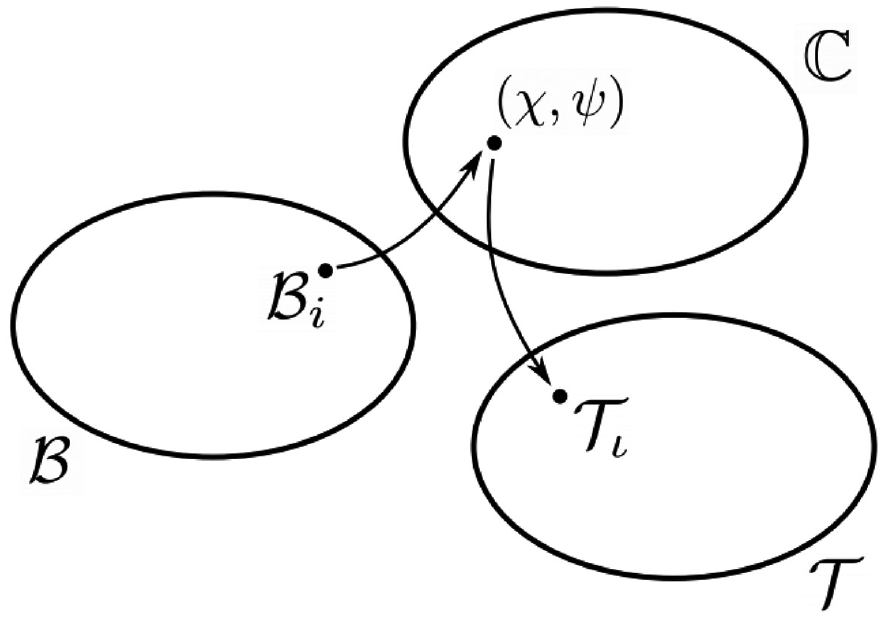
The SDI associates the body
4. Modeling techniques
As already stated, we consider four different approaches/techniques to study the static mechanical response of bodies:
finite element analysis (FEA);
nonlinear matrix structural analysis (NMSA);
elastica approach (EA);
LPs model (LPM).
In the following, we briefly recall these techniques and we explain why they have been selected among others for the purpose of this work. To avoid cumbersome mathematical expressions and excessively long discussion, the details are reported in the appendices at the end of the article, when needed.
4.1. Finite elements
In structural analysis, finite elements (FE) allow mechanical systems to be studied, however complex; that is, having irregular geometry, multiple materials, under any boundary conditions included distributed loads and occurrence of contact. They have been widely used in the last 60 years for a variety of engineering problems in which analytical models would be extremely difficult to handle, if not unworkable. The effectiveness and the consequent popularity of the method has led to the implementation of both commercial and open-source software, employed worldwide for analysis and optimization. To summarize, the method is based on the discretization of the investigated system in a number of elements having finite dimensions; the result of the discretization is called a mesh. For the generated mesh, a set of algebraic equations are written that correlates the vector of nodal displacements to the vector of nodal forces by means of the stiffness matrix.
A review on the topic goes far beyond the scope of this paper; we limit the discussion to the description of the settings adopted using a commercially available software (ABAQUS®). In all the performed simulations, the type and the number of elements has been selected in order to obtain reliable results. For each simulation, we have verified that no excessive distortion of elements had occurred and that a further increase of the fineness of the mesh did not lead to any significant change in the results obtained. Moreover, for the purpose of this work, all the simulations account for large deflections.
It is necessary to remark that in this work we do not implement a FEM model that needs to be validated, nor do we suggest the use of FEM as a general approach; our aim is to compare the results of FEA with those obtained by other techniques that involve far fewer parameters. From now on, therefore, we consider the deformation computed by FEA as the most accurate, but at the highest computational cost.
4.2. NMSA
Matrix structural analysis (MSA) can be considered the mother of the well-established FEM. For the interesting story of this technique and the way it finally turned into FEM, the reader can refer to Felippa (2001). Applications of the technique can be found in works addressing the elastodynamics of conventional rigid-linked manipulators (such as those cited in Section 1).
As stated previously, for the purposes of this work, we analyze soft bodies performing planar bending. Similarly to FEM, the body is discretized into a certain number of elements having finite dimensions; in this work, we use two-node beam elements, each node having three degrees of freedom (DOFs) on the plane (the translations along two orthogonal directions and the rotation along the axis orthogonal to the plane). As a result, each element is characterized by a
A complete and detailed explanation of the method can be found in McGuire and Gallagher (1979). To model the dynamics of a system, a mass and a damping matrix are also defined; however, our investigation is limited to the static response of bodies. Therefore, when using MSA we will write the stiffness matrix only.
If the assumption of small displacements is valid, nodal displacements and nodal forces are related by the very well-known Hooke’s law, that is, by a linear relation. To account for large displacements, NMSA must be carried out. For this reason, in this work we implement a linear-incremental MSA: the external load is applied in incremental way in a predefined number of steps. Although each step is linear, the overall computation is nonlinear, because at each step the stiffness matrix is updated based on the displacements computed in the previous step. A detailed mathematical description is reported in Appendix B.
4.3. EA
Some authors have investigated the use of the EA to model the mechanical response of soft links or arms (Armanini, 2018), suggesting potential application in the field of soft robotics. Unlike FEM and MSA, which are based on algebraic equations written in matrix form, this approach involves differential equations. A brief discussion on the topic can be found, for instance, in Howell (2001).
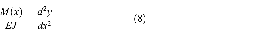
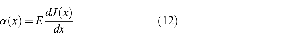
The theory allows to account for large deflections of a beam subject to an applied load; the relation between the curvature and the bending moment is described by the equation
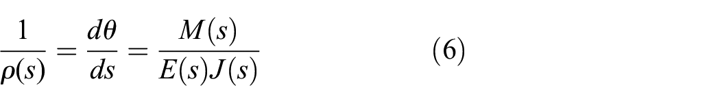
in which
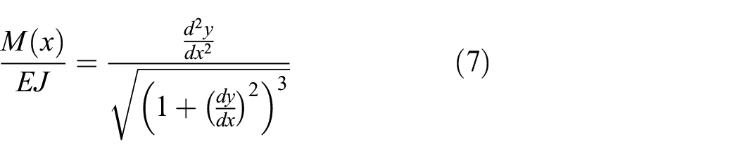
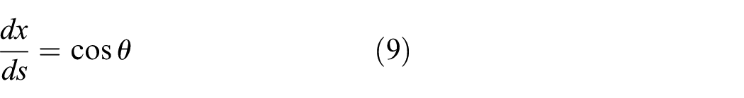
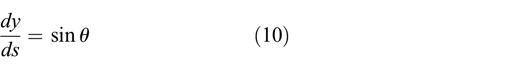
For a beam undergoing small deflections, the derivative
and it can be integrated twice over the length of the beam to compute the vertical deflection
The integration of Equation (6) may be a difficult task, depending on the loading and constraint conditions. In general, the equation is reworked, written in a form that contains elliptic integrals and solved by numerical techniques (see, for instance, Zhang and Chen, 2013).
4.4. LPs
LPs are used in a huge variety of domains other than robotics, such as the automotive industry, civil engineering, and biomechanics.
The advantage of using LPs is the low computational cost, especially compared with other techniques such as FEM. A lumped stiffness
However, in many cases LPs turn out to be insufficient to describe the deformed configuration of a system: for instance, the variable radius of curvature of a long, soft continuum arm that performs bending would be scarcely captured by few lumped springs.
In the following section, we model the planar bending of a body using few parameters, whose values are computed based on the structural properties.
5. A soft notched body made of uniform material
Keeping in mind the concept depicted in Figure 1, our investigation starts with a soft notched body made of one material having Young’s modulus
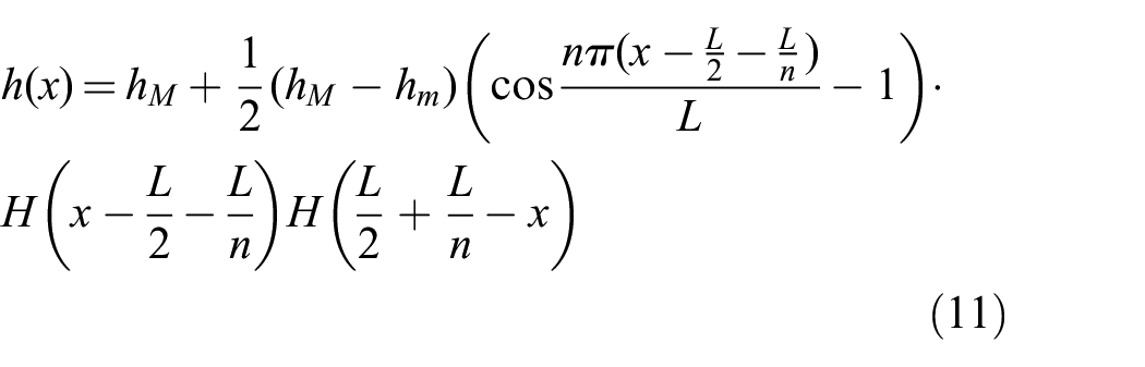
in which
Notched soft body made of one material and with variable cross section along the
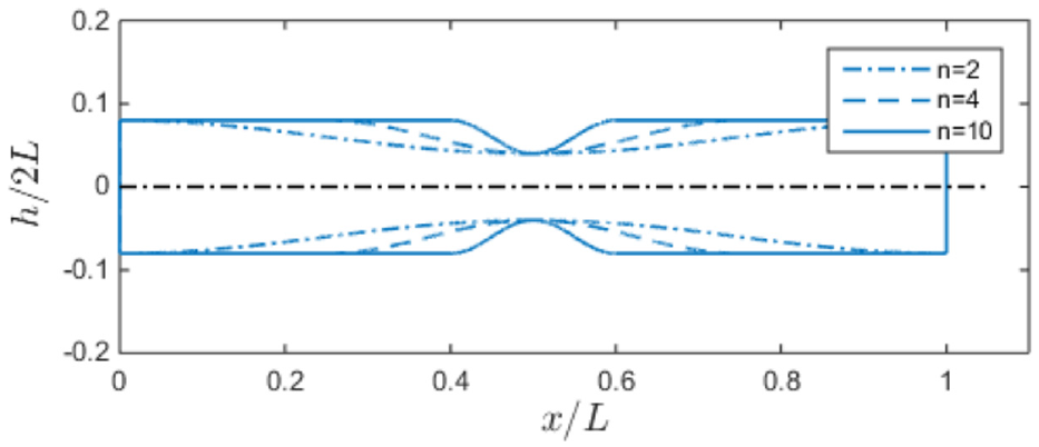
Bodies with variable cross section characterized by different
Therefore, in this section we speak about the variation of
By tuning the parameter
In this section, we compute the SDI for this class of bodies, we model the bodies by using the modeling techniques listed in Section 4 and, based on the results obtained, we derive the correlation between the SDI and the convenience of a modeling technique in terms of accuracy, computational burden and ease of implementation.
5.1. SDI for the notched body
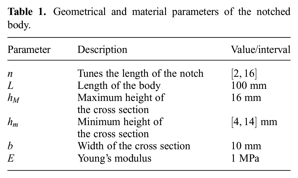
The SDI as defined in Equations (3), (4), and (5) depends on
Geometrical and material parameters of the notched body.
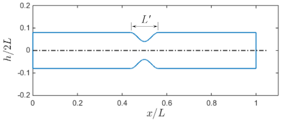
To provide an example, Figure 6 shows the graph of the function
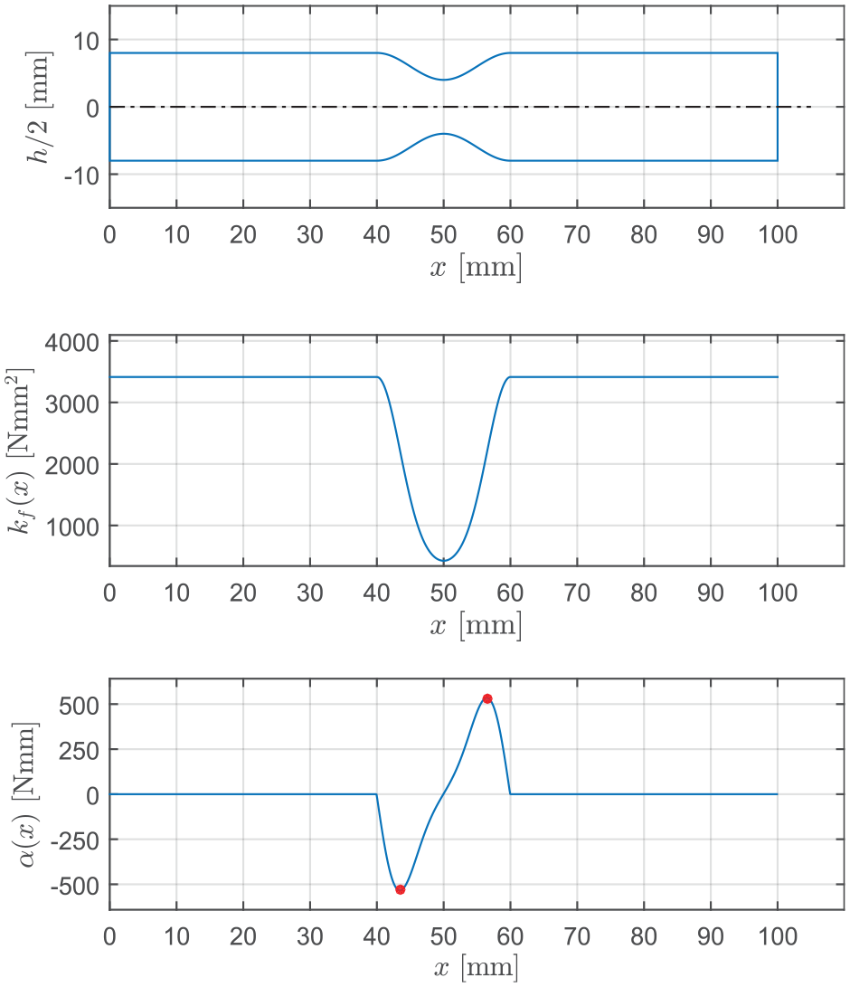
Notched body (top) with
The values of
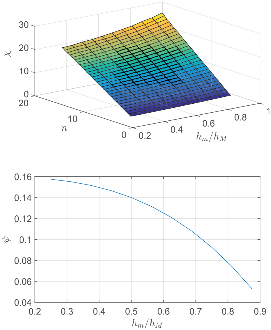
Real part of the SDI versus
We observe that
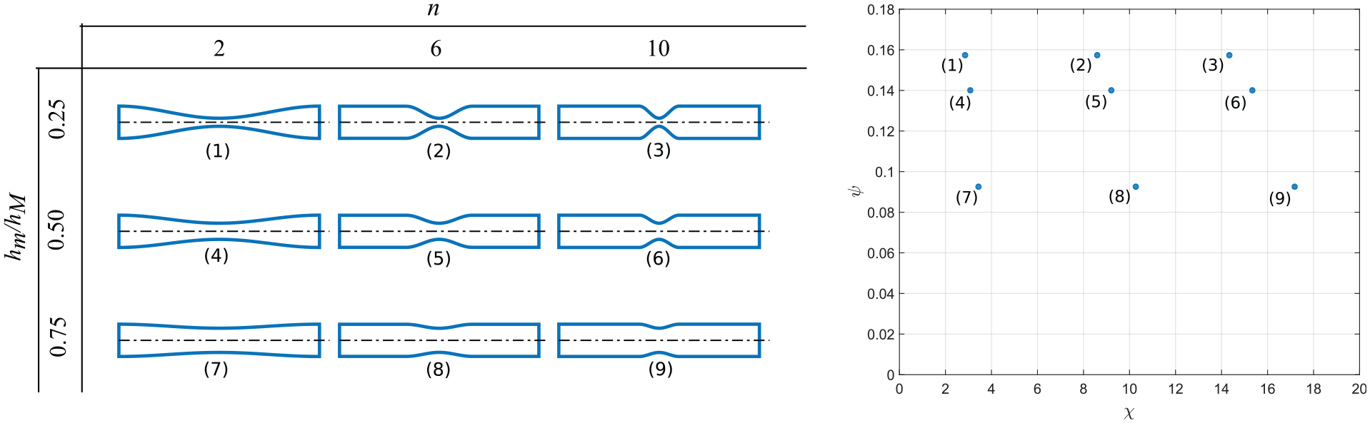
The SDI is computed for nine bodies whose notches are determined by different
5.2. Modeling
We study the deformation of this class of bodies owing to a constant external moment
For the motivations reported in Section 4.1, we assume that the finite element technique provides the most accurate estimation of the deformation, among all the techniques; therefore, the results will be presented in terms of error with respect to those obtained by FEA. The aim of the work reported in this section is to assess whether it is possible to identify a particularly convenient modeling technique depending on the distribution of the softness in the notched body. We have analyzed a total of 21 bodies which differ in
The reader should keep in mind that the investigation carried out here is limited to linear elastic material. Moreover, unlike FEM, the other methods do not account for shear effects or warping of the cross-section. Further discussion on these aspects is postponed to Section 8.
5.2.1. FEA
FEA is performed by means of the commercial software ABAQUS Standard®. In all the cases considered, the body is discretized in 5,712 hexahedral elements with reduced integration, for a total of 27,151 nodes. The kind of element selected has 20 nodes. We have selected hexahedral elements instead of tetrahedral, because in this case they allow for the creation of a structured mesh. By properly setting the element size, a subset of nodes can be located at the neutral plane of the body. This is necessary to extract results in terms of nodal displacements that can be compared with those obtained by the other modeling techniques adopted in this work, which are all relative to the neutral plane. All the simulations account for large deflections and have been performed using an iterative solver. The end moment load is gradually applied as a linear function of pseudo-time, in 100 steps. The material is considered linear elastic, with Young’s modulus
The results for each simulation are then exported and imported into the MATLAB® environment, in which the displacements of the nodes on the neutral plane are extracted and plotted, to be compared with the results obtained with the other modeling techniques.
5.2.2. NMSA
The structure is discretized into 6 beam elements having equal length
5.2.3. EA
We study the deformation of a cantilever beam with variable cross section subject to end moment load
and the boundary conditions are as follows:
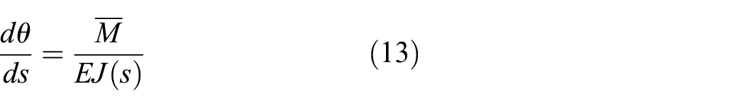
We compute the deformed configuration of the beam by numerical integration of Equation (13) performed in MATLAB® using the built-in function
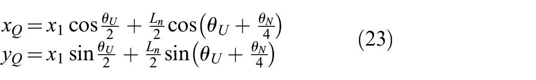
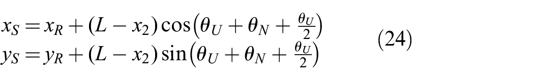
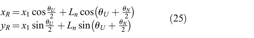
The Cartesian coordinates of the cross section
5.2.4. LPs
The LPM uses the minimum number of parameters among the four considered techniques. In this work, we model the deformation of the notched body by means of the set of parameters defined as follows.
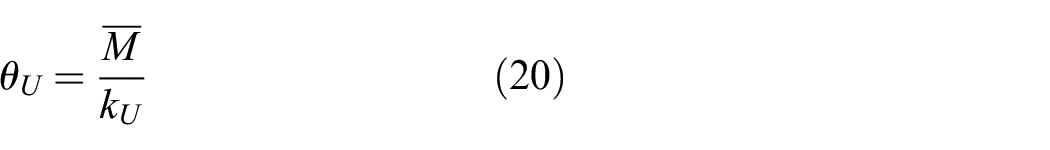
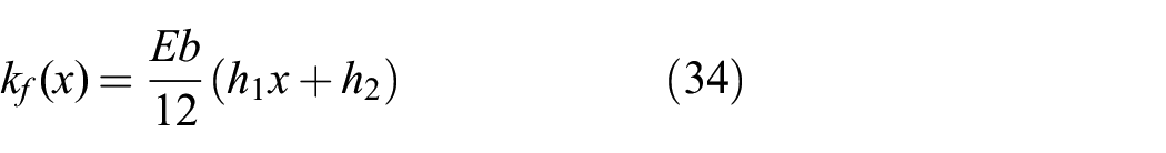
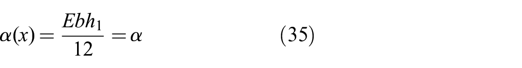
Let us denote by
where it is
The quantity

being

The multiplying factor 0.267 has been determined by imposing that a notch with
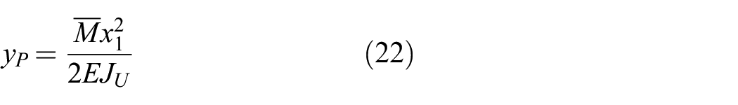
The stiffness coefficients defined previously are used to compute the coordinates of points
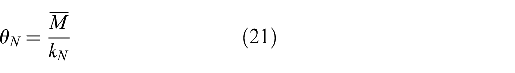
are the relative rotations between sections at points
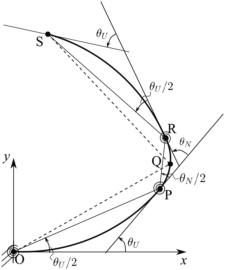
The beam is represented in two segments, denoted by the dashed broken line; the coordinates of point
As the vertical deflection of point
the slope of the line passing through
being
5.3. Results
The results obtained by using the four techniques are here reported and compared for the 21 bodies analyzed. Figure 10 shows the deformed configuration for the body with
View on the
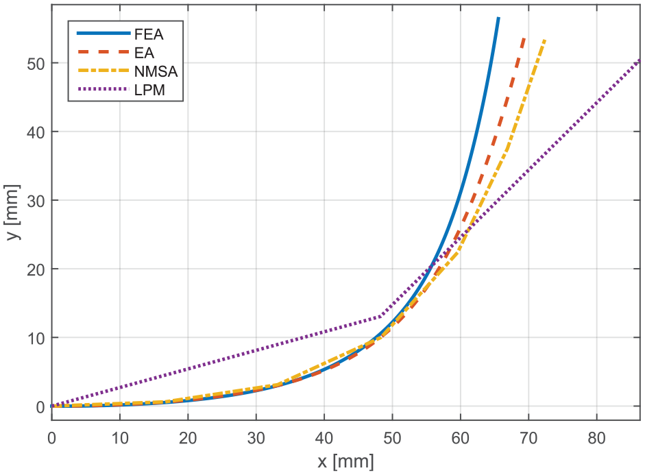
Results obtained by the four techniques for the body with
It is evident from the plot that, for the considered body, all the techniques provide results that deviate from those given by FEA; however, the error in the position

where
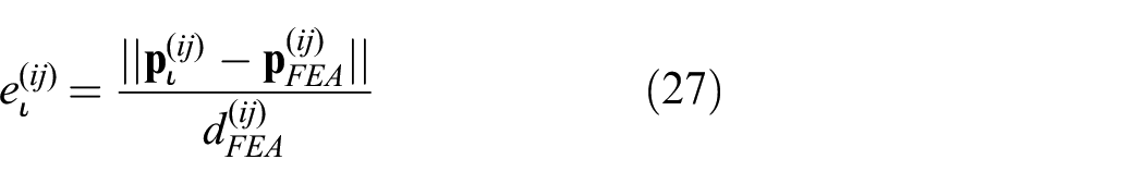
and
The plots in Figure 12 show the errors relative to bodies with different
Error

Rectangular region of
We observe that the SDI, as defined in Section 3, effectively allows to identify regions of the complex plane that correspond to a modeling technique. In Figure 13, the full colored region indicates that the denoted technique has provided an error smaller than 10%; the other regions are relative to an error up to 20%. We also note that in some cases two techniques overlap. FEA can provide highly accurate results for any body, with the proper settings; hence, we can consider that it covers the entire space represented in the plot, and it is not displayed to make the figure more readable.
The LPM as implemented in this work has been developed to model hinge-like notched bodies: the lowest
It is indeed worth keeping in mind that the plot in Figure 13 is valid for the considered techniques in the way we have employed them, and that different implementations (e.g., an alternative set of LPs) would have provided different results. Another important aspect is related to the ratio between the amplitude of the displacement and the length of the body. The higher the ratio, the higher the error for any of the techniques that we have used in this article (later, we provide the reader with some insight concerning this aspect). However, the results that we have obtained are meaningful for two reasons: on the one hand, they show that the SDI can serve as a tool to relate a body to a technique; on the other hand, they provide at least a general guideline for the choice of a modeling technique. It must be clear that the SDI, at least at this stage of the work, does not provide directions about the appropriate modeling assumptions. Any technique, however accurate, leads to poor results if used under incorrect assumptions or without carefully checking the setup. This important matter is more widely addressed in Section 8.
5.4. A further investigation on notched bodies
So far, we have compared the results obtained by four techniques on bodies characterized by Equation (19). The definition of the SDI is based on the flexural stiffness, and therefore should have general validity. However, we repeat the study on bodies having a different profile. The aim is to assess to which extent the results in Figure 13 are valid in a case which differs from the one of cosinusoidal notch.
Therefore, here we consider bodies with rectangular cross section having height which varies according to the following expression:
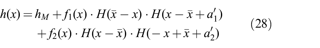
in which
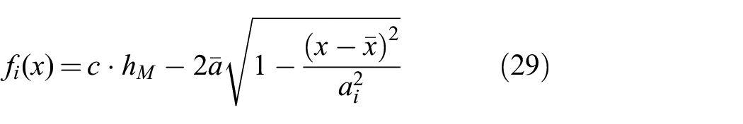
for
Figure 14 clarifies the meaning of the coefficients appearing in the expressions above.
Body with elliptical notch. The notch is obtained from two different ellipses, sharing the semiaxis
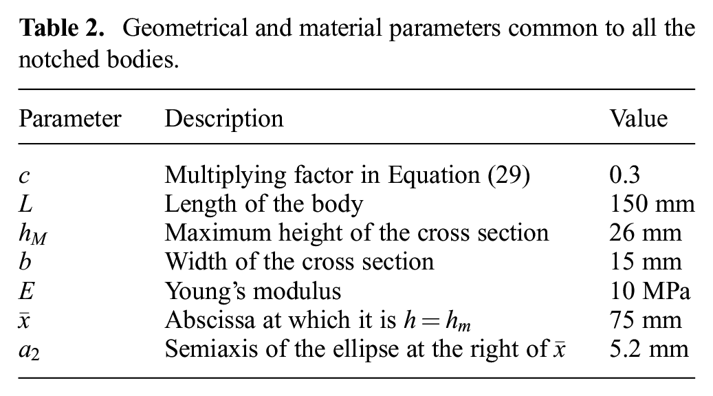
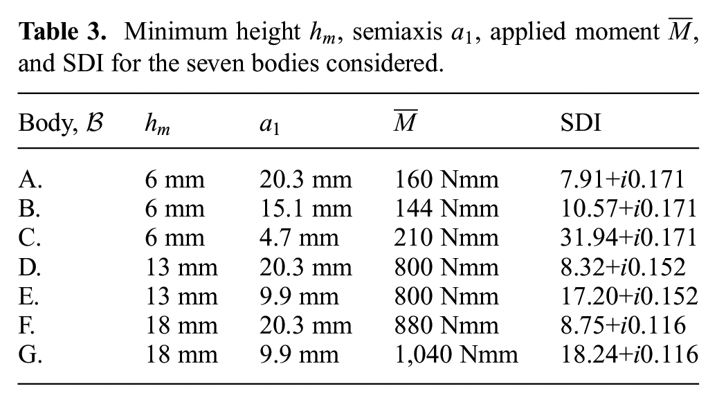
We report here the results concerning seven bodies that in our opinion are particularly meaningful. All the bodies considered are characterized by the numerical values listed in Table 2, while they differ for those in Table 3, where each body is denoted by a different capital letter.
Geometrical and material parameters common to all the notched bodies.
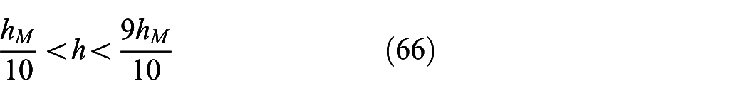
Minimum height
The four techniques are implemented as described for the previous set of bodies. The only difference consists of the numerical coefficient that appears in Equation (19): instead of 0.267, we use here 0.2. This choice is discussed at the end of this section.
Table 4 summarizes the results of this investigation. First, let us focus on EA: based on Figure 13, for bodies
Error
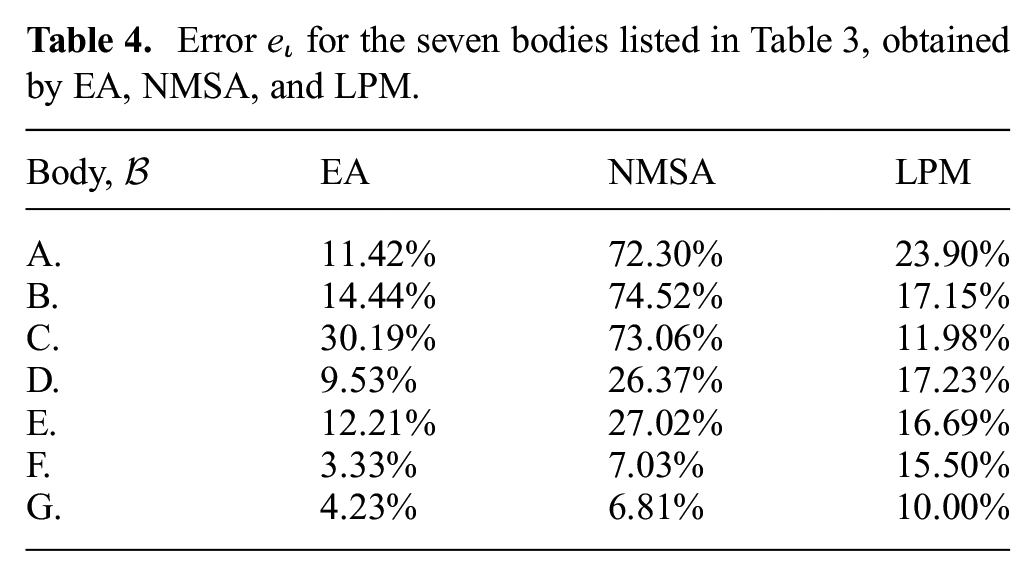
Proceeding with the analysis, we see that also results obtained by NMSA are in accordance with Figure 13: there is no need for detailed comments about this set of results. In contrast, the case of LPM merits great attention. As we stated in Section 5.3, the boundaries of the regions of the complex plane that we can draw for a LPM strongly depend on the specific set of LPs that we define and use. It is true that LPM comes at relatively low computational cost; however, its drawback is that it is not always easy to assign the value of the parameters. In particular, in cases such as those investigated in this article, in which the flexural stiffness is not constant along the axis of the bodies, the identification of the equivalent length in Equation (18) may be tricky. A small difference in a coefficient, such as the numerical value in Equation (19), can relevantly increase or decrease the accuracy. To give a flavour of this fact, we point out that using the coefficient 0.25 instead of 0.20, allows the error
6. SDI for particular cases
The results found so far suggest that the SDI may allow bodies to be classified based on the distribution of the structural properties. However, further considerations must be made to prove its general validity: only the region of the complex plane shown in Figure (13) has been explored so far. In this section, we fill this gap by considering structures that turn out to be particularly meaningful for the purpose of this work. First, we discuss the case of bodies made of multiple materials; then, we introduce classes of bodies for which
6.1. Body made of multiple materials
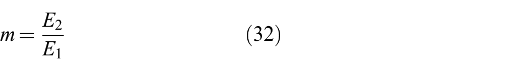
Let us consider a body made of two materials having different Young’s modulus:
that is used as a multiplying factor to transform the area of the cross section in the direction parallel to the neutral axis: in other words, the width of the region with
6.2. Bodies with
A subset of bodies is characterized by

being
and, therefore,
Under this condition, the first factor in the definition of
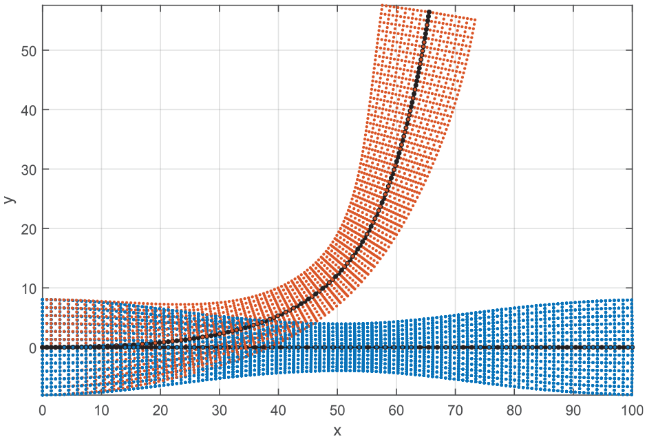
6.3. Soft continuum arm with uniform cross section
Let us consider a continuum arm,
Figure 15 shows the arm, initially straight, in the deformed configuration as computed by FEA, in comparison with the deformation obtained by applying EA and NMSA. In this case, EA provides results that slightly differ from those computed by FEA: it is, in fact,
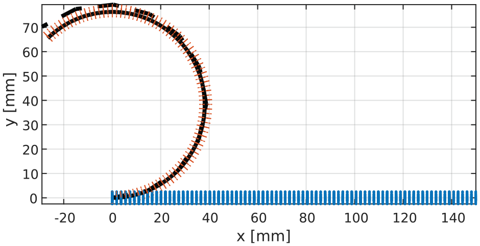
Continuum arm subject to end moment load. The blue and red dots represent the nodes in FEA in the undeformed and the deformed configuration, respectively. The solid black line denotes the solution computed by EA and the dashed black line the solution obtained by NMSA.
For this class of bodies,
6.4. Bodies with
Here, we consider the classes of bodies characterized by
where
The first derivative of the stiffness is
We observe that
is positive everywhere. Hence, it is
for
for
In both cases,
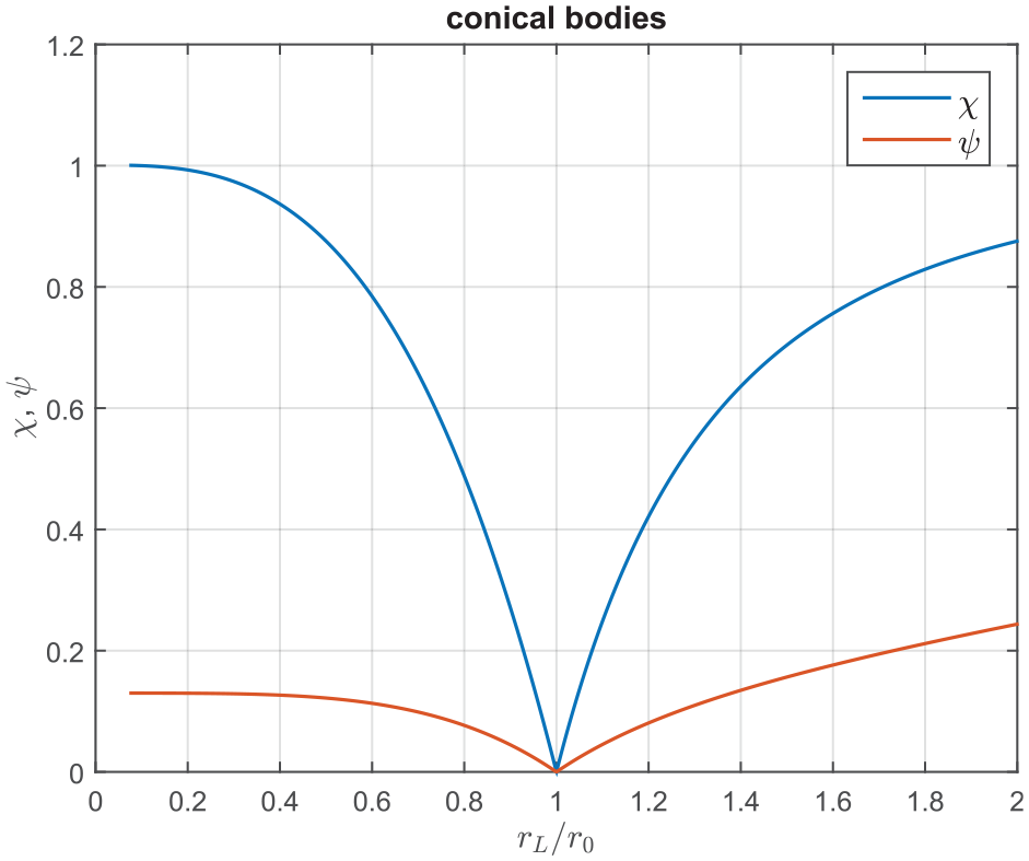
Plots of
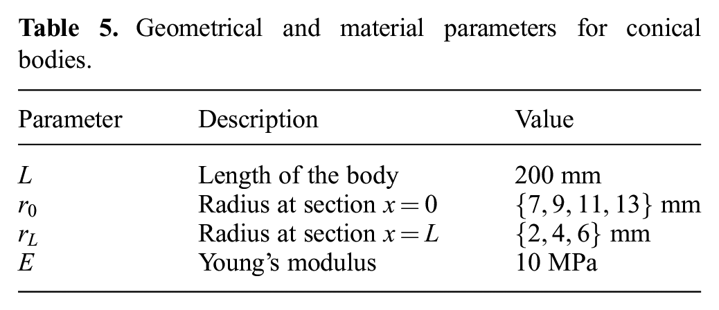
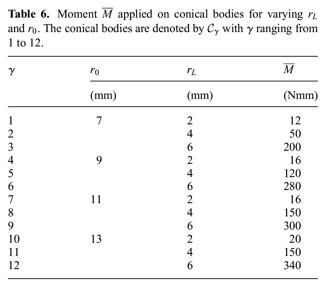
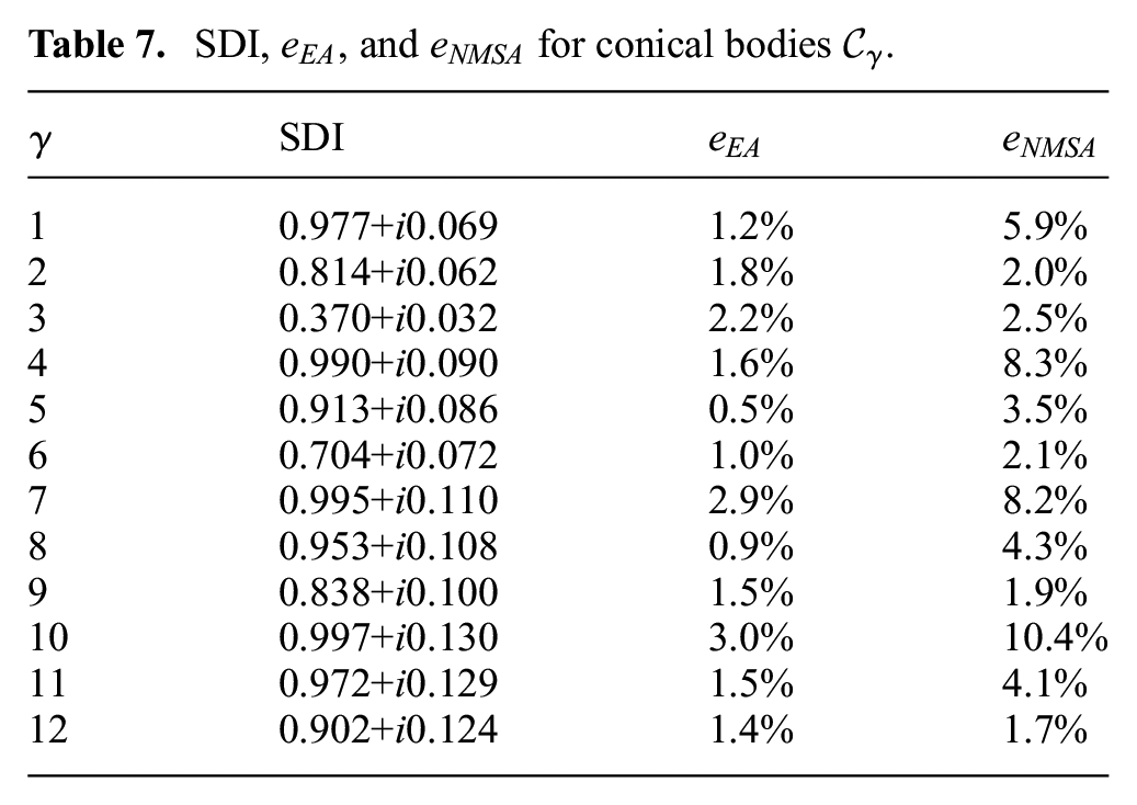
It is fairly intuitive that for this class of bodies, the most suitable choice in terms of modeling technique is represented either by EA or NMSA. According to Figure 13, by using EA we should compute the position of the free end section with an error up to 10%. To verify that this is true, we have used the techniques on 12 conical bodies. Material and geometrical parameters for this study are listed in Table 5, whereas the applied external moment at the free end section is reported in Table 6.
Geometrical and material parameters for conical bodies.
Moment
Both techniques perform as expected. Figure 17 allows a comparison of the results given by EA, NMSA, and FEA for body
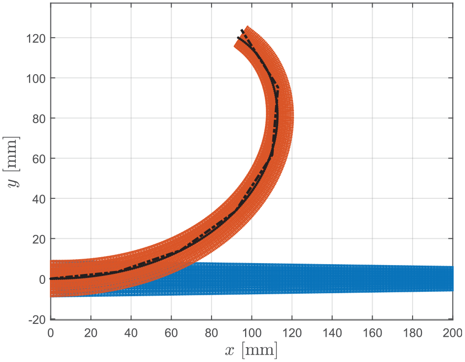
Deformation of a conical body having
SDI,
Conical bodies are not the only ones for which is it

with
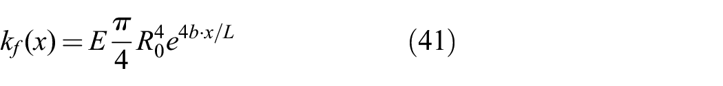
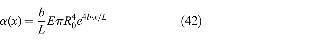
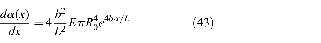
As we observed for conical bodies, from Equation (43) we infer that
for
for
We reach the same conclusions drawn for conical bodies. In addition, we can note that the case
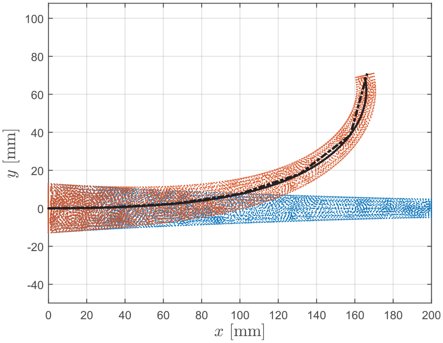
Results obtained by FEA, EA (solid line), and NMSA (dashed line) for a body with circular cross section the radius of which decreases exponentially along the length.
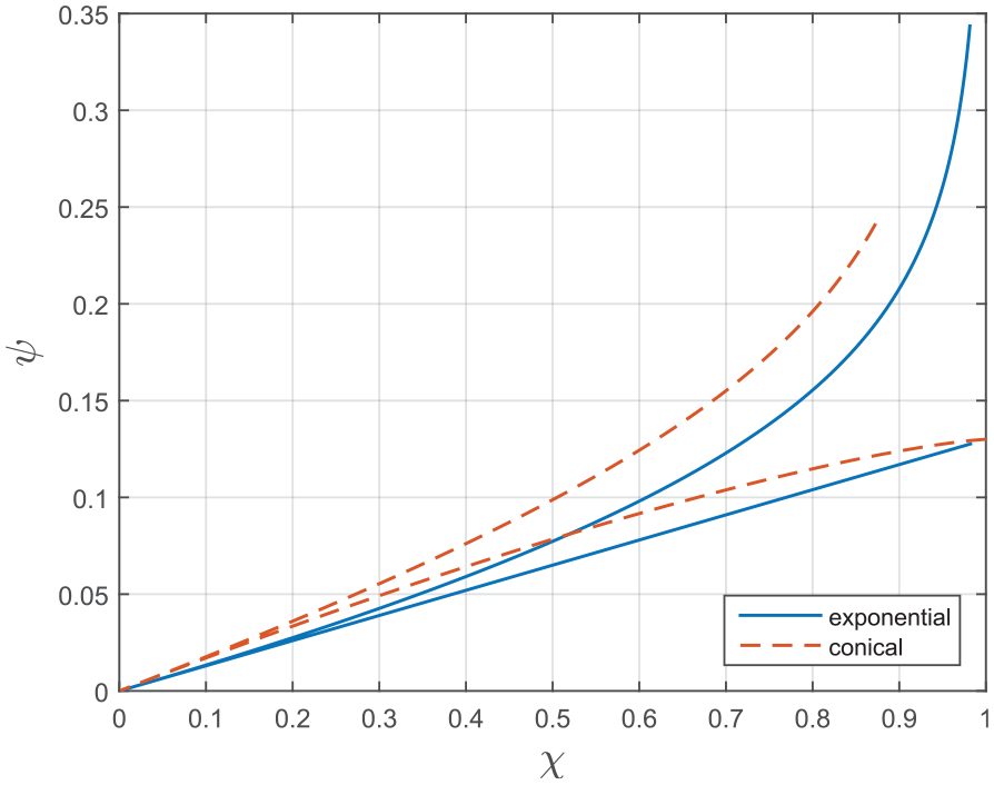
SDI for bodies with exponential profile (solid blue line) and conical bodies (dashed red line). Numerical values of material and geometrical parameters for which the curves are computed are reported in the text.
6.5. Bodies with
Finally, we provide an example of a class of bodies for which it is
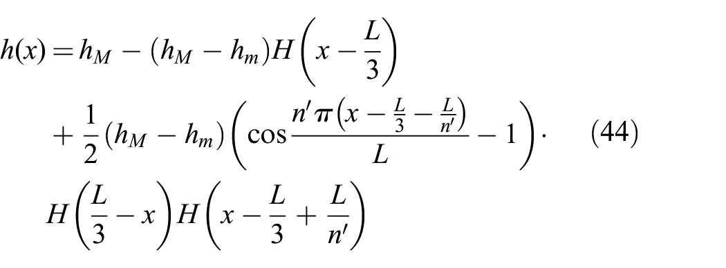
Again,
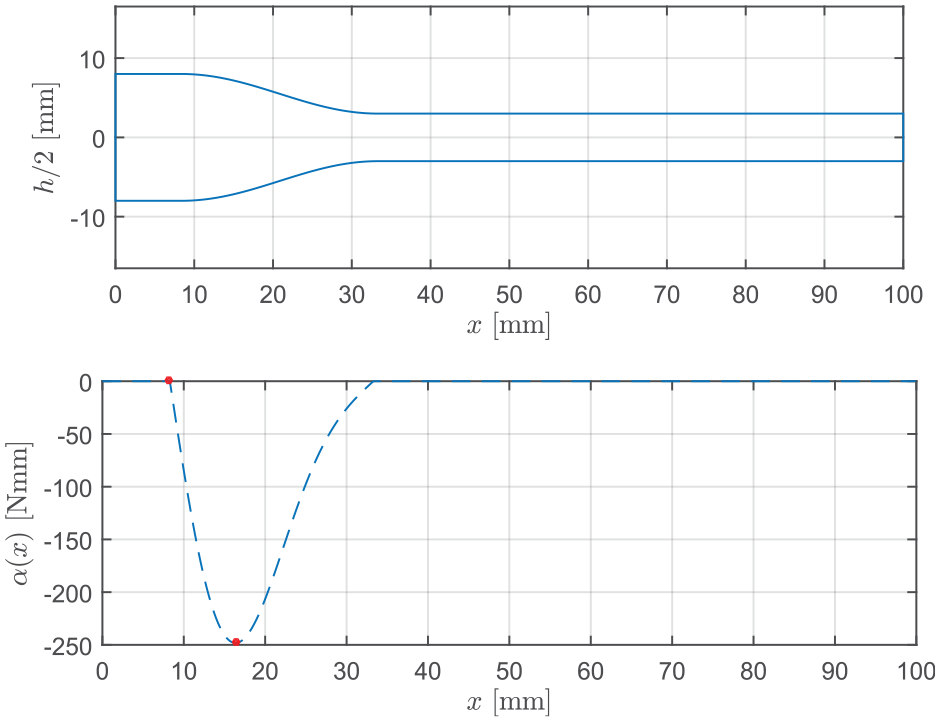
Body with variable cross section (top), characterized by the negative real part of the SDI. The first derivative of the flexural stiffness is plotted (bottom) and the minimum and the closest maximum are highlighted by red dots.
In this case,
Body with decreasing height of the cross section (top) similar to the body in the previous figure but with different ratio
7. SDI for optimization
So far, we have observed that the SDI can lead to a consistent partition of the complex plane, allowing us to draw regions that we can link to one or more modeling techniques. This encouraging result pushes us to investigate another aspect: can the SDI be useful for design purposes? Can it play a role in the structural optimization of a soft link?
In this section, we present an optimization problem that has helped us to better assess the validity and the usefulness of the SDI. Thanks to its simplicity, the example reported here shows how the SDI can guide us in the optimization.
7.1. Statement of the problem
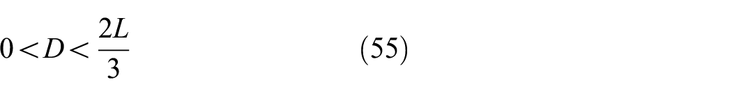
Let us design a link of length
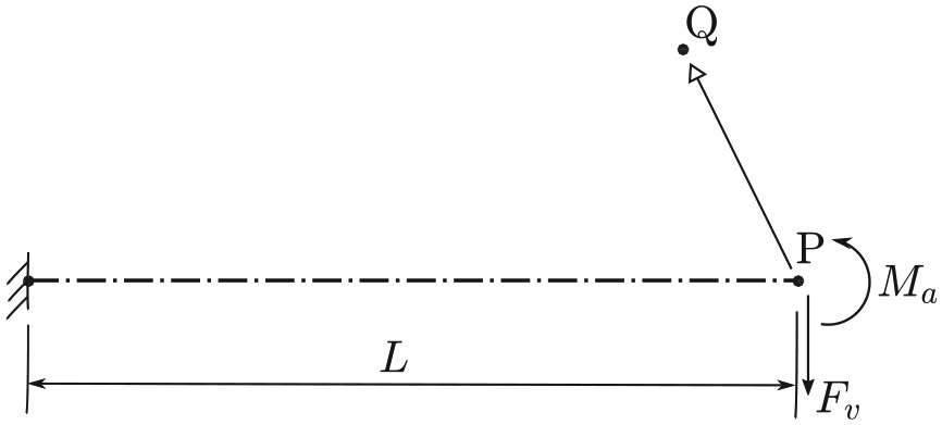
The body is clamped at the origin of the system of coordinates and its free end
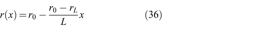
To work with a low number of design variables and simplify the discussion, we assume that the body is made of a single material that we treat as linear elastic. In addition, we prescribe that the body has circular cross section whose diameter can range between a minimum
7.2. Optimization
A very simple and intuitive model for this problem is represented in Figure 23: the body consists of two quasi-rigid links connected by a thin, circular beam that behaves as a flexural pivot and geometry of which has to be found. The compliance of the body can be considered concentrated between points

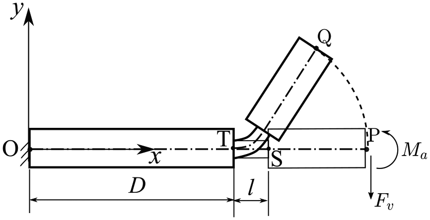
The body, initially straight, deforms under the applied moment
The two rigid links have given diameter
Unlike the body in Section 5.2.4, here the beam is subject to a non-constant moment, owing to the force
with
The displacement of

The objective of the optimization is to minimize the distance between point

Here, we perform optimization in MATLAB environment by the
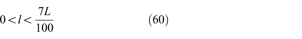
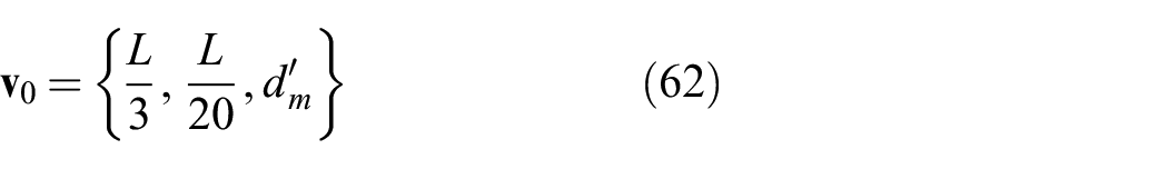
Moreover, the solution is searched accounting for the following set of constraints:


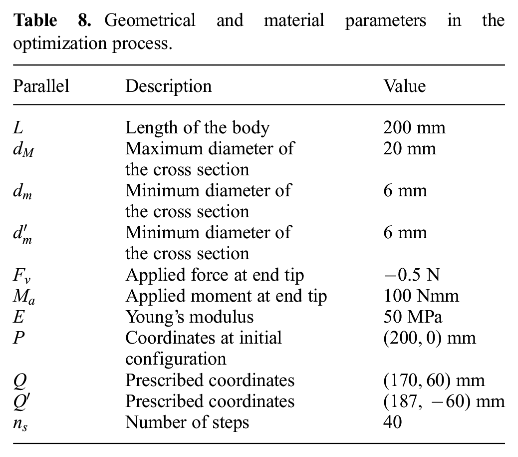
If we adopt the numerical values listed in Table 8, we find that the solution is
Geometrical and material parameters in the optimization process.
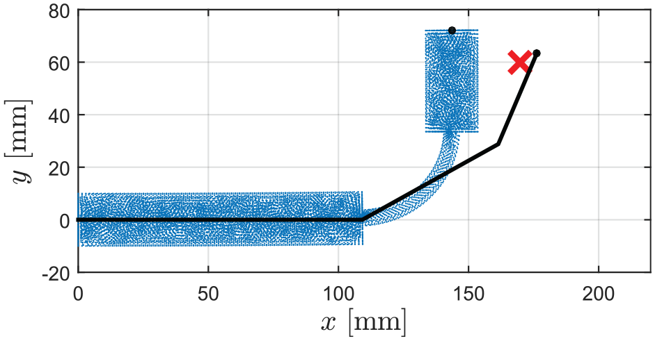
Deformation of body
As the problem seems to require a larger computational effort, let us try again using a different technique, setting the optimization problem by using NMSA. The objective function has still the form in Equation (49), but now it depends on a different set of design variables:

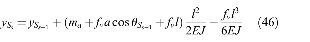
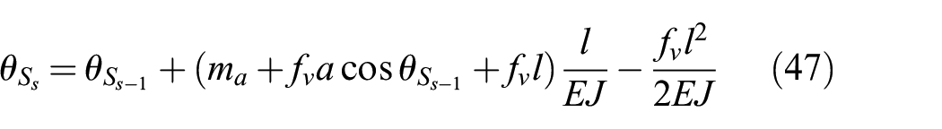
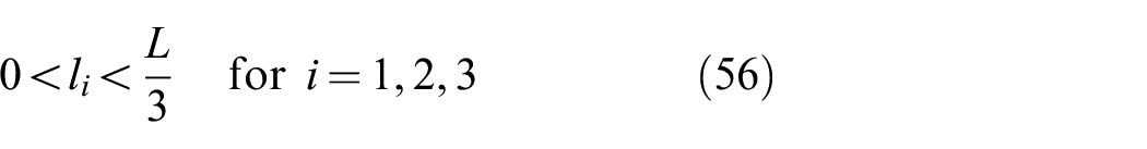
whose meaning is clarified by Figure 25, which also shows the global enumeration of the nodes of the discretization. The structure is divided into five elements, serially connected; the nodes are enumerated from 1 to 6, being the first node clamped. As was done for the notched body, the load is applied incrementally in
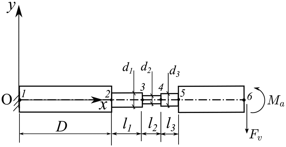
Schematic representation of the model based on NMSA. Nodes are numbered from 1 (clamped) to 6 (on which the loads are applied). The diameter and the length of elements between nodes 2 and 5 are treated as design variables, together with the distance
The optimization is performed under the following constraints:

and from an initial guess based on the solution computed by LPM:
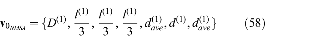
where
Deformation of body
Based on the results reported previously, we might conclude that the LPM is not suitable at all, and that we should have recurred to NMSA from the beginning, possibly with a number of elements greater than five, to further reduce the error. However, this would be a mistake. We prove this with a simple example. Let us consider a similar problem, with a different prescribed point


and starting the search from the initial guess
we find that the objective function takes the value
Deformation of body
It is evident that, in the last case, the LPM represents a good candidate for the optimization process. Compared with NMSA, it is easier to implement and requires familiarity with the classical beam theory only. In addition, it makes the optimization process notably faster than that involving NMSA, owing to the lower number of design variables. In fact, the price that we pay for a more accurate model is related to the computational cost: to find the geometry of
These results show that the suitability of the modeling technique should be evaluated for each specific case. Can the SDI help us to assess whether we have chosen an appropriate technique, without verifying the results by FEA or other computationally expensive methods?
7.3. The role of SDI in optimization
We now recapitulate all the results found in the previous section, and we compare the bodies
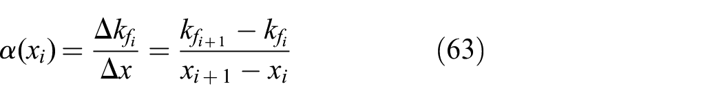
Figure 28 shows the profile of the three bodies and the function
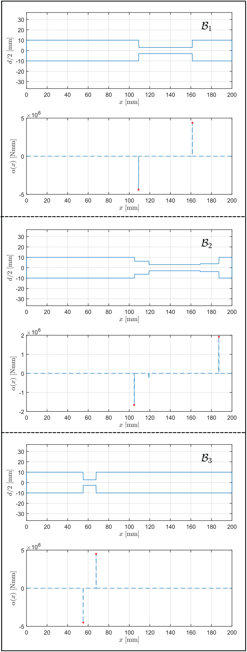
Profiles of the bodies
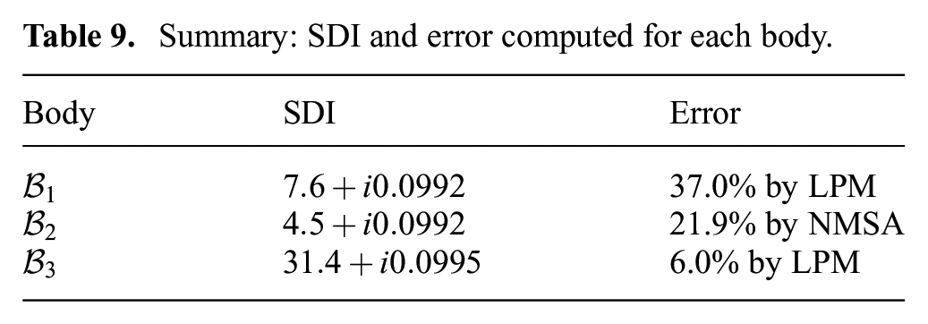
Summary: SDI and error computed for each body.
Concerning the latter, we provide in the following a further example of optimization, based on a different approach. The aim is to show that it is possible to choose a modeling technique a priori and use it for a constrained optimization whose constraints are written based on the SDI.
7.4. Optimization constraints based on SDI
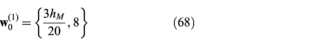
Let us return again to the geometry used in Section 5. This time, the objective is to design a notched body that undergoes the vertical displacement
In this optimization problem, we treat the parameters

Numerical values of all other parameters are assigned as reported in Table 1 and we adopt the same system of coordinates used so far. We choose to implement the model using the EA, with the same settings described in Section 5.2.3; the applied moment is

and we perform the optimization imposing the following constraints:

starting the search from
The solver succeeds to find a local minimum while satisfying the assigned constraints: at the point
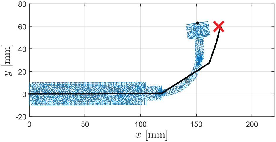
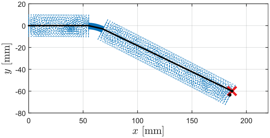
However, we see from Figure 29a that there is a discrepancy between results obtained by EA and by FEA: the coordinates of the end point of the neutral axis of the body are
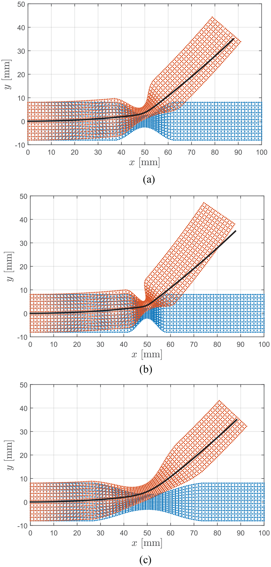
Comparison between FEA and EA for the three bodies obtained by optimization: (a)
We find that the value of the objective function for
From what has been reported above, we draw two conclusions: (i) as expected, the problem admits more than one solution, i.e., there is more than one body fulfilling the prescribed requirement; and (ii) solutions may largely differ in terms of error

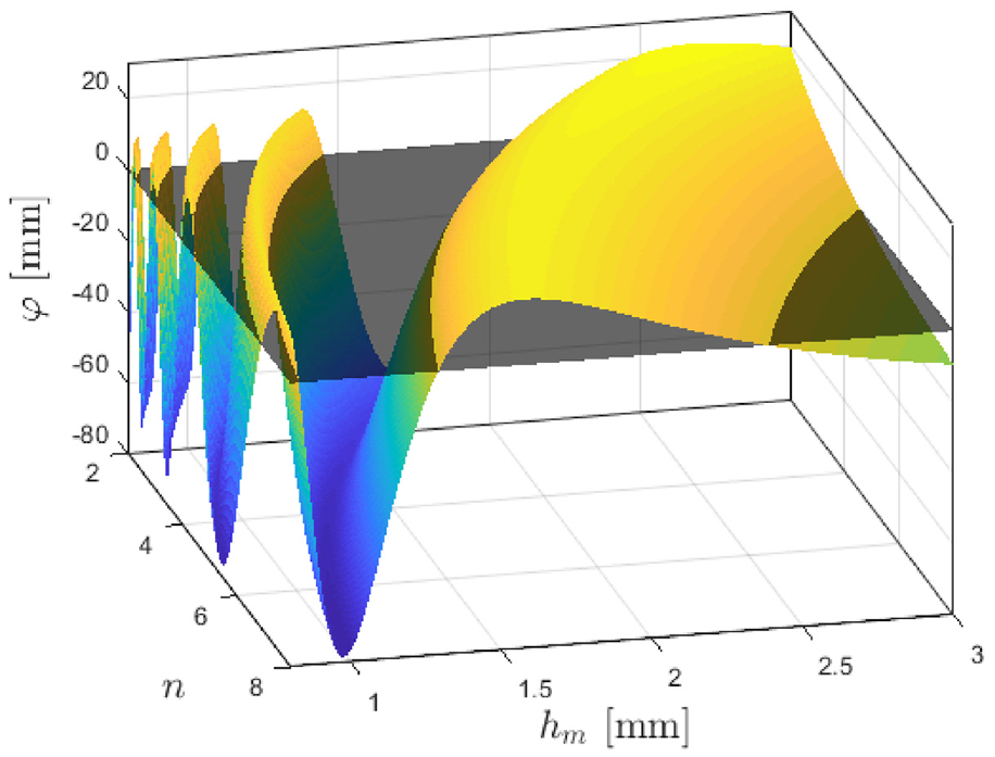
Function in Equation (65). The plot is found by means of implementation of EA as described in Section 5. The black transparent patch denotes the plane
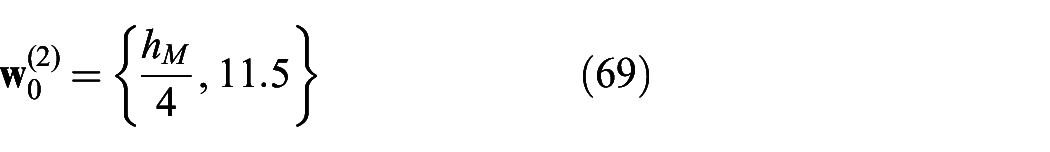
and we perform again the optimization starting the search from
It is also worth pointing out that the bodies in Figure 29a and (b) have SDI equal to
8. Discussion
As stated in Section 2, the choice of a convenient modeling technique is crucial not only when analysis must be performed, but especially when it must be used for synthesis. For analysis, the choice depends of course on the specific phenomenon or condition that has to be modeled. For instance, finite elements are powerful when the mechanical stress and strain must be computed, or when contact between bodies (or even self-contact within the same body) occurs. However, if the objective of the analysis is the computation of the deformed configuration under an external load, or the preliminary design of a soft body, finite elements are not necessarily needed. We have shown that accurate results can be obtained, in some cases, by using alternative techniques, at a much lower computational cost and in a way at the reach of our intuition. In the case of synthesis, we believe that the choice of a technique has a non-negligible influence on our understanding of the working principles of soft robots and, in general, of all the systems. Not without reason, in fact, several soft robots and actuators have been built based on the researchers’ intuitions and qualitative considerations: in our opinion, this is a consequence of the lack of adequate modeling approaches.
The SDI proposed in this article allows to classify bodies based on the distribution of their structural properties. To summarize, it helps in the choice of a modeling technique based on such distribution; it can be considered as a tool to gain a hint on the number of parameters and on the technique needed to model the softness of a robotic link with a given accuracy. Let us consider a body such as that described in Section 5, with the same length but with two equal notches. The SDI would be equal to that computed with the same body with a single notch: this means that the SDI suggests the same technique for both the bodies. In fact, if the body with the single notch can be effectively modeled by LPM, then the body two notches also can: the difference is that an additional LP is needed in the model. If we consider, instead, a long continuum arm with uniform cross section except for the presence of a narrow notch, the real part of the SDI would assume a great value (depending on the length of the arm) and the imaginary part would be small. This is consistent with the plot in Figure 13: the arm should be modeled by EA or NMSA. Possibly, a hybrid technique including also a LP to model the notch could be adopted.
The SDI introduced in this article accounts for the distribution of the flexural stiffness. However, this is not the only important quantity to consider. Soft bodies for robotic applications may be, in general, intended not only to bend, but also to stretch, to undergo torsion, inflation, under combination of loads that act simultaneously (point forces, distributed loads, and moments). It will be necessary to define additional indices to fully classify soft-bodied robots and develop a comprehensive set of tools to be used for analysis and synthesis purposes. The path ahead is still long.
Another important aspect concerns the assumptions on which a given modeling technique is based. In this article, for instance, we have neglected the shear effects when implementing LPM, EA, and NMSA; however, in some cases it is needed to introduce shear correction factors that depend on the geometry of the body (as explained by Timoshenko beam theory). Another assumption, widely employed in soft robotics, is that segments of the body bend with constant curvature; in some works, researchers have shown that this assumption has led to acceptable results, but this does not mean that the assumption could always be adopted. In some works, it is assumed that the cross-section does not change with the deformation (see, e.g., Renda et al., 2017: in which the area and the moment of inertia of the cross section are constant). However, warping of the section, local deformations and high local strains may play a big role. In Section 7.3, we have seen that for body
To summarize, the assumptions on which a model can be based are numerous. A further aim of our future work will be to identify criteria that encourage or discourage the use of the commonly used assumptions, based on the distribution of the structural properties of the system. To reach this goal, the first derivative of
9. Conclusions
The main objective of this work has been to highlight the importance of the distribution of the structural properties in a body undergoing large deformation and that such distribution is related to the choice of a modeling technique. We have proposed a novel index, called SDI, that accounts for the structural properties of a body performing bending.
In order to carry out a quantitative investigation, we have modeled the bending of soft bodies recurring to different techniques and we have shown that it is possible to map bodies to the complex plane using the SDI. The complex plane has been divided into regions, each corresponding to one or more modeling techniques suitable for the body under investigation, showing that the provided definition of the SDI makes a classification possible.
The achievement of a unified framework for the modeling of soft robots will require further work from the soft robotics community. We believe that this framework should include all the modeling techniques employed so far by the researchers, possibly developing hybrid techniques that could combine the use of FE, MSA, Cosserat rod theory, elastica theory, LPs, and different assumptions (for instance, the piecewise constant curvature, frequently recalled in the literature), to be selected based on the SDI of the body. We do not claim that the proposed SDI represents a fully developed and tested tool to solve the problem completely; in contrast, we believe that additional efforts are required from the soft robotics community to achieve a complete classification of soft bodies based on the distribution of their properties, and the corresponding choice of a modeling approach. We believe that other indices should be defined to account for other typical deformation modes of soft robots (for instance, tension and compression, squeezing). In this article, we have provided evidence that it is possible to find a relation between bodies and modeling techniques by means of a mathematical tool.
Footnotes
Appendix A: Invariance of SDI under inversion of x -axis
Let us consider the function
By definition, the first derivative of
Let
that is, the function
Therefore, the difference quotient
is negative. Computing the limit for
If
that is, the function
As it holds
according to the definition of
The condition above is satisfied. In fact, it is
and
It follows that
Appendix B: NMSA
Same as for the FEM, the order in which the DOFs are listed is arbitrary. In our work, following the common practise, we define the vector of nodal displacements of the
In this work, the nodal rotations
Coherently, the local stiffness matrix
in which
The local nodal displacements are expressed in the global system of coordinates by means of the transformation
where
in which it is
being
The strain energy for the
using the local quantities, or as
as a function of the nodal displacements and the stiffness matrix expressed in global coordinates. As the strain energy is invariant under coordinate transformation, it must be
from which follows that
by substitution of Equation (83).
The stiffness matrix derived so far belongs to
where
and the full stiffness matrix in global coordinates is then computed as the sum of all the extended matrices:
Similarly, all the nodal displacements in global coordinates are collected in a vector
where the subscripts f and c refer to free and constrained DOFs, respectively; the vector
which is the very well-known Hooke’s law. In order to account for large displacements, several approaches can be adopted (see McGuire and Gallagher, 1979); here, we apply the external load in a finite number of steps
where the stiffness matrix
In the initial configuration of the bodies considered in Sections 5.2.2 and 6.3, the orientation of the
and the orientation of the
being, in the global enumeration adopted,
(for a matter of convenience, the subscript f has been dropped in the expression above).
Acknowledgements
We are sincerely grateful to the three anonymous reviewers for their helpful comments and suggestions.
Funding
The author(s) disclosed receipt of the following financial support for the research, authorship, and/or publication of this article: This work was funded by GrowBot, the European Union’s Horizon 2020 Research and Innovation Programme under Grant Agreement No. 824074.