Sage Journals: Discover world-class research

Abstract

Consider deploying a team of robots in order to visit sites in a risky environment (i.e., where a robot might be lost during a traversal), subject to team-based operational constraints such as limits on team composition, traffic throughputs, and launch constraints. We formalize this problem using a graph to represent the environment, enforcing probabilistic survival constraints for each robot, and using a matroid (which generalizes linear independence to sets) to capture the team-based operational constraints. The resulting “Matroid Team Surviving Orienteers” (MTSO) problem has broad applications for robotics such as informative path planning, resource delivery, and search and rescue. We demonstrate that the objective for the MTSO problem has submodular structure, which leads us to develop two polynomial time algorithms which are guaranteed to find a solution with value within a constant factor of the optimum. The second of our algorithms is an extension of the accelerated continuous greedy algorithm, and can be applied to much broader classes of constraints while maintaining bounds on suboptimality. In addition to in-depth analysis, we demonstrate the efficiency of our approaches by applying them to a scenario where a team of robots must gather information while avoiding dangers in the Coral Triangle and characterize scaling and parameter selection using a synthetic dataset.

Keywords

Submodular optimization matroid constraints path planning multi-robot control

1. Introduction

Consider a scenario where mobile robotic sensors are used to monitor a number of regions of the ocean, each of which may require different sensing capabilities. Due to uncertain and possibly adversarial events (e.g., bad weather or piracy), there is a risk that robots may “fail” when traveling from one region to another. A fleet manager seeks a set of paths which maximizes the expected number of sites monitored while satisfying various resource constraints. For example, there may be limits imposed by the number of available robots of each type, the logistics of deploying the robots, the probability a given robot reaches its destination, or the amount of traffic a given region can support. If these constraints are “downward closed” (meaning any subset of a feasible set of paths is feasible) and satisfy an exchange property, then we can represent them using a matroid (Schrijver 2002), which generalizes linear independence to set systems and has structure amenable to optimization.

We formalize this class of exploration problems as a generalization of the orienteering problem (Golden et al. 1987), where one seeks a path which visits as many nodes in a graph as possible given a budget constraint and travel costs. In our earlier example the travel costs are the probability that a robot fails while traversing between sites, and we are looking for a set of such paths which is an independent set of a matroid, maximizes the expected number of nodes visited by at least one robot, and ensures that the probabilities each vehicle reaches its destination is above a specified threshold.

We call this problem formulation the “Matroid Team Surviving Orienteers” (MTSO) problem, illustrated in Figure 1.

Figure 1.

Illustration of an ocean monitoring scenario with various regions and sites to visit within each region marked by “X,” and the heat map indicates the risk of robot failure inferred from piracy incidents. The objective is to find a set of paths for a heterogeneous team which maximizes the expected number of sites visited subject to several constraints. Data is from the Coral Triangle Atlas (Cros et al. 2014) and the International Chamber of Commerce: Commercial Crime Services (2017).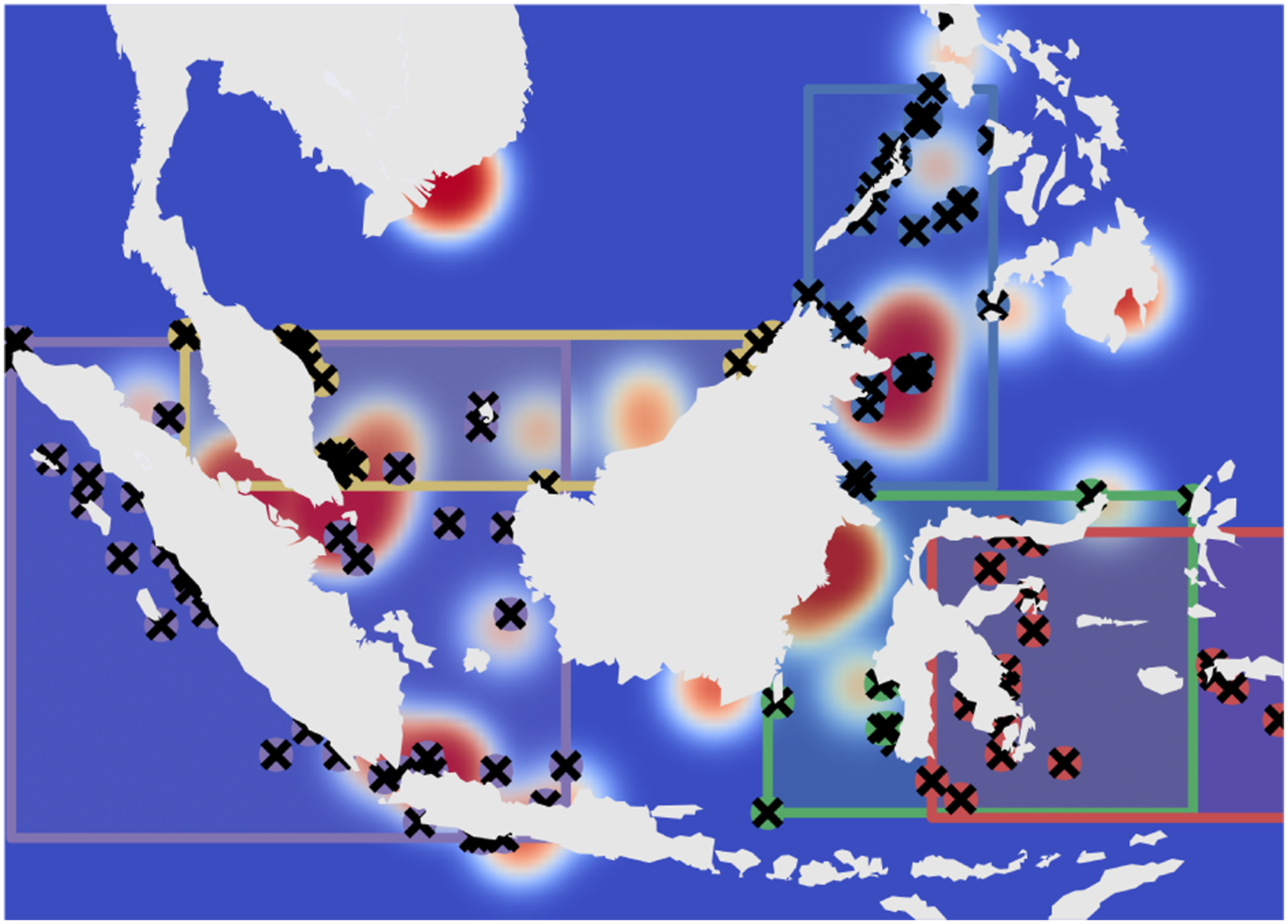

The MTSO problem is a significant generalization of our earlier work on the Team Surviving Orienteers (TSO) problem (Jorgensen et al. 2018), which only imposes a maximum team size constraint (a very special case of a matroid constraint). Both the MTSO and TSO are distinct from previous work because of the notion of risky traversal: when a robot traverses an edge, there is a probability that it fails and does not visit any other nodes. This creates a complex, path-dependent coupling between the edges chosen and the distribution of nodes visited, which precludes the application of existing approaches available for the traditional orienteering problem. The objective of this paper is to devise constant factor approximation algorithms for the MTSO problem. An efficient algorithm for the TSO was designed by exploiting a diminishing returns property known as submodularity (Jorgensen et al. 2018), which for set function f and sets A and B means that f(A ∪ B) + f(A ∩ B) ≤ f(A) + f(B). Our key technical insight is that we can further exploit submodularity of the objective function to design efficient solution algorithms for the much more general MTSO problem. We describe numerous applications of matroid constraints to path planning problems, and describe an approximate greedy algorithm which enjoys a constant factor approximation guarantee. We then develop an approach based on the accelerated continuous greedy algorithm (Badanidiyuru and Vondrák 2014) which is the state of the art for matroid optimization and provides tighter guarantees that are easily extended to more general settings. Although a number of works have considered routing problems with submodular objectives (Chekuri and Pál 2005; Campbell et al. 2011; Zhang and Vorobeychik 2016), chance constraints (Gupta et al. 2012; Varakantham and Kumar 2013), or downward closed constraints (Koç et al. 2016; Lahyani et al. 2015; Hoff et al. 2010) separately, the MTSO is novel because it combines all three aspects.

1.1. Related work

The orienteering problem (OP) has been extensively studied (Gunawan et al. 2016) and is known to be NP-hard. Over the past decade a number of constant factor approximation algorithms have been developed for special cases of the problem. The submodular orienteering problem considers finding a single path which maximizes an arbitrary submodular reward function of the nodes visited. The recursive greedy algorithm proposed in Chekuri and Pál (2005) yields a solution in quasi-polynomial time with a constant factor guarantee, and the cost-benefit greedy algorithm proposed in Zhang and Vorobeychik (2016) yields a solution in polynomial time but only has a constant factor guarantee with respect to a relaxed problem. Our work is distinct from these efforts because we consider a specific submodular function, but find a set of paths rather than a single path formed by a set of edges. The risk-sensitive orienteering problem (Varakantham and Kumar 2013) considers random edge weights and seeks to maximize the sum of rewards subject to a constraint on the probability that the path cost is large. Only a single path is considered, so there is no notion of independence between paths as in the MTSO.

A second closely related area of research is the vehicle routing problem (VRP) (Psaraftis et al. 2016), which is a family of problems focused on finding a set of paths that maximize quality of service subject to budget or time constraints. The rich vehicle routing problem (RVRP) (Lahyani et al. 2015) considers settings such as routing heterogeneous teams (Koç et al. 2016), “fleet dimensioning” (choosing team composition) (Hoff et al. 2010), and incompatability constraints (Kelareva et al. 2014). The vast majority of solution algorithms for the RVRP are heuristic (Lahyani et al. 2015) and do not consider risky traversal. A notable exception are linear temporal logical (LTL) constraints, which have exact integer programming formulations (Karaman and Frazzoli 2011) and transition system formulations (Smith et al. 2011; Ulusoy et al. 2014), the complexity of which grows exponentially in the team size. In our work, we consider a narrower yet still expressive set of constraints and derive polynomial time solution algorithms with constant factor approximation guarantees.

A third related branch of literature is the informative path planning problem (IPP), which seeks to find a set of paths for mobile robotic sensors in order to maximize the information gained about an environment. One of the earliest IPP approaches Singh et al. (2009) extends the recursive greedy algorithm of Chekuri and Pál (2005) using a spatial decomposition to generate paths for multiple robots, and provides performance guarantees using submodularity of information gain. While the structure of the IPP has many similarities to the MTSO problem (it is a multi-robot path planning problem with a submodular objective function which is non-linear and history-dependent), it captures neither the constraints nor the notion of risky traversal which are central to the MTSO problem. Our general approach is inspired by works such as Atanasov et al. (2015), which iteratively assigns paths to each robot, but for the MTSO problem we further exploit the problem structure to derive constant factor guarantees.

A handful of papers apply submodular maximization and matroid constraints directly to robotics applications. In Jawaid and Smith (2015), path constraints are represented using a p-system (which generalizes a matroid), and a submodular maximization problem with p-system constraints is solved to find the approximately most informative path for a single agent. Multi-robot task allocation problems are cast as decentralized submodular maximization problems with matroid constraints by Segui-Gasco et al. (2015) (who considers private reward functions), and Williams et al. (2017) (who considers communication constraints). In both cases the objective is to assign robots to tasks, rather than to find a high reward set of paths for a team of robots. Recent work by Corah and Michael (2019) and Robey et al. (2021) consider the distributed optimization setting for applications in informative path planning and task assignment—though neither setting considers risky traversal. The work by Segui-Gasco (2017) and Robey et al. (2021) is notable as it uses the (accelerated) continuous greedy algorithm which is the most similar to our work (despite a different application). In our work we use an orienteering problem oracle in order to find high quality paths for each robot while considering risky traversal. This requires different analysis which utilizes results on approximate greedy algorithms for submodular maximization subject to matroid (Fisher et al. 1978) and p-system (Calinescu et al. 2007) independence constraints.

Statement of Contributions: Matroids have been applied with great success to many fields of engineering such as electrical and structural network design (Murota 2009), but they have rarely been used for robotic routing problems. The contribution of this paper is six-fold. First, we propose a generalization of the TSO problem, referred to as the Matroid TSO problem. By considering matroid constraints, we extend the state of the art for the team orienteering problem, and by considering the risky traversal model we extend the state of the art for the rich vehicle routing problem. Second, we demonstrate how to use matroids to represent a variety of constraints such as coverage, deployment, team size limitations, traffic constraints, team-wise risk constraints, and nested cardinality constraints. Third, we extend the approximate greedy algorithm from Jorgensen et al. (2018) to the MTSO setting, and prove that the value of its output is at least $\frac{p_{s}}{p_{s} + λ} OPT$ , where OPT is the optimum value, p_s is the per-robot survival probability threshold (in practice, p_s is close to unity), and 1/λ ≤ 1 is the approximation factor of an oracle routine for the solution to the orienteering problem. Fourth, we extend the accelerated continuous greedy algorithm (Badanidiyuru and Vondrák 2014) to the MTSO problem, which is its first application to robotics. We develop a fast implementation specific to the MTSO and show its output is at least $(1 - δ) (1 - e^{- p_{s} / (λ + δ p_{s})})$ , where δ ≪ 1 is the discretization step size. Fifth, we demonstrate the effectiveness of both algorithms for complex problems by considering an environmental monitoring application and give an empirical timing characterization for both algorithms. Finally, we highlight a number of extensions of this work in detail, such as p-system constraints, linear packing constraints, and coverage variants.

This paper is a significant expansion of our conference paper Jorgensen et al. (2017a), which introduced the MTSO and greedy algorithm. In particular, we present and analyze the accelerated continuous greedy algorithm which is a new approach to the problem that provides stronger guarantees with broader applications. As mentioned above this requires extending the analysis from Badanidiyuru and Vondrák (2014) to apply to the case where the greedy problem can only be approximately solved and providing a novel method of evaluating the multilinear extension for the MTSO problem. We have also significantly expanded the numerical experiments and discuss extensions beyond matroids.

Organization: The rest of this paper is organized as follows. In Section 2 we review key background information necessary for our results. In Section 3 we present the formal problem statement for the MTSO and describe several applications in Section 4. In Section 5 we outline the algorithms and give performance guarantees. Section 6 demonstrates the practicality of our algorithm via numerical experiments. In Section 7 we discuss a number of extensions of our work which can be solved using the continuous greedy algorithm. Finally, in Section 8, we draw our conclusions and discuss directions for future work.

2. Background

2.1. Sets and submodular functions

Submodularity is the property of “diminishing returns” for set functions. The following definitions are summarized from Krause and Golovin (2014). Given a set $X$ , its possible subsets are represented by $2^{X}$ . For two sets X and X′, the set X′ \ X contains all elements in X′ but not X. A collection of disjoint subsets ${X_{m}}_{m = 1}^{M}$ is called a partition of $X$ if $\cup_{m = 1}^{M} X_{m} = X$ . A set function $f : 2^{X} \to R$ is said to be normalized if f(∅) = 0, and to be monotone if for every $X \subseteq X^{'} \subseteq X$ , f(X) ≤ f(X′). A set function $f : 2^{X} \to R$ is submodular if for every $X \subseteq X^{'} \subset X$ , $x \in X ∖ X^{'}$ , we have

f (X \cup {x}) - f (X) \geq f (X^{'} \cup {x}) - f (X^{'}) .

The quantity on the left hand side is the discrete derivative of f at X with respect to x, which we write as Δf(x∣X).

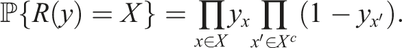
The multilinear extension of a submodular function f at $y \in {[0,1]}^{| X |}$ can be understood as taking the expected value of the function with respect to a random set R(y) which contains each item $x \in X$ with probability y_x ∈ [0, 1]. Formally, we have for $x \in X$ ,

P {x \in R (y)} = y_{x},

and for

X \subseteq X

P {R (y) = X} = \prod_{x \in X} y_{x} \prod_{x^{'} \in X^{c}} (1 - y_{x^{'}}) .

The multilinear extension of f at y is then defined as the expected value of f(R(y)):

F (y) : = E [f (R (y))] = \sum_{X \subseteq X} f (X) \prod_{x \in X} y_{x} \prod_{x^{'} \in X^{c}} (1 - y_{x^{'}}) .

For optimization problems the multilinear extension is used in a similar fashion as a linear programming relaxation of a mixed integer program, where integer variables (i.e., whether element x is in the solution) are replaced by continuous relaxations (i.e., y_x ∈ [0, 1]), and the resulting solution is rounded to get a set. We discuss this optimization framework more in Section 2.3.2.

2.2. Independence systems and matroids

The following definitions are summarized from Schrijver (2002). An independence system is a tuple of a finite ground set $X$ and a downward closed family of independent sets $I \subseteq 2^{X}$ , that is if I′ ⊆ I and $I \in I$ , then $I^{'} \in I$ . A base is an independent set $I \in I$ which is inclusion-wise maximal, that is for every $x \in X ∖ I$ , we have $I \cup x \notin I$ . A matroid $(X, I)$ is an independence system for which all bases have the same size (which is called the rank of the matroid), hence it extends the notion of linear independence to sets. There are many equivalent characterizations of matroids which are outside of the scope of this work, we refer the interested reader to Schrijver (2002) for more detail.

2.3. Approximate greedy algorithms

Given a matroid $(X, I)$ and a submodular function f, a typical submodular maximization problem entails finding a set $X \in I$ that maximizes f. In general finding an optimal solution, X*, requires an exponential number of evaluations of the function, is NP-hard for special cases such as coverage functions (Fisher et al. 1978), and cannot be approximated to closer than factor (1 − e⁻¹) in polynomial time.

2.3.1. Greedy algorithm

Given a matroid $(X, I)$ with rank K and an independent set X, the feasible set, $X_{F} (X, I)$ , is the set of all items not in X which can be added to X while preserving independence:

X_{F} (X, I) : = {x \in X ∖ X ∣ X \cup {x} \in I} .

The greedy algorithm constructs a set ${\bar{X}}_{K}$ by iteratively adding an element x from the feasible set which maximizes the discrete derivative of f at the partial set already selected. In other words, the ℓth element satisfies:

{\bar{x}}_{ℓ} \in \underset{x \in X_{F} ({\bar{X}}_{ℓ - 1}, I)}{argmax} Δ f (x ∣ {\bar{X}}_{ℓ - 1}),

and items are chosen until no more can be added, that is

X_{F} ({\bar{X}}_{K}, I) = \emptyset

. If the function f is monotone and non-negative, the greedy algorithm will choose K items, where K is the rank of the matroid

(X, I)

. We refer to the optimization problem above as “the greedy sub-problem” at step ℓ. A well-known theorem proven by Fisher et al. (1978) states that if f is a monotone, normalized, non-negative, and submodular function, then

f ({\bar{X}}_{K}) \geq 1 / 2 f (X^{*})

. This is a powerful result, but if the set

X

is large we might only be able to approximately solve the greedy sub-problem.

An α–approximate greedy algorithm constructs the set ${\hat{X}}_{K}$ by iteratively adding elements which approximately maximize the discrete derivative of f at the partial set already selected. Formally, for some fixed α ∈ (0, 1], the ℓth element ${\hat{x}}_{ℓ}$ satisfies

Δ f ({\hat{x}}_{ℓ} ∣ {\hat{X}}_{ℓ - 1}) \geq α Δ f (x ∣ {\hat{X}}_{ℓ - 1}), \forall x \in X_{F} ({\hat{X}}_{ℓ - 1}, I) .

In this setting, Calinescu et al. (2007) shows in Appendix B that the value of the approximate greedy set is close to optimal:

Theorem 1

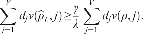
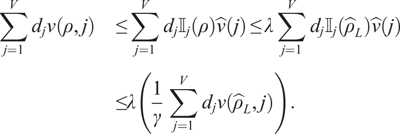
Approximate greedy guarantee Calinescu et al. (2007). Let $(X, I)$ be a matroid with rank K and $f : 2^{X} \to R^{+}$ a non-negative monotone submodular set function. If ${\hat{X}}_{K}$ is a set chosen by an α-approximate greedy algorithm, then

f ({\hat{X}}_{K}) \geq \frac{α}{α + 1} f (X), for all X \in I .

Note that while the approximate greedy algorithm is simple and relatively fast, in the best case (α = 1) the guarantee is 1/2, but the state of the art has a 1 − e⁻¹ ≃ 0.63 guarantee with matching hardness bounds.

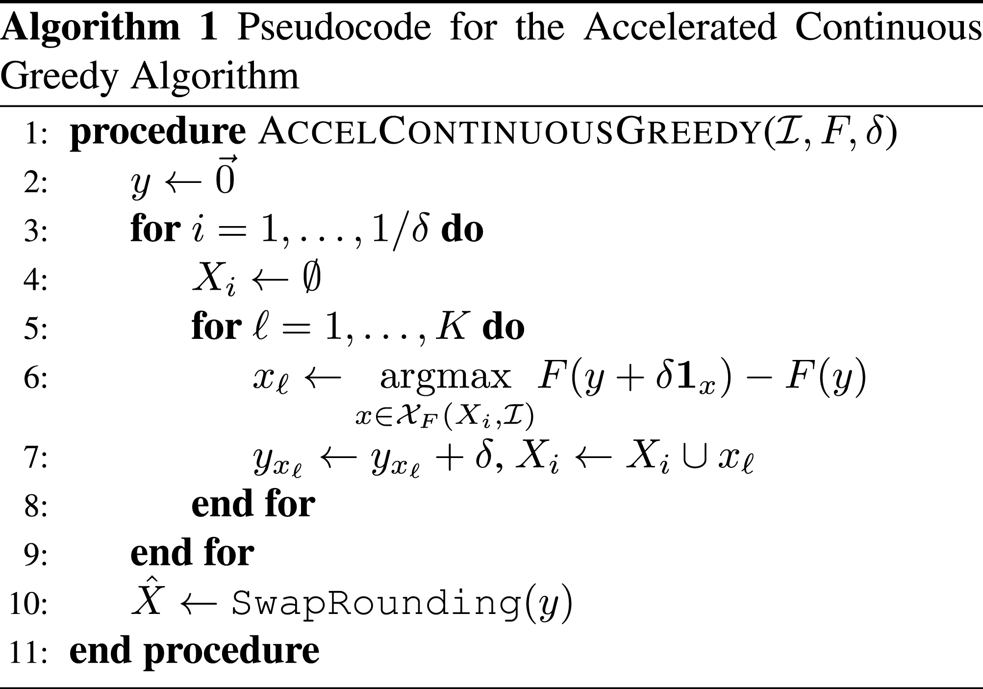
2.3.2. Accelerated continuous greedy algorithm

The accelerated continuous greedy algorithm (ACGA) recently proposed by Badanidiyuru and Vondrák (2014) optimizes the multilinear extension using coordinate gradient ascent (see pseudocode in Algorithm 1) and achieves a 1 − e⁻¹ guarantee. For practical implementations the algorithm is discretized using steps of size δ ≪ 1. During each step the algorithm constructs an independent set by greedily maximizing the multilinear extension (line 6). After selecting each item, the corresponding component of the vector y is incremented by δ. After 1/δ independent sets are selected, the fractional solutions represented by y are rounded into an integral solution by calling the SwapRounding procedure from Chekuri et al. (2010). In particular, Theorem 2.1 from Chekuri et al. (2010) states that if X is the output of SwapRounding given a vector y in a matroid polytope (which always holds in the context of this paper), then X is independent, $E [f (X)] \geq F (y)$ , and the probability f(X) < (1 − ϵ)F(y) is bounded above by exp(−ϵ²F(y)/8). The ACGA enjoys strong theoretical performance: Badanidiyuru and Vondrák (2014) guarantees that the expected output (with respect to randomness from rounding) is at least a fraction (1 − e⁻¹ − δ) of the optimum, which matches the hardness bounds. However, the ACGA solves 1/δ more sub-problems than the greedy algorithm and optimizing the multilinear extension is generally quite difficult. Typically the multilinear extension is approximated via sampling or other approximations; but in this paper we give an efficient method for computing it exactly when the objective function has a product form.

2.4 Graphs

Let $G (V, E)$ denote an undirected graph, where $V$ is the node set and $E \subset V \times V$ is the edge set. Explicitly, an edge is a pair of nodes (i, j), and represents the ability to travel between nodes i and j. If the graph is directed, then the edge is an ordered pair of nodes, and represents the ability to travel from the source node i to the sink node j. A graph is called simple if there is only one edge which connects any given pair of nodes. A path is an ordered sequence of unique nodes such that there is an edge between adjacent nodes. For n ≥ 0, we denote the nth node in path ρ by ρ(n) and the number of edges in ρ by |ρ|. Note that ρ(|ρ|) is the last node in path ρ. The graph $G_{m} (V_{m}, E_{m})$ is called a subgraph of $G$ if $V_{m} \subseteq V$ and $E_{m} \subseteq E$ . The subgraph of $G$ induced by $V^{'} \subseteq V$ is the graph $G^{'} (V^{'}, E^{'})$ where $E^{'} : = {(i, j) \in E ∣ i, j \in V^{'}}$ .

3. Formal problem statement

Let $G$ be a simple graph with $| V | = V$ nodes. Edge weights $ω : E \to (0,1]$ correspond to the probability of survival for traversing an edge. Time is discretized into iterations n = 0, 1, …, N. At iteration n a robot following path ρ traverses edge $e_{ρ}^{n} = (ρ (n - 1), ρ (n))$ . Robots are indexed by variable k, and for each robot and iteration we define the independent Bernoulli random variables $s_{n}^{k} (ρ)$ which are 1 with probability $ω (e_{ρ}^{n})$ and 0 with probability $1 - ω (e_{ρ}^{n})$ . If robot k follows path ρ, the random variables $a_{n}^{k} (ρ) : = \prod_{i = 1}^{n} s_{i}^{k} (ρ)$ can be interpreted as being 1 if the robot “survived” all of the edges taken until iteration n and 0 if the robot “fails” on or before iteration n (see Figure 2).

Figure 2.

Illustration of the notation used. A robot plans to take path ρ, whose edges are represented by lines. The fill of the lines represent the value of s_n(ρ). In this example s₃(ρ) = 0, which means that a₃(ρ) = a₄(ρ) = a₅(ρ) = 0. The variables z_j(ρ) are zero if either the robot fails before reaching node j or if node j is not on the planned path.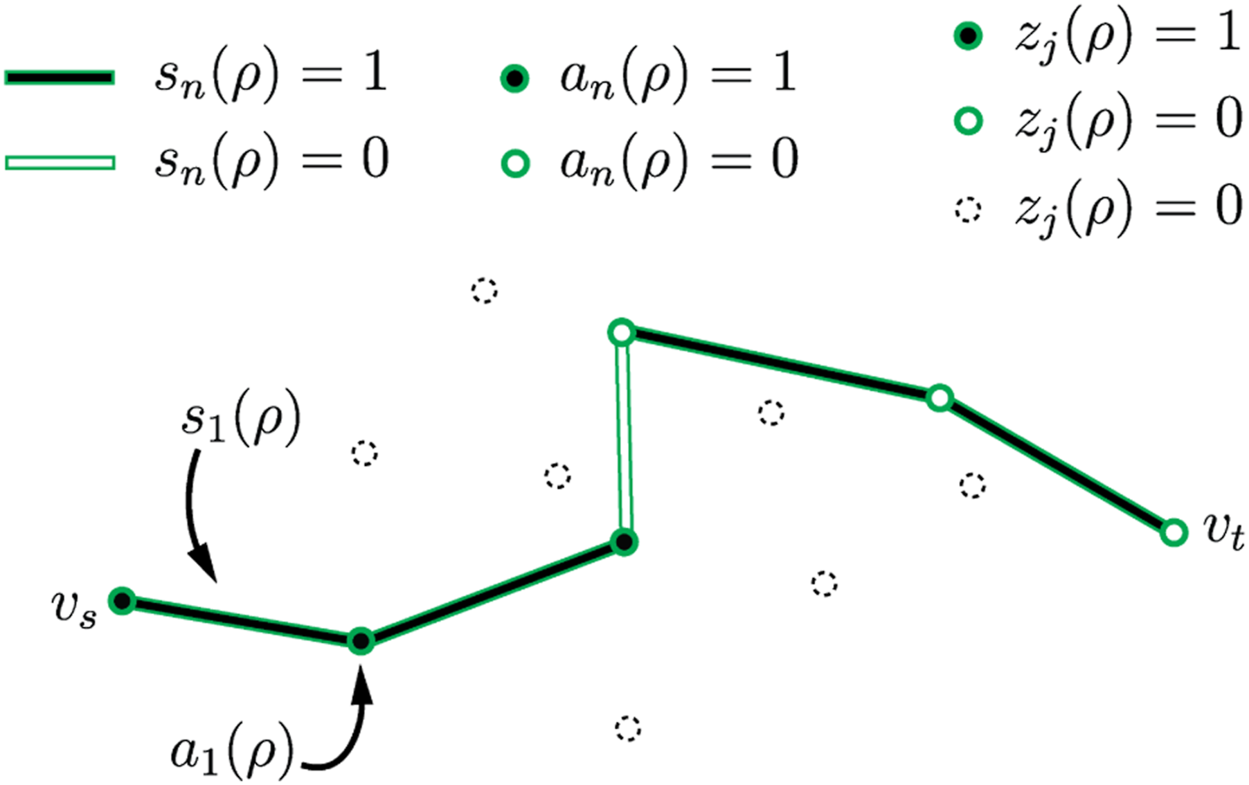

Given a start node v_s, a terminal node v_t, and survival probability p_s we must find at most K ≥ 1 paths ${ρ_{k}}_{k = 1}^{K}$ (one for each of K robots) such that, for all k, the probability that $a_{| ρ_{k} |}^{k} (ρ_{k}) = 1$ is at least p_s, ρ_k(0) = v_s and ρ_k(|ρ_k|) = v_t. The set of paths which satisfy these constraints is written as $X (p_{s}, ω)$ . One can test whether $X (p_{s}, ω)$ is empty with O(V² log(V)) computations using the method described in Jorgensen et al. (2018), so we assume that it is non-empty.

Define the indicator function $I {x}$ , which is 1 if x is true (or non-zero) and zero otherwise. Define the Bernoulli random variables for j = 1, …, V, k = 1, …, K:

z_{j}^{k} (ρ) : = \sum_{n = 1}^{| ρ |} a_{n}^{k} (ρ) I {ρ (n) = j},

which are 1 if robot k following path ρ visits node j and 0 otherwise (

z_{j}^{k} (ρ)

is binary because a path is defined as a unique set of nodes). Note that

z_{j}^{k} (ρ)

is independent of

z_{j}^{k^{'}} (ρ^{'})

for k ≠ k′. The number of times that node j is visited by robots following the paths

{ρ_{k}}_{k = 1}^{K}

is given by

\sum_{k = 1}^{K} z_{j}^{k} (ρ_{k})

, and we write the probability that exactly m robots visit node j as

p_{j} (m, {ρ_{k}}_{k = 1}^{K})

. In this paper we are primarily interested in the probability that no robots visit node j, which has the simple expression:

p_{j} (0, {ρ_{k}}_{k = 1}^{K}) = \prod_{k = 1}^{K} (1 - E [z_{j}^{k} (ρ_{k})]) .

Let d_j > 0 be the reward accumulated for visiting node j at least once, and define $X$ as the set containing K copies of each path in $X (p_{s}, ω)$ . Given a matroid $(X, I)$ with rank K, we are interested in finding an independent set which maximizes the weighted expected number of nodes visited. Since the objective is non-negative, monotone, and submodular (Jorgensen et al. 2018), we assume without loss of generality that the size of the optimizing set is K, and state the Matroid TSO problem formally:

Matroid TSO (MTSO) Problem: Given a graph $G$ , edge weights ω, survival probability threshold p_s and matroid $(X, I)$ , maximize the weighted expected number of nodes visited by at least one robot:

\begin{array}{l} \underset{{ρ_{k}}_{k = 1}^{K} \in I}{maximize} \sum_{j = 1}^{V} d_{j} (1 - p_{j} (0, {ρ_{k}}_{k = 1}^{K})) \\ \begin{array}{l} subjectto & P {a_{| ρ_{k} |}^{k} (ρ_{k}) = 1} \geq p_{s} & k = 1, \dots, K \\ ρ_{k} (0) = v_{s} & k = 1, \dots, K \\ ρ_{k} (| ρ_{k} |) = v_{t} & k = 1, \dots, K \end{array} \end{array}

The optimization is over the independent sets of the matroid, and the solution is a set of K paths. The objective represents the cumulative expected reward obtained by the robots following the selected paths. The first set of constraints enforces the survival probability, the second and third sets of constraints enforce the initial and final node constraints. Note that we can also consider an “unrooted” variant by adding a new start and end node which have zero-weight edges to all nodes in $G$ . Variants where each robot have non-homogeneous start or end nodes can be represented via a transversal matroid constraint, as described below.

The MTSO problem can be viewed as a set maximization problem with a matroid constraint, where the domain of optimization is the family of independent sets $I$ . Crucially, since the objective is a submodular function (Jorgensen et al. 2018), Theorem 1 implies that the greedily selected set of paths will achieve reward close to the optimum.

4. Examples and applications

In this section we highlight several examples of matroids and their applications in the context of the MTSO problem.

4.1. Uniform matroid

Given a positive integer K, the independent sets of a uniform matroid are all subsets of the ground set $X$ with at most K elements. Optimization with a uniform matroid constraint is equivalent to imposing cardinality constraints on the solution size, which is the standard TSO problem.

4.2. Binary matroid

Given a function $ϕ : X \to {0,1}^{M}$ , the independent sets of a binary matroid induced by ϕ are all subsets $X \subseteq X$ such that the vectors {ϕ(x)}_x∈X are linearly independent (if ϕ maps to a real vector we call this a linear matroid).

Application to coverage: Consider a setting where we require each robot to focus on a different region. Define the regions as M node subsets $S_{m} \subseteq V$ , and define the “focus” of a path as the index of the region which contains the most nodes of the path (with ties broken deterministically). Let m_ρ be the smallest index corresponding to a subset which path ρ focuses on, that is $| S_{m_{ρ}} \cap ρ | \geq | S_{m} \cap ρ |$ for m = 1, …, M. Now define ϕ(ρ) as the m_ρth canonical basis vector in $R^{M}$ . Requiring the solution to be an independent set of the binary matroid induced by ϕ and with ground set $X (p_{s}, ω)$ , enforces the desired diversity of focus.

4.3. Transversal matroid

Given subsets ${X_{m}}_{m = 1}^{M}$ of the ground set, the independent sets of the transversal matroid are all subsets X which are partial transversals of ${X_{m}}_{m = 1}^{M}$ . In other words, if $X \in I$ , we can assign each element x_i ∈ X a unique number m_i ∈ {1, …, M} such that $x_{i} \in X_{m_{i}}$ .

Application to coverage: Note that the coverage constraint from Section 4.2 can be represented via a transversal matroid.

Application to launch constraints: Consider a scenario where only one robot can start on each outgoing edge of v_s. This could arise, for example, when robots are aerial vehicles which must launch from runways, and only one can launch from a runway in each direction. Let N(v_s) be the set of nodes with an edge to v_s, and define the subsets $X_{m} = {ρ \in X (p_{s}, ω) ∣ ρ (1) = n_{m}}$ for n_m ∈ N(v_s). That is, we have one subset for each starting edge. Requiring that the solution is an independent set of the transversal matroid induced by ${X_{m}}_{m = 1}^{M}$ enforces the launch constraints.

Application to heterogeneous teams: Suppose we have M types of robots, a robot of type m has feasible path set $X_{m}$ , and that we can deploy at most K_m robots of type m. Requiring the solution to be an independent set of a transversal matroid induced by K_m copies of $X_{m}$ for m = 1, …, M enforces that no more than K_m robots of type m are selected.

Application to traffic constraints: Suppose we have a scenario with disjoint regions of interest, each robot may visit exactly one region, and each region has a traffic constraint which limits the number of agents which can visit it. We represent the regions by disjoint node sets $V_{m} \subset V$ and the number of agents allowed to visit region m by K_m. Define subgraph $G_{m}$ as the subgraph induced by the node set $V_{m}$ , and let $G_{m}$ correspond to the set of feasible paths in subgraph $G_{m}$ . Requiring that the solution is an independent set of a transversal matroid induced by K_m copies of the sets $X_{m}$ enforces the traffic constraint.

Application to risk constraints: Suppose we have M survival probability thresholds $p_{s}^{1} \leq \dots \leq p_{s}^{M}$ . This setting could arise when there is a constraint on the risk of many robot failures, but requiring uniform survival probability thresholds would be too conservative to visit all of the nodes. Then we can choose ${p_{s}^{m}}_{m = 1}^{M}$ in order to provide the necessary flexibility while still maintaining tight control on risk. Requiring the solution to be an independent set of the transversal matroid induced by ${X (p_{s}^{m}, ω)}_{m = 1}^{M}$ enforces the desired constraints.

4.4. Gammoid

Gammoids allow us to express (among other things) nested cardinality constraints such as “select up to N₁ elements with trait 1, and of those elements up to N₂ can have trait 2, and of those elements, …” A Gammoid is represented formally by defining a graph to represent the notion of independence (see Figure 3 for an example).

Figure 3.

Illustration of multi-partite graphs which form the gammoid described in Section 4.4. A subset 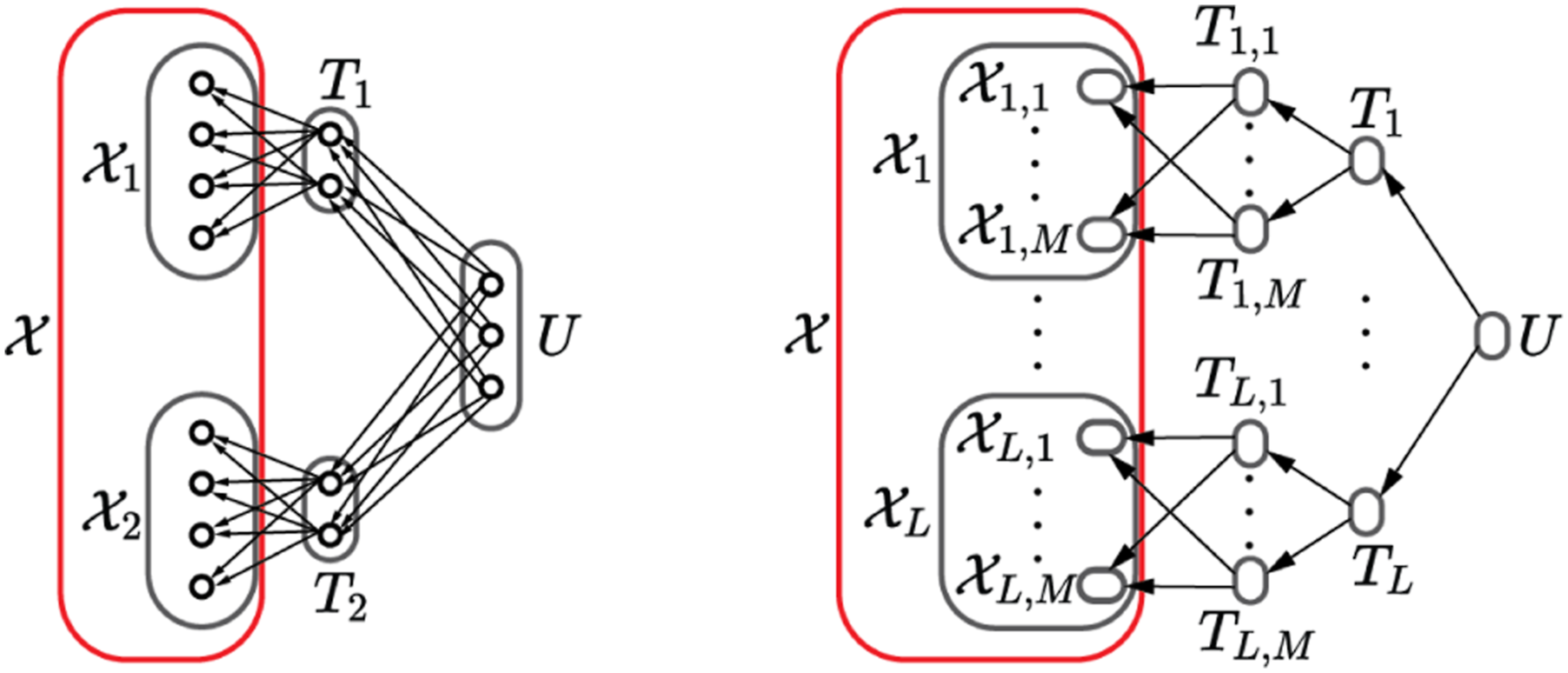$X \subseteq X$ is independent if there are node-disjoint paths from each element of X to elements of U (i.e., X is linked to U). Left: Two subsets $X_{1}$ , $X_{2}$ are connected to the subset U via nodes in T₁ and T₂. Since a path from $X_{1}$ must go through T₁ to reach U and T₁ only has two nodes, this means that we can only link two elements from $X_{1}$ to U (and similarly for $X_{2}$ ). Since U only has three nodes, we can only link 3 elements total from $X$ to U. Right: An illustration of the graph with three layers. Boxes represent clusters of nodes, and lines represent edges which connect each node of the right cluster to each node of the left cluster.

A gammoid is induced by a directed graph D(S, E) with a subset of nodes corresponding to elements in the ground set, for example, $X \subseteq S$ , and a subset U ⊆ S. We say that two sets of nodes X, Y ⊆ S are linked if |X| = |Y| and there are |X| node-disjoint paths from X to Y. The independent sets of a gammoid induced by D, U are all subsets $X \subseteq X$ such that some subset of U is linked to X.

Application to nested cardinality constraints: Consider a simple setting where the ground set is partitioned by the sets ${X_{1}, X_{2}}$ and we may choose up to 2 items from $X_{1}$ , 2 items from $X_{2}$ , and 3 items total. The independent sets of a gammoid induced by the multi-partite graph in Figure 3 satisfy these constraints. This setting is easily extended to more complicated scenarios. For the MTSO, we could first partition based on robot types, then by subgraphs, and finally by risk thresholds (or in a different order). An illustration of the graph for three layers of partitioning (e.g., robot types, subgraphs, and team size) is shown in Figure 3. It is not necessary for the node groups to form a partition.

This form of a gammoid is also known as a laminar matroid. It is important to note that this method of combining constraints is different from a matroid intersection—matroid intersections form a p-system and have weaker theoretical results described in Section 7.1.

4.5. Truncation

Given $K \in N$ and a matroid $(X, I)$ , let $I^{'} : = {I \in I ∣ | I | \leq K}$ which is the set of independent sets with at most K elements. Then $(X, I^{'})$ is a matroid and is called the K-truncation of $(X, I)$ . If the maximum team size is K, we can represent this constraint in addition to any of the scenarios above by using the K-truncation of the appropriate matroid.

5. Algorithms

In this section, we give greedy and accelerated continuous greedy approaches to solving the MTSO problem and give bounds on their suboptimality. Both algorithms solve single-robot sub-problems where a path from the feasible set is sought which approximately maximizes a path-dependent reward function. Accordingly we start by describing this sub-problem in detail in Section 5.1, which shows how to solve it as a series of orienteering problems, provides guarantees on the path quality, and a detailed discussion of implementation considerations for the examples given in Section 4. We then describe the greedy and accelerated continuous greedy approaches in Sections 5.2 and 5.3, respectively. Both of these sections describe how to form the appropriate sub-problem, the complete algorithm, performance guarantees, and computational complexity.

5.1. The greedy sub-problem

In this section we discuss the greedy sub-problem, giving a description of our solution approach in Section 5.1.1, discuss performance considerations in Sections 5.1.2, and its applications in Section 5.1.3.

5.1.1. Objective and algorithm

Given a (possibly empty) previously selected set of paths, $X_{L - 1} = {ρ_{l}}_{l = 1}^{L - 1}$ , the greedy sub-problem involves finding a path from the set $X_{F} (X_{L - 1}, I)$ which maximizes the sum of path-dependent node rewards ν(ρ, j) ≥ 0 corresponding to the discrete derivative of the appropriate objective function (we defer explicitly defining these objectives to Sections 5.2.1 and 5.3.1). Solving the greedy sub-problem is a critical step in both of our solution algorithms for the MTSO, but it is a very difficult task as it requires maximizing path-dependent node rewards subject to a budget constraint. Specifically, the path dependence is induced by the risky traversal model, since the reward gained for visiting node j depends on the probability that the robot successfully visits node j, which in turn depends on the path taken to the node. Furthermore, we must ensure that the path chosen is in $X_{F} (X_{L - 1}, I)$ .

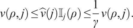
We address the path dependence by using a path independent approximation, $\hat{ν} (j)$ , of ν(ρ, j) which satisfies, for some γ ∈ (0, 1]:

ν (ρ, j) \leq \hat{ν} (j) I_{j} (ρ) \leq \frac{1}{γ} ν (ρ, j) .

We give concrete examples for computing $\hat{ν} (j)$ in Sections 5.2.1 and 5.3.1, but for now it suffices to view it as a scalar weight that satisfies the inequality given above.

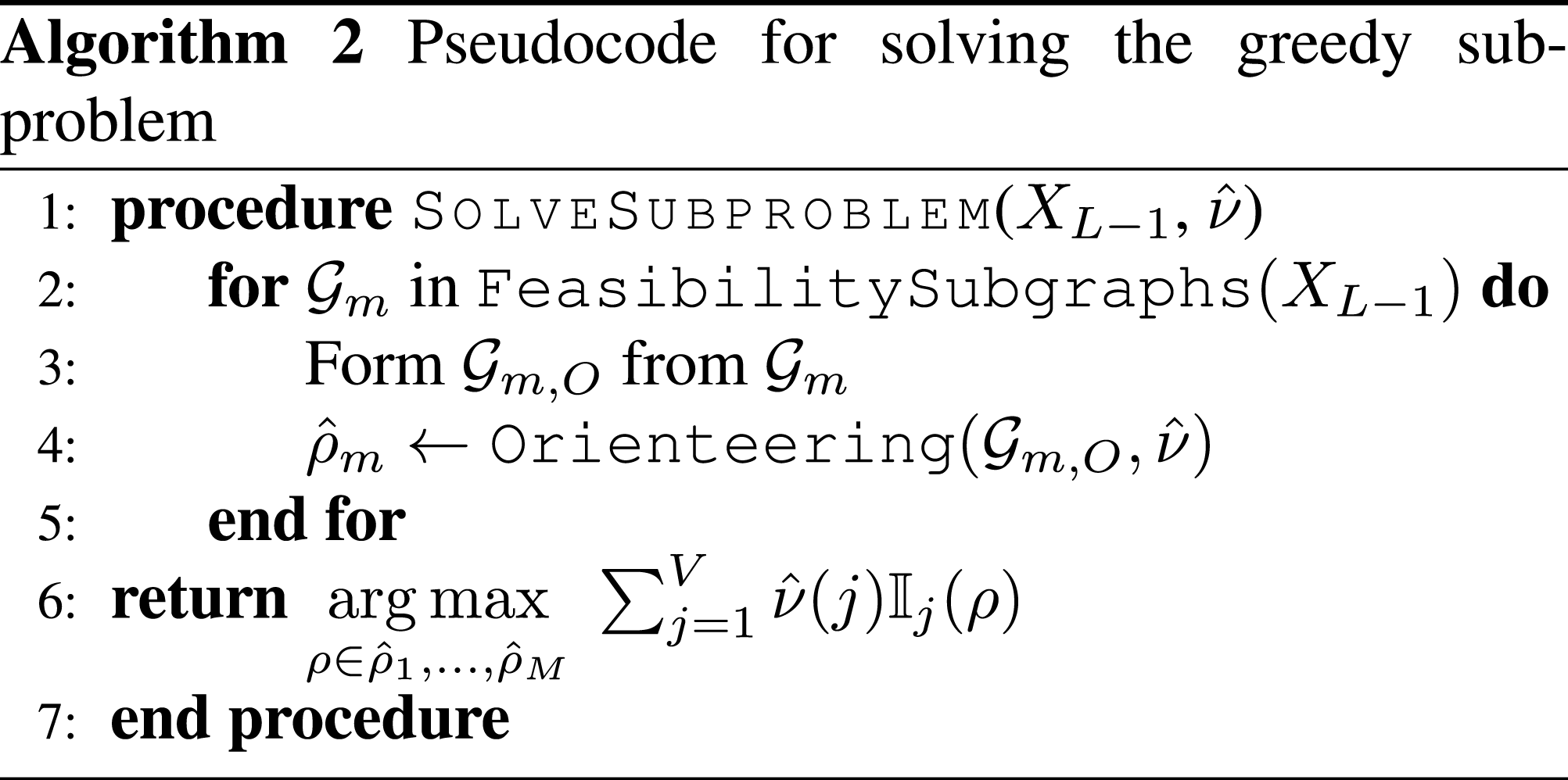
We address the matroid constraint by noting that the feasible set, $X_{F} (X_{L - 1}, I)$ , can always be decomposed into subsets of paths ${X_{m}}_{m = 1}^{M}$ where $X_{m}$ is the set of paths contained in subgraph $G_{m}$ . This is apparent from the fact that for each $ρ \in X_{F} (X_{L - 1}, I)$ , we can construct a subgraph $G_{ρ}$ which has exactly the nodes and edges in ρ. Since a path is defined as a unique list of nodes and edges, and since feasible paths must start at v_s and end at v_t, the subgraph $G_{ρ}$ contains only one feasible path, ρ. We provide procedures to construct a small set of subgraphs that cover $X_{F} (X_{L - 1}, I)$ for several relevant constraints in Section 5.1.3.

Our approach to solving the sub-problem is given as pseudocode in Algorithm 2. We begin by calling the $FeasibilitySubgraphs$ routine, which returns a list of subgraphs ${G_{m}}_{m = 1}^{M}$ which covers the feasible set $X_{F} (X_{L - 1}, I)$ . For each subgraph, we form a log-transformed graph $G_{m, O}$ which has edge weights ω_o = − log(ω). This graph and the approximate node reward $\hat{ν}$ are passed to an Orienteering oracle, which finds a path which has at least fraction 1/λ the optimal reward with edge costs at most B = − log(p_s) (we discuss this oracle in depth in Section 5.1.2). This ensures that the path is of high quality and satisfies the survival probability threshold constraint. Finally the routine returns the best of the paths computed (with respect to either $\hat{ν}$ or ν, depending how hard ν is to compute).

The following lemma guarantees that the path returned has similar value as the optimum:

Lemma 1

Sub-problem guarantee. Consider an MTSO problem with node weights d_j, let ρ be a feasible path in $X_{F} (X_{L - 1}, I)$ , and ${\hat{ρ}}_{L}$ be the path output by the SolveSubproblem routine described in Section 5.1.1. Then

\sum_{j = 1}^{V} d_{j} ν ({\hat{ρ}}_{L}, j) \geq \frac{γ}{λ} \sum_{j = 1}^{V} d_{j} ν (ρ, j) .

Proof

By definition of ${X_{m}}_{m = 1}^{M}$ , for any $ρ \in X_{F} (X_{L - 1}, I)$ there is a set indexed by m_ρ such that $ρ \in X_{m_{ρ}}$ . We have from the definitions of ${\hat{ρ}}_{L}$ , $\hat{ν} (ρ, j)$ , and the Orienteering routine:

\begin{array}{l} \sum_{j = 1}^{V} d_{j} ν (ρ, j) & \leq \sum_{j = 1}^{V} d_{j} I_{j} (ρ) \hat{ν} (j) \leq λ \sum_{j = 1}^{V} d_{j} I_{j} ({\hat{ρ}}_{L}) \hat{ν} (j) \\ \leq λ (\frac{1}{γ} \sum_{j = 1}^{V} d_{j} ν ({\hat{ρ}}_{L}, j)) . \end{array}

Suppose the computational complexity of the Orienteering routine given any subgraph is bounded by C_O, the complexity of the FeasibilitySubgraphs routine is bounded by C_F, and the FeasibilitySubgraphs routine returns at most M subgraphs. Then, the complexity of the SolveSubproblem routine is C_F + MC_O. We describe each of these terms in more detail below.

5.1.2. Complexity of the orienteering problem

Although the orienteering problem is NP-hard, various communities of researchers have developed solution approaches focusing on different properties of the solution—performance guarantees, on-line bounds, and run time. Depending on the oracle routine used, the SolveSubproblem routine has different guarantees and properties, namely,

Complexity theory guarantees—From a theoretical standpoint, if a polynomial time approximation scheme (PTAS) for the orienteering problem is used and the FeasibilitySubgraphs routine is polynomial time (meaning M is also polynomial), then our algorithm is a PTAS for the greedy sub-problem. Since our higher level routines call SolveSubproblem a polynomial number of times, this is a meaningful result on the complexity of the MTSO problem: although the MTSO is NP-hard, it can be approximated within a constant factor in polynomial time when there is an efficient FeasibilitySubgraphs routine. The complexity of the best known PTAS routines for the orienteering problem and its variants are high order polynomials—for example, Chen and Har-Peled (2006) gives a λ = 1 + ϵ PTAS for the case where points are on a d − dimensional plane that runs in $O (V^{16 d^{3 / 2} / ϵ})$ time. Even for ϵ = 1 and d = 2, this is O(V⁴⁶), which is not a practically useful bound.

Certifiable performance guarantees—Practitioners who require guarantees on the quality of the solution and more modeling flexibility can use mixed integer linear programming (MILP) formulations of the orienteering problem (e.g., Kara et al. (2016)). Commercial and open-source software for solving MILP problems are readily available, and return an optimality gap along with the solution. Such solvers can be configured to terminate after a set amount of time or when the ratio between the current solution and upper bound becomes greater than 1/λ.

Real-time properties—Finally, practitioners who require fast execution but not guarantees can use a heuristic to solve the orienteering problem. There are a number of fast, high quality heuristics with open-source implementations such as Wagner and Affenzeller (2005); Vansteenwegen et al. (2009). While these heuristics do not provide guarantees, they often produce near-optimal solutions and are capable of solving large problems in seconds.

5.1.3. Efficiently covering the feasible set

For many examples we can cover the feasible set using a small number of subgraphs, as detailed below. These descriptions are brief, but we also provide a GitHub repository with implementations for the following examples (ASL Github 2023).

Coverage—We can cover the sets for the coverage example by adding a constraint to a mixed integer formulation which requires the solution to have a specific focus. In this case M would be the number of regions to be covered.

Launch constraints—Given a set X_k, all paths which take edges (v_s, ρ_ℓ(1)), ℓ = 1, …, k are infeasible. Hence M = 1 and the subgraph is the graph induced by the edges $E^{'} = E ∖ {(v_{s}, ρ_{l} (1))}_{l = 1}^{k}$ .

Heterogeneous teams—The feasible sets are already covered by graphs $G_{m}$ corresponding to the graph that a robot of type m uses. Given a set X_k, the FeasibilitySubgraphs routine returns all subgraphs $G_{m}$ for which X_k has fewer than K_m paths.

Traffic constraints—Since the feasible path sets $X_{m}$ are disjoint, then the routine simply returns any subgraph $G_{m}$ for which X_k has fewer than K_m paths in $X_{m}$ . If the robot’s start location is not contained in the subgraph, then we need to encode the cost to reach the region of interest in the subgraph. This can be done by adding a new node to $G_{m}$ that is connected to all nodes in $V_{m}$ . The edge weights correspond to the cost to travel from the start node to the source node without going through any nodes in ${V_{m}}_{m = 1}^{M}$ , which we can get by solving a shortest path problem on the log-transformed graph. The complexity of solving the shortest path problem using Floyd-Warshall’s algorithm is the cube of the number of nodes and we do this for each of the subproblems, yielding a complexity of O(MV³).

Risk constraints—Given a set of paths X_k, the FeasibilitySubgraphs routine finds the smallest value $\hat{m}$ such that we can add a path with survival probability threshold $p_{s}^{\hat{m}}$ (this can be done naively with complexity O(M²)). Then the budget used by the Orienteering routine is set to $- \log (p_{s}^{\hat{m}})$ . Since the complexity of the orienteering routing depends strongly on graph cardinality, we can save compute by also computing the subgraph induced by the node set $V_{\hat{m}} : = {j \in {1, \dots, V} ∣ ζ_{j} \geq p_{s}^{\hat{m}}}$ , which are all nodes reachable within the desired survival probability threshold.

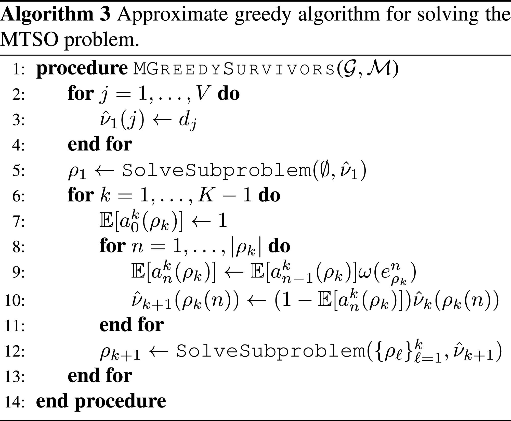
Nested cardinality constraints—Given a set of paths X_k, the FeasibilitySubgraphs routine tests whether a path can be added to each of the sets in the deepest layer (which partitions $X$ ). Then a subgraph corresponding to each of the subsets which we can still assign a path from is returned. The manner in which these subgraphs are computed depends on the application, as described in each of the sections above.

5.2. The approximate greedy algorithm

In this section we describe a greedy algorithm for solving the MTSO problem. We describe the objective function and detailed algorithm in Section 5.2.1, then give performance guarantees in Section 5.2.2, and characterize the complexity in Section 5.2.3.

5.2.1. Objective and algorithm

The greedy algorithm operates by iteratively selecting a path which maximizes the discrete derivative of the objective function for the MTSO given the set of previously chosen paths $X_{L - 1} \subset X$ . A node-wise decomposition of this objective was given in Jorgensen et al. (2018) as

Δ J (ρ ∣ X_{L - 1}) = \sum_{j = 1}^{V} d_{j} E [z_{j}^{L} (ρ)] p_{j} (0, X_{L - 1}),

which can be interpreted as the weighted sum over the probabilities that robots 1, …, L − 1 do not visit node j but robot L does. In the context of Lemma 1 we have

ν (ρ, j) = d_{j} E [z_{j}^{L} (ρ)] p_{j} (0, X_{L - 1})

, which can be approximated by setting

\hat{ν} (j) = d_{j} p_{j} (0, X_{L - 1})

, with γ = p_s. Pseudocode for the approximate greedy algorithm is given in Algorithm 3. The algorithm alternates between updating the approximate node rewards,

\hat{ν}

, and calling the SolveSubproblem routine to find an approximately optimal solution to the greedy sub-problem.

5.2.2. Guarantees

We combine the results from Section 2.3 and 5.1.1 to guarantee that the value of the output of Algorithm 3 is close to the value of the optimal solution to the MTSO problem.

Theorem 2

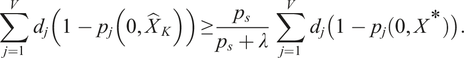
Approximate greedy guarantee. Let X* be an optimal solution to the MTSO problem, and ${\hat{X}}_{K}$ the set output by Algorithm 3. If the survival probability constraint is p_s and each orienteering sub-problem is solved within constant factor 1/λ, then the weighted expected number of nodes visited by a team of robots following the paths ${\hat{X}}_{K}$ is at least a fraction p_s/p_s + λ of the optimum, that is

\sum_{j = 1}^{V} d_{j} (1 - p_{j} (0, {\hat{X}}_{K})) \geq \frac{p_{s}}{p_{s} + λ} \sum_{j = 1}^{V} d_{j} (1 - p_{j} (0, X^{*})) .

Proof

Setting $ν (ρ, j) = E [z_{j}^{L} (ρ)] p_{j} (0, X_{L - 1})$ and $\hat{ν} (j) = p_{j} (0, X_{L - 1})$ , we have from Lemma 1 that the $SolveSubproblem$ routine solves the sub-problems within factor α = p_s/λ. Now, applying Theorem 1 to our objective function (which by Lemma 2 of Jorgensen et al. (2018) is normalized, non-negative, monotone, and submodular) we have the desired result.

In many scenarios robots are either valuable or difficult to replace, and so operators will choose survival probability thresholds p_s which are close to 1. Combined with an effective oracle routine, Theorem 2 guarantees that the greedy approach never collects less than approximately half of the optimal reward. This is a strong statement, since solving this problem optimally is extraordinarily difficult (especially as the team size grows).

5.2.3. Complexity

Algorithm 3 has complexity O(KV² + K(MC_O + C_P)), where the first term is the complexity of updating the V node weights K times (each update costs at most V multiplications), and the second term is the complexity of calling the $SolveSubproblem$ routine K times. In typical scenarios, the complexity will be dominated by KMC_O, as solving the orienteering problem is typically several orders of magnitude more difficult than decomposing the feasible set or updating the weights.

5.3. The accelerated continuous greedy algorithm

In this section we describe an accelerated continuous greedy algorithm for solving the MTSO problem. We begin by describing the objective function and detailed algorithm in Section 5.3.1, then give performance guarantees in Section 5.3.2 and characterize the complexity in Section 5.3.3.

5.3.1. Objective and algorithm

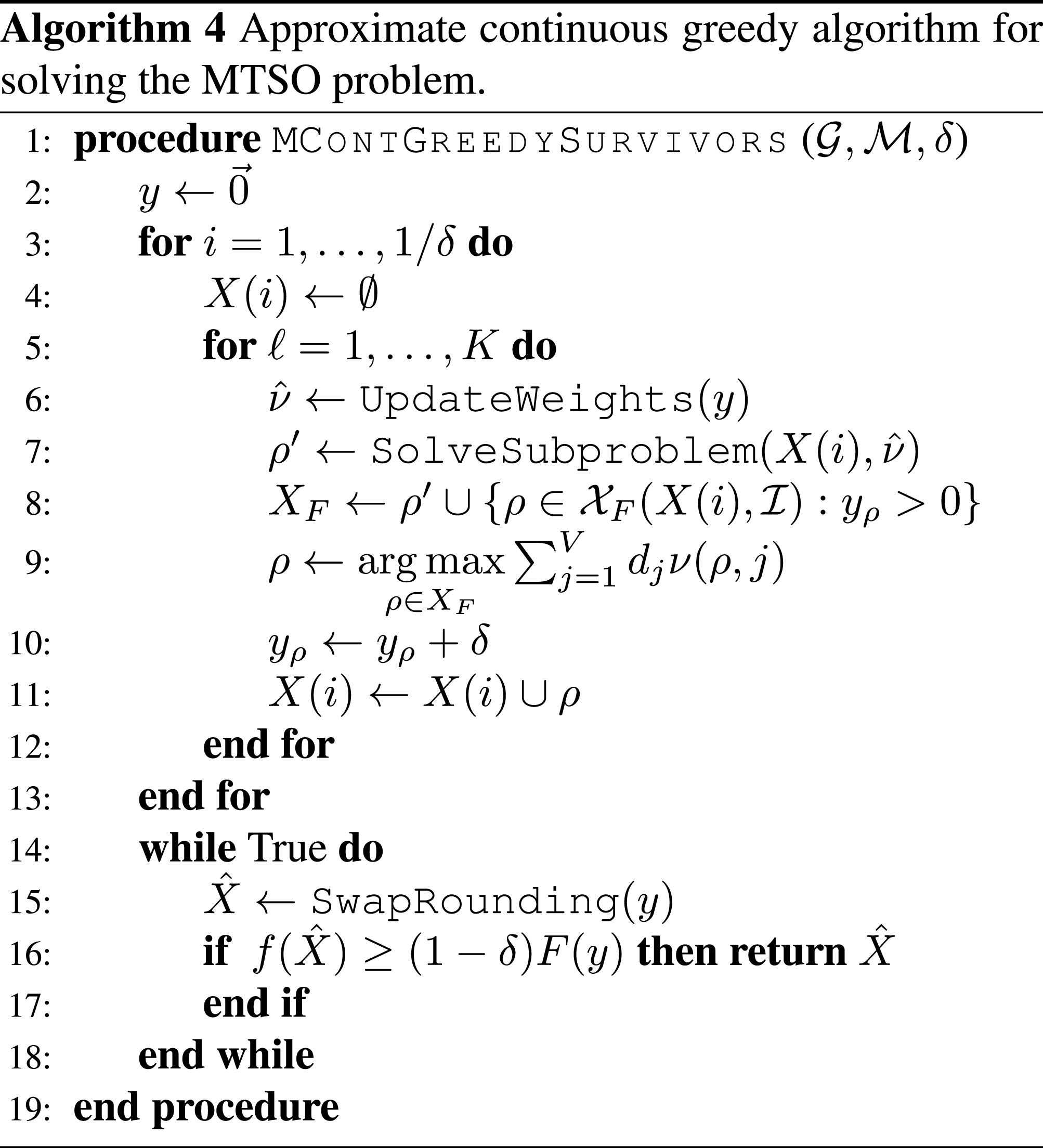
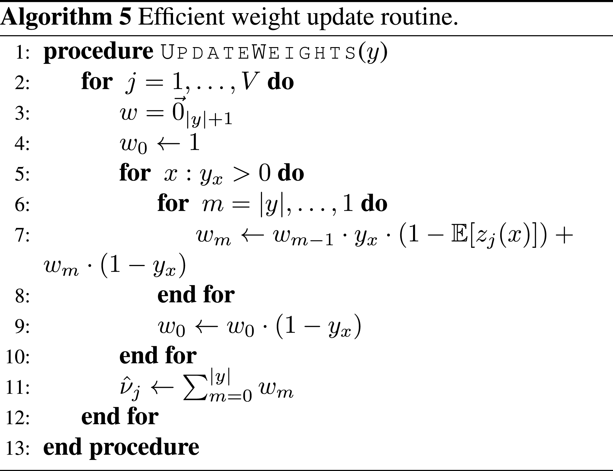
The accelerated continuous greedy algorithm (Badanidiyuru and Vondrák 2014) performs a discretized coordinate gradient ascent which optimizes the multilinear extension along “coordinates” corresponding to independent sets in the matroid. The state of the algorithm is given by a sparse vector $y \in {[0,1]}^{| X |}$ which can be interpreted as a probability distribution over elements in $X$ . The algorithm runs for $1 / δ \in Z_{+}$ steps (indexed by i), each consisting of K iterations (indexed by ℓ). During every iteration a single component of y corresponding to a path $ρ \in X$ is incremented by δ, that is y ← y + δ1_ρ where 1_ρ is the indicator vector which has all zero entries except the component corresponding to ρ, which is 1. The component ρ is selected to ensure that (1) the paths corresponding to the set of components updated in a given step are independent, and (2) the component approximately maximizes F(y + δ1_ρ) − F(y), which is equivalent to maximizing the discretized gradient with discretization step δ.

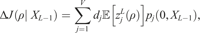
The objective for the ACGA can be written as an expectation with respect to the random set R(y), which contains elements in $X$ sampled independently with probability y_ρ, that is

P {R (y) = X} = \prod_{x \in X} y_{x} \prod_{x^{'} \in X^{c}} (1 - y_{x^{'}}) .

The following lemma gives an alternate expression for the objective in terms of a sum over path-dependent node rewards:

Lemma 2

Objective function for the ACGA. Let f be the objective of the MTSO and F its multilinear extension. The objective for the ACGA with state y during the ℓth iteration of the ith step can be written as

F (y + δ 1_{ρ}) - F (y) = δ \sum_{j = 1}^{V} \frac{d_{j} E [z_{j}^{ℓ} (ρ)]}{1 - y_{ρ} E [z_{j}^{ℓ} (ρ)]} E [p_{j} (0, R (y))] .

This result is derived directly from the definitions of the relevant variables (a detailed proof is given in the Appendix).

Pseudocode for our algorithm is given in Algorithm 4, which consists of three main parts: (1) efficiently computing $E [p_{j} (0, R (y))]$ , (2) removing path dependence for the sub-problem, and (3) rounding the solution. We discuss each part in detail below.

1) Efficiently computing $E [p_{j} (0, R (y))]$ : In general, computing an expectation over functions of the random set R(y) is difficult because the function must be evaluated for each of the 2^K/δ realizations of R(y). In our case, we exploit the product form of p_j(0, R(y)) to efficiently compute the expected value for fixed sizes of R(y), that is $E [p_{j} (0, R (y)) I {| R (y) | = m}]$ , which are then summed to compute the desired expectation. The algorithm is given in pseudocode in Algorithm 5, a complete implementation is provided in the GitHub repository (ASL Github 2023), and details on its correctness are given in the Appendix. The complexity of this approach is O(VK²δ⁻²).

2) Removing path dependence for the sub-problem: The objective is path-dependent because the term $E [z_{j} (ρ)] / 1 - y_{ρ} E [z_{j} (ρ)]$ depends on the probability that node j is visited (which is a function of the path taken) and the weight assigned to path ρ. We handle this term in two stages: we start by assuming that y_ρ = 0 (which is true for most paths) in which case we have $E [z_{j} (ρ)] / 1 - y_{ρ} E [z_{j} (ρ)] = E [z_{j} (ρ)]$ and use the strategies developed in Section 5.2.1 to approximately maximize the objective by solving an orienteering problem. We then compute the value of the O(K/δ) paths which have y_ρ > 0 (corresponding to the solutions to the greedy sub-problem in previous iterations) explicitly and select the better of these paths or the output of the orienteering routine solved in the first stage. We show in the Appendix that this two-stage approach produces a path with value within factor p_s/λ of the optimal.

3) Rounding the solution: We use the SwapRounding procedure to round y in order to get our final solution. In order to ensure that we achieve a good result we repeat the rounding procedure until the result is at least (1 − δ)F(y). The expected number of calls to the rounding routine is upper bounded by $1 / (1 - e^{- p_{s} δ^{2} / 8})$ , which is O(δ⁻²) (we defer details of these calculations to the Appendix).

Note that the set X_F is sparse because y has at most K/δ non-zero entries—the search over a large set of paths is encapsulated within the SolveSubproblem routine.

5.3.2. Guarantees

Combining our results from Sections 2.3, 5.1.1, and 5.3.1 we provide the following performance guarantee for Algorithm 4:

Theorem 3

Suboptimality bound. Let X* be an optimal solution to the MTSO problem and $\hat{X}$ be the output of Algorithm 4 routine with parameters δ and λ. Then the value of the set $\hat{X}$ is lower bounded by a constant factor of the optimum:

f (\hat{X}) \geq f (X^{*}) (1 - δ) (1 - \exp (- \frac{p_{s}}{λ + δ p_{s}})) .

The detailed proof is given in the Appendix. The basic idea is to first use the properties of the SolveSubproblem routine to lower bound the incremental increase in the multilinear extension between subsequent steps of the algorithm, then to use a recursive argument to show that F(y) satisfies the desired inequality, which in turn ensures that $f (\hat{X})$ satisfies the guarantee.

Tightness of the guarantee—As the approximation parameters converge to their ideals (δ → 0, λ → 1, p_s → 1), the guarantee converges to $f (\hat{X}) \geq f (X^{*}) (1 - e^{- 1})$ , which matches the hardness bounds for the general problem of maximizing a submodular function subject to a matroid constraint. We also note that for δ ≪ λ, the guarantee is approximately $1 - e^{- p_{s} / λ}$ , which matches the guarantee given for the TSO problem (Jorgensen et al. 2018).

5.3.3. Complexity

Algorithm 4 calls the UpdateWeights routine K/δ times, solves K/δ sub-problems, and calls the $SwapRounding$ routine an average of O(δ⁻²) times. Hence the total complexity is

O (δ^{- 1} K (M C_{O} + C_{P}) + δ^{- 3} K^{3} V + δ^{- 3} K),

and since generally C_O ≫ δ⁻²K²V, this is O(δ⁻¹KMC_O), which is a factor of δ⁻¹ greater than the approximate greedy routine.

6. Experimental results

In this section we validate and compare our solution approaches using simulations. In particular, we demonstrate the rich sets of constraints a matroid can model in Section 6.1, where we consider a challenging environmental monitoring scenario and compare two choices for the Orienteering oracle. Section 6.3 quantifies the empirical scaling of our algorithm using synthetic data. In particular, section 6.3.1 shows that Algorithm 3 scales as expected as the team size and number of sub-problems required to cover the feasible set grows, and Section 6.3.2 shows that the runtime of Algorithm 4 scales as expected with respect to δ. Finally, in Section 6.4 we compare Algorithm 3 and Algorithm 4 approaches for a range of δ values and discuss the strengths of each approach.

6.1. Environmental monitoring application

We consider the application illustrated in Figure 1: the Coral Triangle has a diverse ecosystem and the goal is to use a robotic fleet with multiple sensor configurations to monitor the wildlife populations in “Marine Protected Areas.” We use piracy incident data International Chamber of Commerce: Commercial Crime Services (2017) and model attacks as a Poisson random variable in a manner similar to Vaněk et al. (2013). We selected 106 marine protected areas from Cros et al. (2014) as nodes in a complete graph and computed the shortest (minimum risk) paths between each pair of sites to find the edge weights. In our scenario, we can deploy up to 25 robots of three types (at most twelve of each type), and each robot type has a different utility in each region. Each region can support the traffic of at most three robots of each type.

We require that the expected losses over the worst 5% of outcomes be no more than five failed robots (this is called the Conditional Value at Risk, and denoted CVaR_0.05). For the data shown, the most difficult node to reach requires survival probability 0.64, but if we use a uniform survival probability threshold p_s = 0.64, the risk is unacceptably high (CVaR_0.05 = 16.26). We satisfy the constraint CVaR_0.05 ≤ 5 by setting $p_{s}^{1}, \dots, p_{s}^{5} = 0.6$ , and $p_{s}^{6}, \dots, p_{s}^{25} = 0.859$ , that is, we allow five robots to take more risky paths and constrain the rest to more conservative paths. All of the constraints above can be represented using a single gammoid, and the feasible set can be covered using at most M = 15 subgraphs. Note how expressive gammoids are—this example uses just three levels of “nested constraints” (robot types, traffic limits, and risk constraints) but we could easily use more.

We consider two choices for the Orienteering routine: an open-source Variable Neighborhood Search (VNS) heuristic produced by HeuristicLab (Wagner and Affenzeller 2005) and a mixed integer linear program (MILP) formulation solved using CPLEX with a 5% tolerance. We observe that the VNS heuristic gives near-optimal paths, and solves all of the sub-problems for each of the twenty five robots in 51 seconds on a quad-core 4GHz processor with 32GB RAM available. The MIP oracle takes 60 seconds and yields nearly the same results. While the MIP oracle can find high quality paths quickly, as the tolerance is decreased the computation time dramatically increases. Optimally solving the sub-problems does not necessarily lead to better overall behavior, as shown in Figure 4. The upper bound shown is computed as the smaller of 1) the upper bound found using the greedily selected paths and the approximation ratio, and 2) the sum of all node rewards $\sum_{j = 1}^{V} d_{j} = 106$ . This upper bound is loose because it ignores the constraints (particularly on the traffic flow through a region) which becomes apparent as the team size grows larger. Note that although the theoretical approximation guarantee is 0.36, a team of 10 robots achieves 0.928 the maximum possible reward, despite only planning one path at a time.

Figure 4.

Cumulative reward for paths planned by Algorithm 3 using the MIP and VNS Orienteering routines. Both approaches compute high quality sets of paths, though VNS is somewhat faster.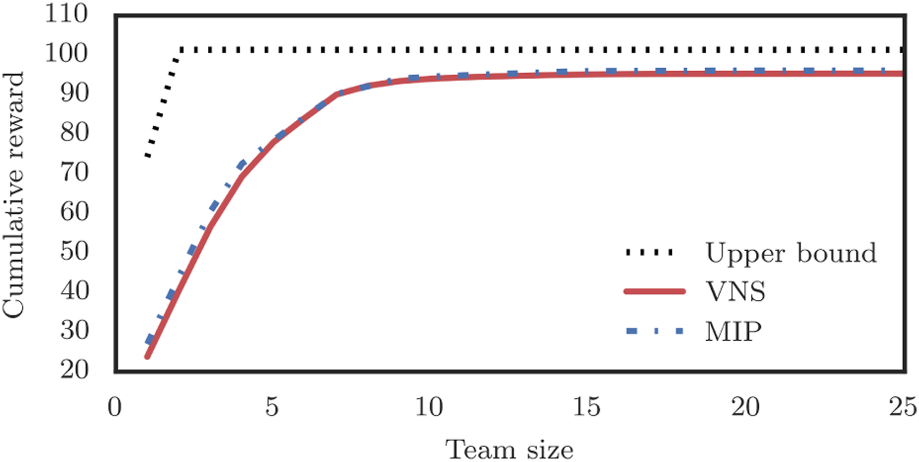

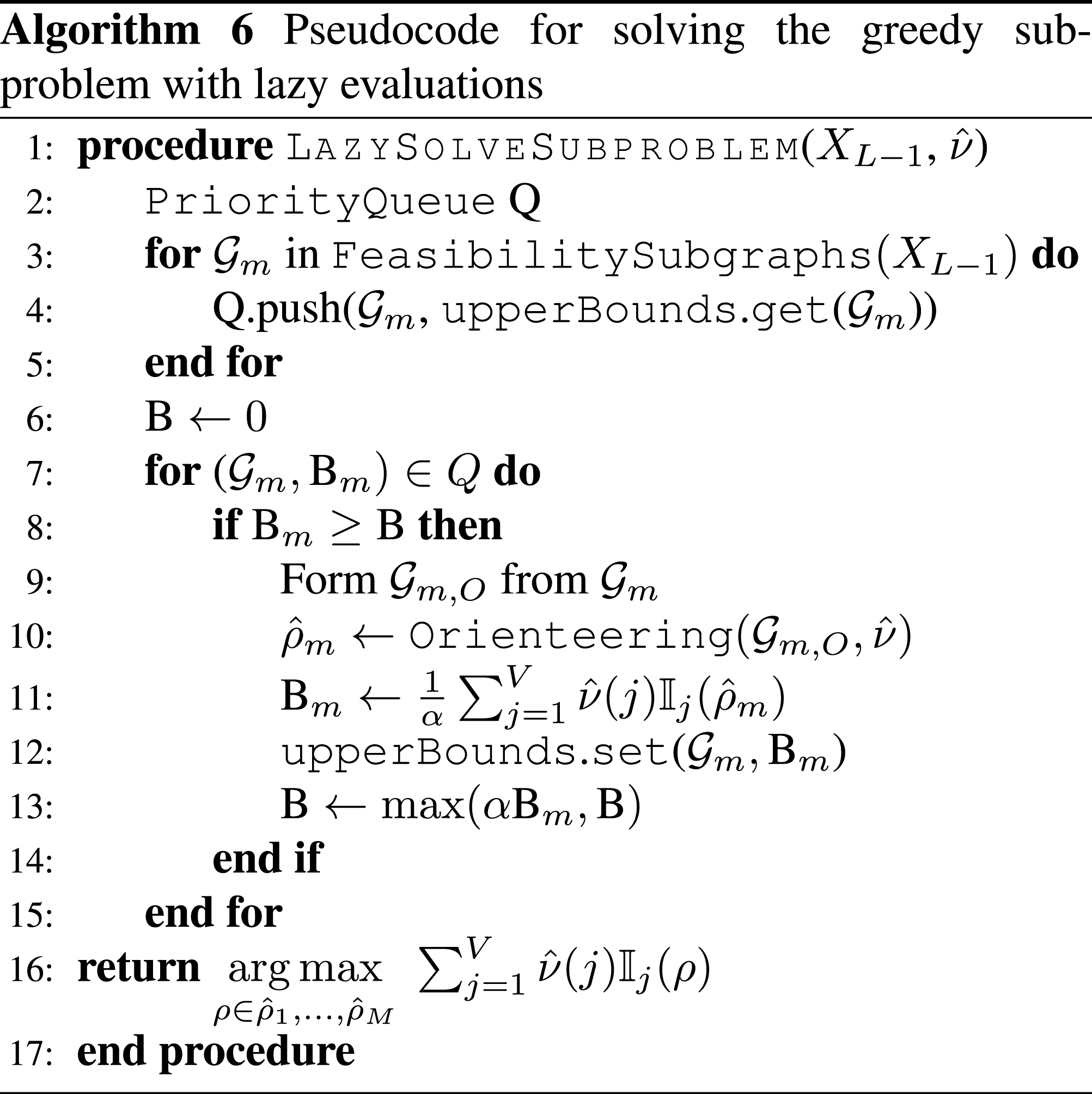
6.2. Lazy evaluations

Lazy evaluation (Krause and Golovin 2014) is an important practical modification to submodular maximization algorithms. Each time an orienteering problem is solved, we can use the optimality gap from the solver to bound the maximum reward of any path in the subgraph. Since the value of a path is a decreasing function as the algorithm progresses (due to submodularity), these bounds can be used in the following iterations.

We implement this LazySolveSubproblem routine by adding a priority queue to sort subgraphs based on their upper bounds, and a database to track the upper bounds between calls to LazySolveSubproblem. Let upperBounds be a persistent map data structure with method set(key, value) which assigns the value associated with the key, and method get(key) that returns the stored value for that key or ∞ if no value is stored. The pseudocode for this approach is given in Algorithm 6 and a more detailed example is provided in the GitHub repository (ASL Github 2023).

6.3. Synthetic problem generation

We demonstrate the scaling properties of Algorithm 3 and Algorithm 4 using synthetic data. Nodes are placed randomly on a 2D plane and clustered into groups of 15-20 nodes. This ensures the complexity of solving the orienteering problem, C_O, is constant and allows our analysis to focus on the other aspects of our algorithm. We refer readers interested in the complexity of the orienteering problem to the literature in Section 5.1.2 which treat the subject in detail.

We consider a traffic constraint with subgraphs induced by the clusters. Edge weights are chosen so that −log(ω(e)) is proportional to the length of the edge e, the survival probability threshold is set to 0.7, and we use a MILP formulation for the planar orienteering problem with tolerance 5%. An illustration of the paths selected for one instance is shown in Figure 5

Figure 5.

Illustration of a set of paths produced by our algorithm for a synthetic data set. Colors are used to distinguish paths taken by different robots (the lines) and nodes in different regions (the dots).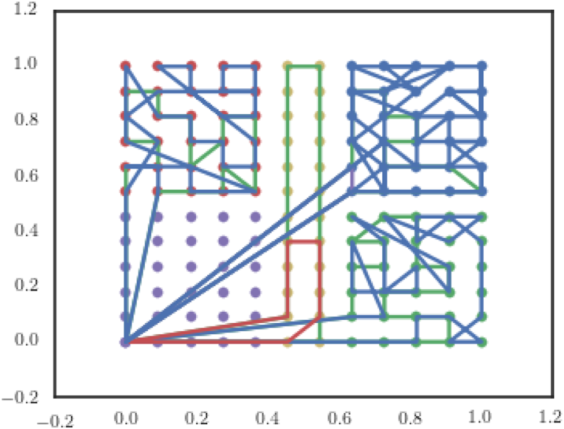

6.3.1. Sub-problem complexity scaling

We demonstrate the complexity of the Algorithm 3 with respect to K and M using the synthetic dataset described above. Using the lazy evaluation strategy described in Section 6.2 allows us to skip 75% of the sub-problems in this experiment. The median computation times are shown in Figure 6.

Figure 6.

Scaling of Algorithm 3 as K and V grow. Data shown is the median of 110 samples, and agrees with an Θ(MKC_O) trend.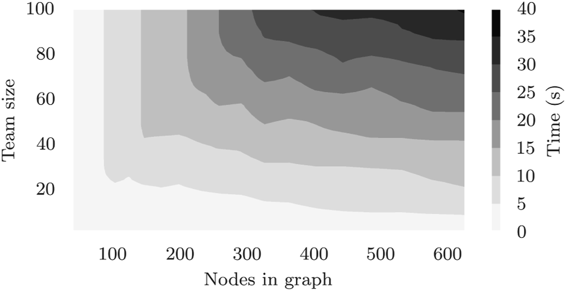

The complexity analysis from Section 5.2.3 suggests that since C_O is constant, compute should scale as the product MK. The x-axis in Figure 6 is proportional to M, and the y-axis is proportional to K. A visual comparison of this figure with a contour plot off(x, y) = xy verifies that the compute scaling is consistent with the predicted O(MKC_O) complexity.

For this size of sub-problem our approach solves large problems with very large teams in under a minute—the reasons for this are threefold: First, any given subgraph has a small size; Second, we permit the solver to terminate once it finds a solution within 5% of the optimal; and Third, we are using a high performance solver (Gurobi). In practice there are many approaches to solving the underlying orienteering problems (as discussed in Section 5.1.2) and solvers should be tuned to the hardware and particulars of an application, so these figures should be viewed as a baseline.

6.3.2. Discretization complexity scaling

As discussed in Section 5.3.3, we expect the run time of Algorithm 4 to be roughly δ⁻¹ times that of Algorithm 3 (which is Algorithm 4 with δ = 1). We demonstrate this trend empirically by using the synthetic data generated as described at the beginning of this section (with V = 82 and K = 8). For each problem we compute the baseline by averaging the run time of 5 calls to Algorithm 3. We then measure the run times of Algorithm 4 with the desired δ values and use the ratio of Algorithm 4 run times to the baseline run time as our datapoints. We repeated this for 30 randomly generated problems and show the results in Figure 7. The randomness in run times is due to several factors (1) lazy implementation allows for problems to be skipped when good bounds are available, (2) MIP solver time can depend significantly on the particular problem, and (3) MIP solver times are not deterministic.

Figure 7.

Scaling of the run time of Algorithm 4 relative to Algorithm 3 as the number of discretization steps increases. Note that run time increases approximately linearly with δ⁻¹, as predicted in Section 5.3.3.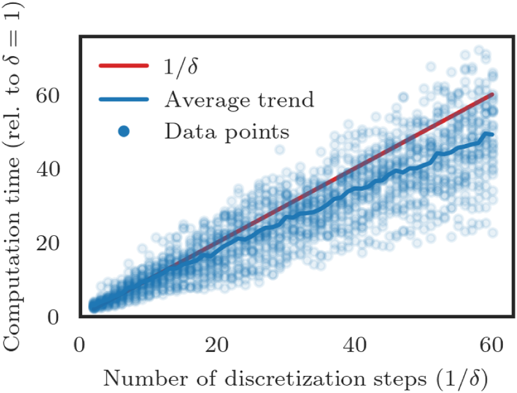

6.4. Effect of discretization on performance

Using the same data as in Section 6.3.2, we analyze the influence of the discretization parameter on the performance of Algorithm 4 relative to Algorithm 3 in terms of the value of their solutions. As shown in Figure 8, increasing δ⁻¹ generally improves the performance, and generally increases the chance that the result produced by Algorithm 4 will be better than the result produced by Algorithm 3. Note that the benefits of smaller discretization sizes drop off faster than the increase in computation time, so in practice a relatively small value of δ⁻¹ (e.g., 8 or 16) should be used. In scenarios where computation time is paramount, Algorithm 3 provides a fast way of achieving high quality solutions.

Figure 8.

Comparison of objective achieved by Algorithm 4 and Algorithm 3 with δ⁻¹ ∈ {2, …, 60} for 30 random MTSO problems. Note that as δ⁻¹ increases the Algorithm 4 more consistently outperforms the baseline and average performance increases.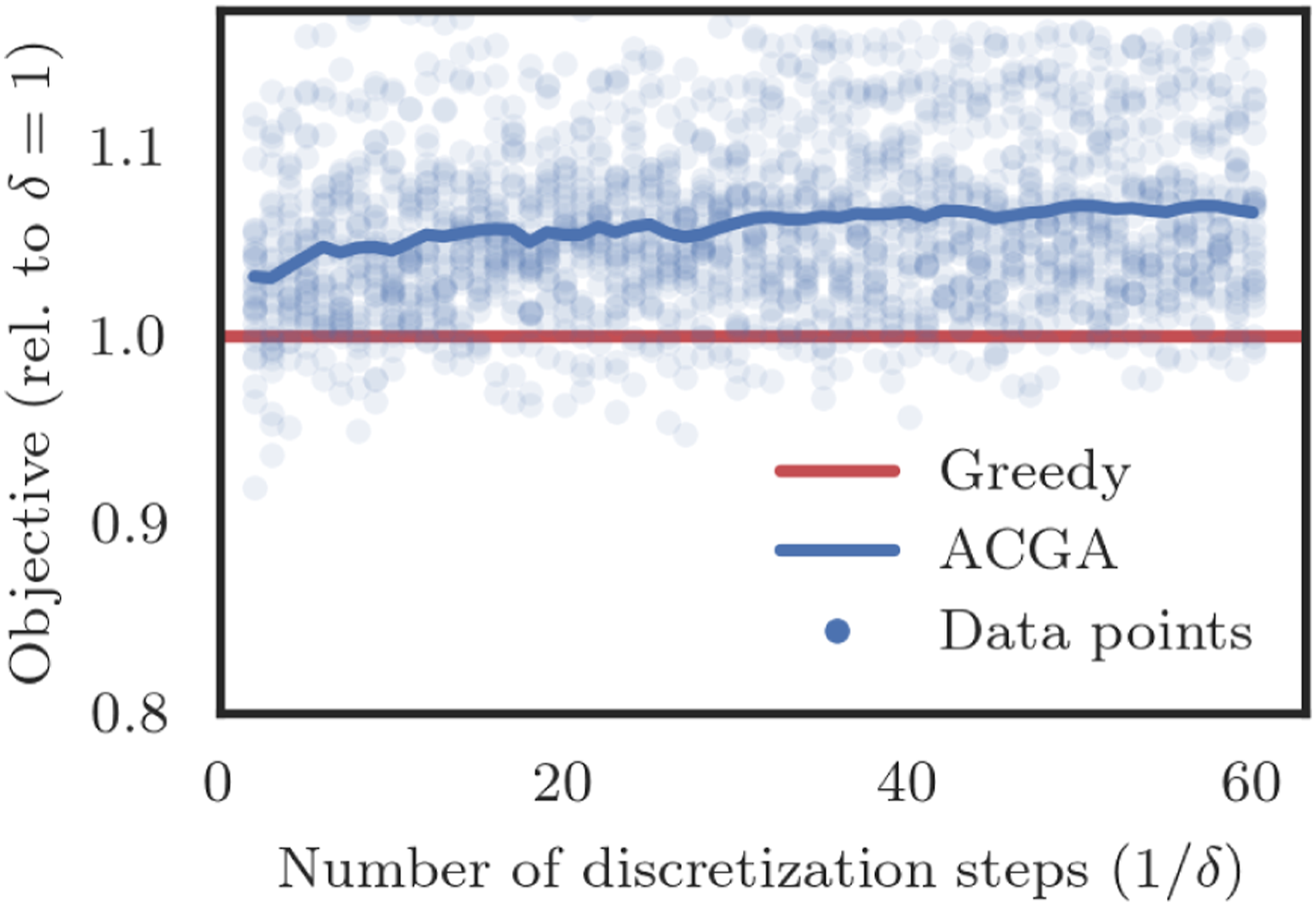

7. Extensions

In this section we discuss additional extensions and applications of our work. In Section 7.1, we describe p-systems and their applications to robotics. Minor modifications to algorithms presented above have constant factor guarantees for p-systems. In Section 7.2 we describe the coverage variant of the MTSO, which is closely related to our other work in Jorgensen et al. (2017b). Results from Chekuri et al. (2010) can be applied to provide guarantees for Algorithm 4 in this setting.

7.1. p-system constraints

Consider the MTSO where the matroid $M$ is replaced by a p-system. Recall that a p-system is an independence system which is downward closed and every base (maximal independent set) has at most p elements. The crucial distinction between p-systems and matroids is that the latter has the exchange property, which implies that every base in a matroid has the same number of elements (which is the rank of the matroid).

7.1.1. Applications to robotics

Many common constraints in robotics can be modeled as a p-system:

Collision avoidance—Consider a setting where we do not allow two robots to simultaneously traverse the same edge in the graph (this also requires us to introduce a notion of time, which we discuss more in our work Jorgensen et al. (2018)). One can easily verify that collision avoidance is downward closed—any subset of a set of collision free paths will also be collision free. The value of p is easily bounded by the smaller of the out-degree of the starting vertex and the number of robots allowed.

Capacity constraints—Collision avoidance can be generalized to a capacity constraint, where each edge has a capacity, and each robot has a demand. We can require that the sum of demands for robots simultaneously traversing an edge must be below the capacity of the edge. Note that collision avoidance is a special case where all demands and capacities are equal. This scenario can model road networks as well as communications networks, where a video sensor may demand much more bandwidth than other types of sensors.

Matroid intersections—The intersection of p matroids is also a p-system. This can allow us to simultaneously enforce risk constraints, sensor availability, and traffic constraints. Note that this is different from the nested cardinality constraints used in the experiments. For example, we could require that at most 5 of the 25 paths planned are risky and that at most 12 of each robot type can be selected (rather than the nested case, which would say, e.g., at most 12 of the risky paths can be of a given type, and at most 12 of the safe paths can be of a given type).

7.1.2. Algorithms and guarantees

We can use a slightly modified version of our algorithms above to find a set which is in the independent family of sets for a p-system and (approximately) maximizes the expected number of nodes visited. The only difference is that now the feasible set $X_{F} (X, I)$ is defined with respect to the independent family of sets for a p-system. A similar application-specific FeasibilitySubgraphs technique can be used in the SolveSubproblem routine.

The guarantee we state in Theorem 1 is a special case of the more general statement from Appendix B of Calinescu et al. (2007), which for a p-system gives the constant factor guarantee α/α + p. For our applications, we will typically constrain teams to have at most K robots which implies p ≤ K (since no set can have more than K elements). Using α = p_s/λ this means that the guarantee can be written as p_s/p_s + Kλ, which while a constant factor, quickly becomes loose as the team size grows.

7.2. Multiple objectives and coverage problems

Consider a problem where we are given a set of submodular functions f₁, …, f_N, corresponding values V₁, …, V_N, and want to find a set X such that f_n(X) ≥ V_n for n = 1, …, N.

7.2.1. Applications to robotics

This problem could model a coverage variant of the MTSO, where we are seeking a set X which satisfies a matroid constraint while also ensuring that the probability node j is visited satisfies a given threshold, p_v(j). In this setting we define the functions f_j(X) = min{1 − p_j(0, X), p_v(j)} and set V_j = p_v(j). This is similar to the coverage variant of the TSO given in Jorgensen et al. (2017b), where we seek the smallest team which satisfies the desired visit probabilities.

7.2.2. Algorithm and guarantees

The algorithm for this case only requires minor modifications to our proposed algorithms, and would leverage the modifications to the continuous greedy algorithm outlined in Chekuri et al. (2010). Theorem 2.5 from Chekuri et al. (2010) guarantees that the output of the modified algorithm satisfies F_n(y) ≥ (1 − e⁻¹)V_n for n = 1, …, N, or returns a certificate of infeasibility. In our case Algorithm 4 has a weaker $1 - e^{- p_{s} / λ}$ guarantee, and so the result would be modified accordingly. If the visit probability thresholds are small enough, we can guarantee feasibility by dividing V_j by $(1 - e^{- p_{s} / λ})$ , ensuring that the visit probability is greater than p_v(j).

8. Conclusions

8.1. Summary

We formulate the Matroid Team Surviving Orienteers (MTSO) problem, where we seek a set of paths which forms an independent set of a matroid, maximizes the expected number of nodes visited by at least one robot, and ensures the probabilities each robot reaches its destination are above a threshold. This problem is a significant generalization of our earlier work on the Team Surviving Orienteers problem (Jorgensen et al. 2018), and is distinct from previous work because it combines a submodular objective, chance constraints, and matroid constraints. We give numerous applications of matroids to robotic path planning such as coverage, launch constraints, limits on the number of available robots of multiple types, restrictions on the amount of traffic which can flow through a region, and combinations of the above. The MTSO is particularly challenging to solve because of the risky traversal model (where a robot might not complete its planned path) which creates a complex, history-dependent coupling between the edges chosen and the distribution of nodes visited. We present two solution algorithms: an approximate greedy algorithm for solving the MTSO problem which guarantees that its output achieves at least $\frac{p_{s}}{p_{s} + λ}$ of the optimal reward, and a variant of the ACGA which guarantees that its output achieves at least $≃ 1 - e^{- p_{s} / λ}$ the optimal reward. The algorithms rely on a FeasibilitySubgraphs routine to satisfy the matroid constraints, and we show numerous examples where our algorithm runs in polynomial time. We demonstrate the efficiency of our approaches by applying it to a scenario where a team of robots must gather information while avoiding pirates in the Coral Triangle, and study how algorithm parameters influence complexity and performance.

8.2. Future work

There are many directions for future work beyond those outlined in Section 7. The most promising is the extension to linear packing constraints (also called knapsack constraints). The multiplicative weight update (MWU) framework was used by Chekuri et al. (2015) to find a set X which optimizes a submodular function subject to linear packing constraints, 1_XA ≤ 1, where A is an $M \times | X |$ matrix. These constraints generalize common cases of matroid constraints, such as the partition, transversal, and laminar matroids, and can represent more general versions of the applications from Section 4 such as constraining the expected number of failures, the total number of types of sensors available, or limits on traffic through each edge in the graph. The MWU framework solves a cost-benefit greedy variant of the ACGA, where paths are weighted by their cost (i.e., how much of the constraint they use). Specifically, the algorithm increments the coordinate of y which ensures that the coordinates selected in a particular step satisfy the packing constraints, and which maximizes. In principle this is not much more difficult than Algorithm 4 presented in this paper, however, in practice this will require clever tailoring of the MILP formulations and careful selection of the constraint function to ensure that it can be solved as an orienteering problem (or that a suitable oracle routine exists). The FeasibilitySubgraphs routine will also need to be updated to represent the feasible space correctly. The guarantees for the MWU approach are very similar to those of Algorithm 4 and borrow the same arguments, so in principle we should expect similar results as given in Theorem 3, however, appropriately rounding the fractional solution remains an open problem. A second area for future investigation is distributed algorithms, which tend to be preferred over centralized algorithms for field robotics due to their resilience and lower compute requirements. Algorithms 3 and 4 both assume that computation is done on a centralized server. Corah and Michael (2019) showed an approach for running the sequential greedy algorithm in a distributed fashion to take advantage of parallel computation when communications are available. Extending these results for Algorithm 3 is straightforward, as it is also based on the sequential greedy algorithm. Extending Algorithm 4 would take more care but would be similar to the approach taken by Segui-Gasco (2017) and Robey et al. (2021). In both cases there is a trade-off between compute, time, and guarantees. A third direction for future work is to investigate notions of abstract dependence such as antimatroids, which can model queueing networks or precedence constraints. There are few fundamental results on optimizing with such abstract dependence constraints, but it is an active area of research and there are some recent results for the special case of “bottleneck functions” which may be useful in robotics.

\frac{1}{\sum_{m = 1}^{M} w_{m} A_{m, ρ}} (F (y + δ 1_{ρ}) - F (y)),

where w_m is a second state vector used for constraint satisfaction.

Footnotes

Acknowledgments

The authors would like to thank Jan Vondrák for helpful discussions about the accelerated continuous greedy algorithm and multilinear extension which started this work. The authors are also grateful to Robert H. Chen and Mark B. Milam for their contributions to the conference version of this work.

Declaration of Conflicting Interests

The author(s) declared no potential conflicts of interest with respect to the research, authorship, and/or publication of this article.

Funding

The author(s) disclosed receipt of the following financial support for the research, authorship, and/or publication of this article: This work was supported by the National Science Foundation (DGE-114747).

ORCID iD

Stefan Jorgensen

Appendix

References

ASL Github (2023) MTSOExamplesIJRR23. Available at https://github.com/StanfordASL/MTSOExamplesIJRR23

Atanasov

Le Ny

Daniilidis

, et al. (2015) Decentralized active information aquisition: theory and application to multi-robot SLAM. In: Proc. IEEE Conf. On Robotics and Automation. Piscataway, NJ: IEEE.

Badanidiyuru

Vondrák

(2014) Fast algorithms for maximizing submodular functions. In: ACM-SIAM Symp. On Discrete Algorithms. New York, NY: ACM.

Calinescu

Chekuri

Pál

, et al. (2007) Maximizing a submodular set function subject to a matroid constraint. In:Int. Conf. On Integer Programming and Combinatorial Optimization, Madison, WI, 2007.

Campbell

Gendreau

Thomas

(2011) The orienteering problem with stochastic travel and service times. Annals of Operations Research 186(1): 61–81.

Chekuri

Pál

(2005) A recursive greedy algorithm for walks in directed graphs. In: IEEE Symp. On Foundations of Computer Science. Piscataway, NJ: IEEE.

Chekuri

Vondrák

Zenklusen

(2010) Dependent randomized rounding via exchange properties of combinatorial structures. In: IEEE Symp. On Foundations of Computer Science. Piscataway, NJ: IEEE.

Chekuri

Jayram

Vondrák

(2015) On multiplicative weight updates for concave and submodular function maximization. In: Conf. On Innovations in Theoretical Computer Science. New York, NY: ACM.

Chen

Har-Peled

(2006) The orienteering problem in the plane revisited. In: ACM Symp. On Computational Geometry. New York, NY: ACM.

10.

Corah

Michael

(2019) Distributed matroid-constrained submodular maximization for multi-robot exploration: theory and practice. Autonomous Robots 43(2): 485–501.

11.

Cros

Ahamad Fatan

White

, et al. (2014) The Coral Triangle Atlas: an integrated online spatial database system for improving coral reef management. PLoS One 9(6): 1–7.

12.

Fisher

Nemhauser

Wolsey

(1978) An analysis of approximations for maximizing submodular set functions –II. In: Polyhedral Combinatorics. Springer.

13.

Golden

Levy

Vohra

(1987) The orienteering problem. Naval Research Logistics 34(3): 307–318.

14.

Gunawan

Lau

Vansteenwegen

(2016) Orienteering problem: a survey of recent variants, solution approaches and applications. European Journal of Operational Research 255(2): 315–332.

15.

Gupta

Krishnaswamy

Nagarajan

, et al. (2012) Approximation algorithms for stochastic orienteering. In: ACM-SIAM Symp. On Discrete Algorithms. New York, NY: ACM.

16.

Hoff

Andersson

Christiansen

, et al. (2010) Industrial aspects and literature survey: fleet composition and routing. Computers & Operations Research 37(12): 2041–2061.

17.

International Chamber of Commerce: Commercial Crime Services (2017) IMB piracy reporting centre. Available at https://www.icc-ccs.org/piracy-reporting-centre.

18.

Jawaid

Smith

(2015) Informative path planning as a maximum travelling salesman problem with submodular rewards. Discrete Applied Mathematics 186: 112–127.

19.

Jorgensen

Chen

Milam

, et al. (2017a) The matroid team surviving orienteers problem: constrained routing of heterogeneous teams with risky traversal. In: IEEE/RSJ Int. Conf. On Intelligent Robots & Systems. Piscataway, NJ: IEEE.

20.

Jorgensen

Chen

Milam

, et al. (2017b) The risk-sensitive coverage problem: multi-robot routing under uncertainty with service level and survival constraints. In: Proc. IEEE Conf. on Decision and Control. Piscataway, NJ: IEEE.

21.

Jorgensen

Chen

Milam

, et al. (2018) The team surviving orienteers problem: routing teams of robots in uncertain environments with survival constraints. Autonomous Robots 42(4): 927–952.

22.

Kara

Biçakci

Derya

(2016) New formulations for the orienteering problem. Procedia Economics and Finance 39: 849–854.

23.

Karaman

Frazzoli

(2011) Sampling-based algorithms for optimal motion planning. Int. Journal of Robotics Research 30(7): 846–894.

24.

Kelareva

Tierney

Kilby

(2014) CP methods for scheduling and routing with time-dependent task costs. EURO Journal on Computational Optimization 2(3): 147–194.

25.

Koç

Bektaş

Jabali

, et al. (2016) Thirty years of heterogeneous vehicle routing. European Journal of Operational Research 249(1): 1–21.

26.

Krause

Golovin

(2014) Submodular function maximization. In: Tractability: Practical Approaches to Hard Problems. Cambridge Univ. Press.

27.

Lahyani

Khemakhem

Semet

(2015) Rich vehicle routing problems: from a taxonomy to a definition. European Journal of Operational Research 241(1): 1–14.

28.

Murota

(2009) Matrices and Matroids for Systems Analysis. 1 edition. Springer Science & Business Media.

29.

Psaraftis

Wen

Kontovas

(2016) Dynamic vehicle routing problems: three decades and counting. Networks 67(1): 3–31.

30.

Robey

Adibi

Schlotfeldt

, et al. (2021) Optimal algorithms for submodular maximization with distributed constraints. In: Learning for Dynamics and Control. PMLR, pp. 150–162.

31.

Schrijver

(2002) Combinatorial Optimization: Polyhedra and Efficiency. 1 edition. Springer Science & Business Media.

32.

Segui-Gasco

(2017) Decentralised Multi-Robot Task Allocation Algorithms. PhD Thesis. Cranfield University, Inst. of Aerospace Sciences, School of Aerospace Transport and Manufacturing.

33.

Segui-Gasco

Shin

Tsourdos

, et al. (2015) Decentralized submodular multi-robot task allocation. In: IEEE/RSJ Int. Conf. On Intelligent Robots & Systems. Piscataway, NJ: IEEE.

34.

Singh

Krause

Guestrin

, et al. (2009) Efficient informative sensing using multiple robots. Journal of Artificial Intelligence Research 34: 707–755.

35.

Smith

Tůmová

Belta

, et al. (2011) Optimal path planning for surveillance with temporal-logic constraints. Int. Journal of Robotics Research 30(14): 1695–1708.

36.

Ulusoy

Smith

Belta

(2014) Optimal multi-robot path planning with ltl constraints: guaranteeing correctness through synchronization. In: Int. Symp. On Distributed Autonomous Robotic Systems. Piscataway, NJ: IEEE.

37.

Vaněk

Jakob

Hrstka

, et al. (2013) Agent-based model of maritime traffic in piracy affected waters. Transportation Research Part C: Emerging Technologies 36: 157–176.

38.

Vansteenwegen

Souffriau

Berghe

, et al. (2009) Iterated local search for the team orienteering problem with time windows. Computers & Operations Research 36(12): 3281–3290.

39.

Varakantham

Kumar

(2013) Optimization approaches for solving chance constrained stocahstic orienteering problems. In: Proc. Int. Conf. On Algorithmic Decision Theory. Springer.

40.

Wagner

Affenzeller

(2005) HeuristicLab: a generic and extensible optimization environment. In: Adaptive and Natural Computing Algorithms. Springer.

41.

Williams

Gasparri

Ulivi

(2017) Decentralized matroid optimization for topology constraints in multi-robot allocation problems. In: Proc. IEEE Conf. On Robotics and Automation. Piscataway, NJ: IEEE.

42.

Zhang

Vorobeychik

(2016) Submodular optimization with routing constraints. In: Proc. AAAI Conf. On Artificial Intelligence. Washington, DC: AAAI.

The matroid team surviving orienteers problem and its variants: Constrained routing of heterogeneous teams with risky traversal

Abstract

Keywords

1. Introduction

1.1. Related work

2. Background

2.1. Sets and submodular functions

2.2. Independence systems and matroids

2.3. Approximate greedy algorithms

2.3.1. Greedy algorithm

2.3.2. Accelerated continuous greedy algorithm

2.4 Graphs

3. Formal problem statement

4. Examples and applications

4.1. Uniform matroid

4.2. Binary matroid

4.3. Transversal matroid

4.4. Gammoid

4.5. Truncation

5. Algorithms

5.1. The greedy sub-problem

5.1.1. Objective and algorithm

5.1.2. Complexity of the orienteering problem

5.1.3. Efficiently covering the feasible set

5.2. The approximate greedy algorithm

5.2.1. Objective and algorithm

5.2.2. Guarantees

5.2.3. Complexity

5.3. The accelerated continuous greedy algorithm

5.3.1. Objective and algorithm

5.3.2. Guarantees

5.3.3. Complexity

6. Experimental results

6.1. Environmental monitoring application

6.2. Lazy evaluations

6.3. Synthetic problem generation

6.3.1. Sub-problem complexity scaling

6.3.2. Discretization complexity scaling

6.4. Effect of discretization on performance

7. Extensions

7.1. p-system constraints

7.1.1. Applications to robotics

7.1.2. Algorithms and guarantees

7.2. Multiple objectives and coverage problems

7.2.1. Applications to robotics

7.2.2. Algorithm and guarantees

8. Conclusions

8.1. Summary

8.2. Future work

Footnotes

Acknowledgments

Declaration of Conflicting Interests

Funding

ORCID iD

Appendix

References