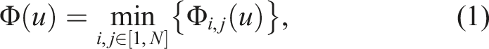
Sage Journals: Discover world-class research

Abstract

The capabilities of discovering new knowledge and updating the previously acquired one are crucial for deploying autonomous robots in unknown and changing environments. Spatial and objectness concepts are at the basis of several robotic functionalities and are part of the intuitive understanding of the physical world for us humans. In this paper, we propose a method, which we call Modelify, to incrementally map the environment at the level of objects in a consistent manner. We follow an approach where no prior knowledge of the environment is required. The only assumption we make is that objects in the environment are separated by concave boundaries. The approach works on an RGB-D camera stream, where object-like segments are extracted and stored in an incremental database. Segment description and matching are performed by exploiting 2D and 3D information, allowing to build a graph of all segments. Finally, a matching score guides a Markov clustering algorithm to merge segments, thus completing object representations. Our approach allows creating single (merged) instances of repeating objects, objects that were observed from different viewpoints, and objects that were observed in previous mapping sessions. Thanks to our matching and merging strategies this also works with only partially overlapping segments. We perform evaluations on indoor and outdoor datasets recorded with different RGB-D sensors and show the benefit of using a clustering method to form merge candidates and keypoints detected in both 2D and 3D. Our new method shows better results than previous approaches while being significantly faster. A newly recorded dataset and the source code are released with this publication.

Keywords

Incremental object database mapping object matching object merging depth data truncated signed distance field

1. Introduction

When the first robots appeared in industrial production lines, they have been considered as tools capable of performing only one specific task in an isolated environment. Because of the very strict requirements on accuracy, precision, and robustness, it has been very hard to claim safety and performance outside of these constrained conditions. However, recent advances in robotics are slowly changing the perspective and robots are gradually shifting towards solving more general tasks in less structured environments (Billard and Kragic 2019; Petersen et al., 2019).

Nevertheless, current systems are still not able to fully autonomously operate in real-world environments (Correll et al., 2016; Krotkov et al., 2017). Among the main challenges that still remain are general (unknown) environment understanding, robust mapping, and robot-environment interaction. Even though recent advances in certain areas such as instance segmentation, object detection, or localization, which solve parts of these challenges, perform very well for specific tasks, a system that is robust enough to operate in the real-world is still unseen.

In a scenario where a robot has to interact with the environment, these challenges become even more difficult. Such a task requires a robot not just to plan paths around objects but also to get close to them and, eventually, move certain objects by either pushing or grasping and placing them. For humans, identifying objects based on geometry and appearance is simple, as we typically have a very good notion of what constitutes an object, whereas for robots, we either need to learn or define such properties. In a general scenario, a robot does not know about the objects in the environment and, therefore, has no prior knowledge to what it might encounter. Furthermore, the robot needs to figure out which parts of the environment are relevant and it needs to be able to segment single objects such that it can interact with them. If the environment changes, either by the robot itself or another agent, the robot should still be able to localize and manipulate the objects. Because of these reasons, it is beneficial to have a map representation where parts of the environment which do not change over time with respect to each other (i.e., move jointly) are grouped together and form object-like structures. In addition to this, if such a part is observed multiple times, either through multiple sessions or repeating instances, this information should be used to infer unobserved parts of the objects.

This paper presents a system to address some of the aforementioned challenges. Specifically, without any prior knowledge about the objects in the scene, we maintain a 3D reconstruction of the environment, which is composed of object models stored in an incrementally generated database. Multiple instances or observations of an object are associated, fused, and finally used to complete the 3D models online. Since we rely on geometry to segment out the objects, the main assumption we make is that objects in the environment are separated by concave boundaries. Furthermore, our approach assumes that the sensor is well localized and that the scene is static.

This paper builds upon our previous work (Furrer et al., 2018), with the following new contributions:

• A novel merging strategy based on Truncated Signed Distance Field (TSDF) Root Mean Square Error (RMSE) and Markov clustering,

• Object matching and merging based on both 2D and 3D keypoints and descriptors,

• A time-synced and calibrated inertial RGB-D dataset with optimized poses,¹

• Evaluations of the system on multiple datasets,

• Source code of the system.²

2. Related work

Our system for incrementally creating 3D object models from RGB-D input data can be separated into three main components: segmentation and mapping; object description, matching and merging; and object clustering. We start by showing the image, depth, and scene segmentation literature, with a focus on instance segmentation, and how such techniques can be used to perform mapping on an object level. Then, we present the most relevant keypoint extraction, description, and matching techniques, both in 2D and 3D to find, align, and merge corresponding object segments. Finally, we discuss clustering methods that can be applied to determine which object segments should belong together, and show the most relevant systems that are similar to ours.

2.1. Segmentation and mapping

Image-based segmentation is a well-studied problem with a large number of works focusing on instance segmentation in RGB images. Traditional approaches try to group pixels with similar properties into superpixels and use optimization methods to refine their boundaries (Van Den Bergh et al., 2015). More recent, state-of-the-art methods use neural networks to predict object instances in images (Bolya et al., 2019; Chen et al., 2019; He et al., 2017; Huang et al., 2019). These mostly focus on finding instances of countable things, while leaving uncountable stuff unlabeled. To address this issue, a panoptic segmentation approach has been proposed by Kirillov et al. (2019). In addition to the RGB channels are also approaches that take advantage of the additional information provided by the depth channel of an RGB-D camera. Methods by Tateno et al. (2015) and Ückermann et al. (2013) segment regions in depth images based on surface normals and depth discontinuities, and Gupta et al. (2014) combine both RGB and depth image segmentation. Since robotic systems typically provide streams of images, the segmentation predictions can also be made on image sequences (Shelhamer et al., 2016).

In contrast to RGB and depth images, Dubé et al. (2019) proposed a method that first reconstructs the scene and then segments the object instances from the map. Furthermore, methods have been shown that segment the objects in the scene by tracking changes over time, either in live camera streams (Chen and Lu 2017), or in post-processing (Fehr et al., 2017). Surveys presenting methods for segmenting object instances in point clouds and meshes are provided by Nguyen and Le (2013) and Shamir (2006).

To obtain information about the segments in the map, that is, to recognize to which object they belong, segments can be matched to a database of known 3D models (Salas-Moreno et al., 2013; Tateno et al., 2016). Alternatively, a mapping framework (such as the one by Whelan et al. (2016)) can be used in combination with neural networks that provide per-frame predictions from a bounding-box object detector (Nakajima and Saito 2019; Sünderhauf et al., 2017; Zhang et al., 2018;) or semantic information together with the instance-segmentation (Grinvald et al., 2019; Hou et al., 2019; Mccormac et al., 2018; Runz et al., 2018). Because all of these approaches require prior knowledge about the objects to detect, either in the form of their corresponding 3D models or as extensive amounts of training samples, their applicability to unknown real-world environments is limited.

Our approach builds upon our previous work (Furrer et al., 2018), where we use a depth segmentation method, inspired by Ückermann et al. (2013), and integrated the obtained segments into a TSDF volumetric map, similar to Tateno et al. (2016). In contrast to our previous work, this approach uses a modified convexity measure in the segmentation.

2.2. Segment matching and merging

To complete the object models, a matching and merging step is required. Traditional approaches use distinctive points, either in 2D, based on image gradients (Lowe 2004), or in 3D, using surface normal gradients (Sipiran and Bustos 2011; Zhong 2009). Descriptors are computed using their local neighborhood (Rusu et al., 2009; Tombari et al., 2010). A review of methods that use local photometric features in 2D images was presented by Mikolajczyk and Schmid (2005), and in 3D by Guo et al. (2014). Recently, self-supervised methods (DeTone et al., 2018) have shown very promising results for feature prediction and description.

After obtaining and describing the features for each segment, matching is performed. This can be done by using a kd-tree structure of the descriptor space (Muja and Lowe 2014), or by clustering descriptors in the descriptor space and using these clusters as higher-level features (Sivic et al., 2005). Among other approaches, one can use large scale global matching, as presented by Liu et al. (2017). From a set of corresponding descriptors, an alignment between the segments can be obtained using sampling based methods such as Random Sample Consensus (RANSAC) (Fischler and Bolles 1981), least-squares fitting on the two 3D point clouds (Arun et al., 1987), or with optimization-based global registration (Zhou et al., 2016). These initial transformation estimations can be refined using Iterative Closest Point (ICP) (Aldoma et al., 2012; Besl and McKay 1992) approaches. Recent work by Avetisyan et al. (2019) used learning methods to find alignments of CAD models to reconstructed scenes.

In contrast to traditional approaches that perform feature matching and registration, recent learning-based methods can detect objects in 2D images (He et al., 2016; Lin et al., 2017), RGB-D frames (Schwarz et al., 2018; Qi et al., 2018) or in 3D point clouds (Shi et al., 2019; Zhou and Tuzel 2018). As we do not want to be biased by the training data provided to the supervised methods, we rely on traditional methods for feature extraction and registration.

Previously (Furrer et al., 2018), we used 3D keypoint detectors and descriptors to obtain features in point clouds. Then the Fast Library for Approximate Nearest Neighbors (FLANN) (Muja and Lowe 2014), RANSAC, and ICP, were used to obtain feature matches, and the alignment of the segments. Our current approach, in addition to 3D features, also uses 2D features obtained from RGB images. We use the depth information to project 2D features into 3D, and integrate them into a volumetric 3D feature map based on Voxblox (Oleynikova et al., 2017), similar to our segmentation map. Finally, a matching step is performed for both 2D and 3D features and the transformation which provides the better merging measure is retained.

2.3. Clustering

Our goal is to create object models from an unknown number of geometric segments, extracted from a segmentation map. A naive approach is to try all combinations of matching segments (Furrer et al., 2018). A more scalable way is to merge only certain disjoint sets of segments. This can, for instance, be achieved by forming clusters in a graph with pairwise segment matching scores as edge weights. Clustering methods, where the number of clusters does not have to be specified, are shown by Dongen (2000) and Frey and Dueck (2007). Affinity propagation (Frey and Dueck 2007) works by computing similarities among all segments (vertices) in a graph. Markov Clustering (Dongen 2000) and Repeated Random Walks (Macropol et al., 2009) on the other hand, try to separate clusters at locations where there are only few or week connections. Here, we have selected Markov Clustering to be integrated in our system.

2.4. Systems

Systems like (Ekvall et al., 2007; Nakajima et al., 2018; Tateno et al., 2016) can map the environment on an object level using known objects from a database. However, these approaches cannot update the existing models with new observations. The closest works compared to ours are the ones that extract 3D object models in changing environments. In this regard, change detection has been applied on a frame to map basis using RGB-D data (Herbst et al., 2014) or a scene to scene comparison, by comparing TSDF grids (Fehr et al., 2017) of different recordings and by extracting point clusters, as in Meta-rooms (Ambruş et al., 2014; Ambrus et al., 2017). To the best of our knowledge, no prior work (except for our previous approach (Furrer et al., 2018)) has demonstrated the ability to incrementally extract and update object models.

3. Method

In our method, we tackle the problem of building segmented 3D maps of the environment and simultaneously constructing 3D models of the objects present in the scene. We first integrate segments extracted from RGB-D sensor data into a volumetric map of the scene that contains the geometry and a label per segment. Once these segments are no longer in the current camera frustum, we insert them into a database. We store the TSDF grids representing the segments, together with keypoints and descriptors, and their poses in the map. Keypoints and descriptors are obtained from 2D (RGB images), and 3D data (extracted geometry from the segmentation map). In the database, we try to match and align these new segments with segments inserted previously. If we get a successful pairwise match, we perform an evaluation step where we check if the updated, fused object model fits the scene geometry at the pose of each observed object instance. Based on these scene evaluations, we compute a matching score and use a graph-based clustering approach to allow merging of multiple segments (see Figure 1).

Figure 1.

The Modelify pipeline. Depth images are used to segment the current frame into geometric segments which are integrated into a segmentation map. 2D features are extracted from the RGB images and integrated with the depth information into a feature map. Single segments from the segmentation map are described and matched to previously observed segments. With the error score from the verification steps as edge weights and the segments as nodes, we create a graph and a clustering algorithm is used to propose merge candidates which undergo another scene verification step.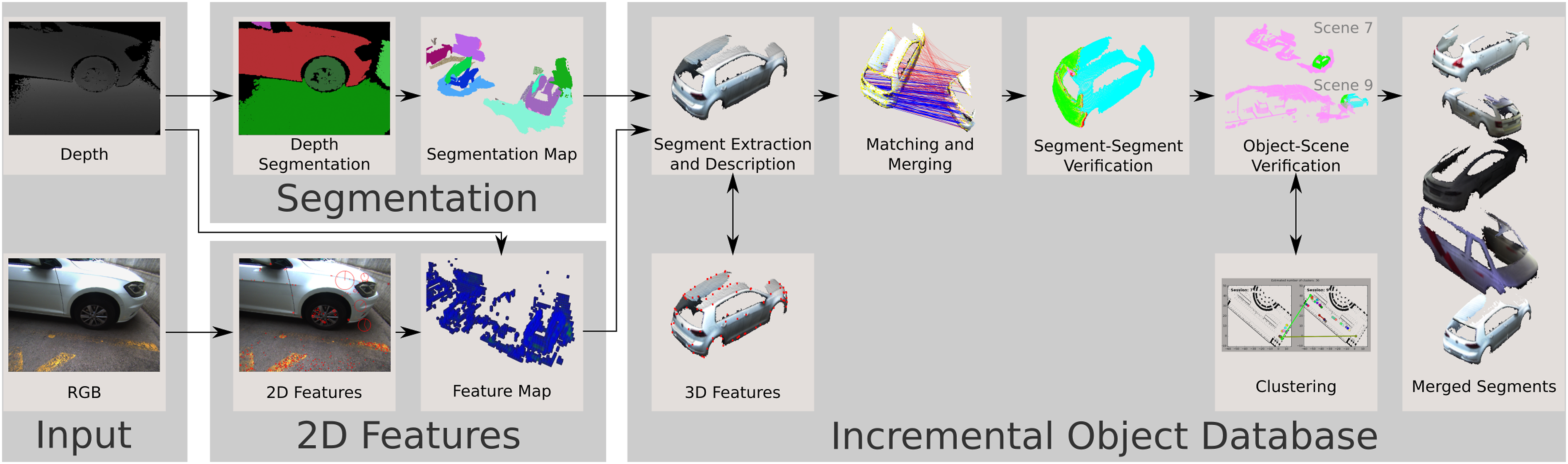

Every new run of our pipeline is considered a new session and during each session a local map is created. This map, together with the geometric object segments, is stored in the database. The map is required to evaluate merge candidates at all occurrences in all the scenes where individual segments, that constitute the merge candidate, appear.

3.1. Segmentation

As we did not want to rely on a learning-based method that is biased by its training data, the depth segmentation approach we use exploits only geometric properties to extract individual segments. Furthermore, based on the assumption that concave regions separate real-world objects, we decided to use a local convexity measure as one of our main segmentation criteria. Since we observe the environment discretely, this assumption does not always hold, as it depends on how densely we sample the geometry, that is, resolution of the sensor and how far from the surface we are. Nevertheless, we found it to be a very effective geometric measure, together with the depth discontinuity, that allows us to extract most of the objects from the scene.

In our approach, we first compute normals based on depth distribution in a local pixel neighborhood of the depth image. We then use these normals to obtain the local convexity measure for each pixel and use this information to obtain a map of convex regions. Next, edges that exhibit strong discontinuities in depth are detected. Finally, convexity and depth discontinuity maps are combined to obtain closed regions for which we then assign segment labels. These labels are not consistent between different frames. From each of these regions, a pointcloud is generated which then constitutes our labeled 3D segment.

Before computing the normals, we optionally inpaint the depth image to fill small areas with missing data and obtain more continuous areas of valid depth values. The necessity of this step depends on the output data of the sensor. For example, a depth image from the Tango sensor has circular artefacts which can be observed in Figure 2 in the top left image.

Figure 2.

The steps of the depth segmentation illustrated on the tango dataset. Top row, left to right: raw depth image, RGB image, normal map. Bottom row left to right: discontinuity map, convexity map, output segmented depth image.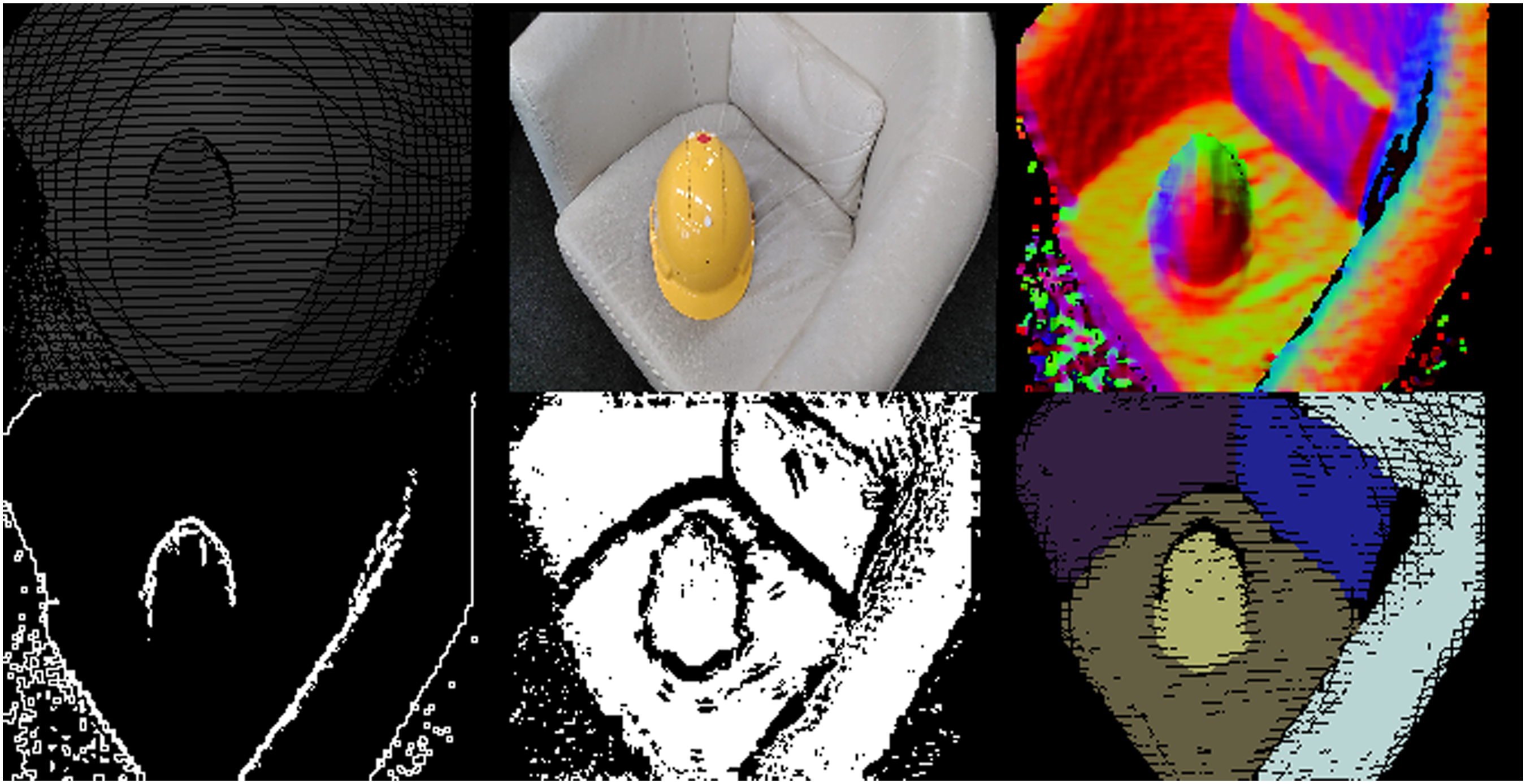

Using the inpainted (or original) depth image, we compute the normal estimates for each pixel in the image. To obtain these, we follow the Principal Component Analysis (PCA) method from Rusu (2009). First, a covariance matrix is computed from a local neighborhood for each pixel in the depth image. Then, we obtain eigenvalues and eigenvectors from this matrix. Finally, the eigenvector corresponding to the lowest eigenvalue is selected as the normal estimate for that pixel. This vector geometrically represents the normal of a best-fitting plane in that local neighborhood. 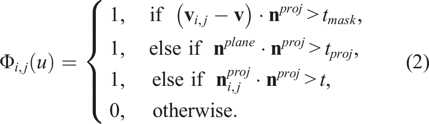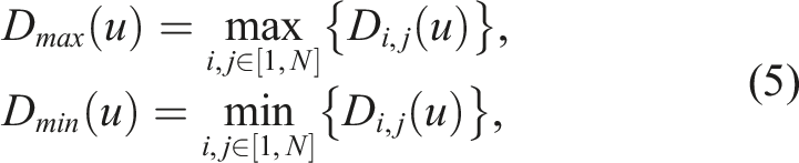Once we compute these estimates, $n$ , for each pixel, we obtain a normal map.

The convexity measure, in contrast to our previous approach (Furrer et al., 2018), is obtained by taking the minimum value of all convexities in a given kernel of size $N$ by $N$

Φ (u) = \min_{i, j \in [1, N]} {Φ_{i, j} (u)},

(1)

where

u

is the kernel anchor (center point of the kernel) pixel location in the image and

Φ_{i, j} (u)

is the convexity of

u

using the

(i, j)

coordinate of the kernel, and is equal to

Φ_{i, j} (u) = {\begin{array}{c} 1, & if (v_{i, j} - v) \cdot n^{p r o j} > t_{m a s k}, \\ 1, & else if n^{p l a n e} \cdot n^{p r o j} > t_{p r o j}, \\ 1, & else if n_{i, j}^{p r o j} \cdot n^{p r o j} > t, \\ 0, & otherwise . \end{array}

(2)

The point locations in 3D, $v$ and $v_{i, j}$ at pixel locations $u$ and $u_{i, j}$ , respectively, are used to calculate the normal of the plane that goes through these points and that contains the sensor’s $z$ -axis, that is, the plane is perpendicular to the image plane

n^{p l a n e} = \frac{z \times (v_{i, j} - v)}{| z \times (v_{i, j} - v) |} .

(3)

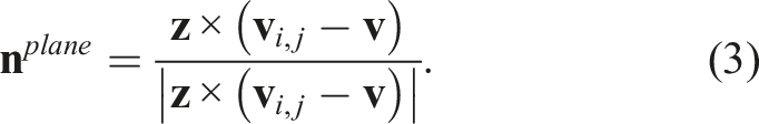
The normalized plane normal $n^{p l a n e}$ and the normal $n$ , obtained in the previous step, at pixel location $u$ are then used to obtain the normal projected into the previously defined plane

n^{p r o j} = \frac{n - (n \cdot n^{p l a n e}) \cdot n^{p l a n e}}{| n - (n \cdot n^{p l a n e}) \cdot n^{p l a n e} |} .

(4)

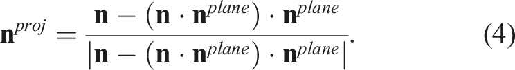
All the normals $n^{p r o j}$ , $n_{i, j}^{p r o j}$ , and $n$ are functions of pixel location $u$ and/or current kernel indices $i, j$ , however, we have omitted these in the equations to simplify the notation. The sensor’s $z$ -axis vector is constant and equal to $[0, 0, 1]$ .

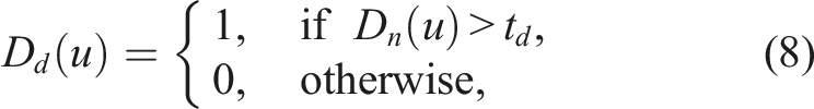
With the projected normals $n^{p r o j}$ and $n_{i, j}^{p r o j}$ at locations $u$ and $u_{i, j}$ , and specified thresholds $t_{m a s k}$ , $t_{p r o j}$ , and $t$ , we can obtain the convexity measure for a specific kernel location $Φ_{i, j} (u)$ . Once the convexity measure is calculated at all kernel locations, the minimum is taken as the resulting convexity for location $u$ , $Φ (u)$ .

If the threshold $t_{m a s k}$ is set to 0, the first condition in equation (2) defines the convex regions as the ones where the vector from the anchor to the current kernel point is oriented in the same direction as the projected normal at the anchor point, that is, the dot product is larger than 0. By modifying the threshold $t_{m a s k}$ , we can adjust the number of points that are considered to be in a convex neighborhood. For example, even vectors that do not point in the same direction can be considered convex if we set the threshold $t_{m a s k} < 0$ . The second condition in equation (2) discards directions for which the point normal $n$ is almost perpendicular to the normal of the projection plane $n^{p l a n e}$ , since such convexity measurements are unreliable, that is, a small change in the normal direction drastically changes the projection. The last condition in equation (2) provides a measure of convexity for the remaining points and $t$ specifies a threshold above which the points will be considered convex.

The main improvements to our previous approach are twofold. Firstly, we are using normals projected into planes defined by the anchor point, the point at the current kernel position and the sensor’s $z$ -axis, instead of actual 3D normals. This allows us to only consider the convexity measure along desired directions, defined by the kernel points, thus improving the estimate. And secondly, we have added an additional filtering condition, the second condition in equation (2), which allows us to reject directions where the convexity measure might be unreliable, resulting in a smoother convexity map. The resulting segmentation using the new convexity measure can be observed in Figure 2. An image comparing it to our previous approach is shown in Figure 3. In the previous approach, we inpainted the depth image and used it for the rest of the approach, while in the new approach, the inpainted image is only used to compute the normals. That is the reason why the old segmentation output looks denser.

Figure 3.

Comparison between the output of our old segmentation (Furrer et al., 2018), on the left, and the new approach, on the right, which uses modified convexity measure. As it can be seen in the right image, the helmet and the back cushion are segmented from the seat cushion, while this is not the case in the left one.

In addition to the convexity measure, we use the depth discontinuity as a cue for segmentation. To obtain it, we follow the method by Singh et al. (2014). We first compute the $D_{\max}$ and $D_{\min}$ images, from the original depth image $D$ , for each pixel location $u$

\begin{array}{l} D_{\max} (u) = \max_{i, j \in [1, N]} {D_{i, j} (u)}, \\ D_{\min} (u) = \min_{i, j \in [1, N]} {D_{i, j} (u)}, \end{array}

(5)

where

N

N

is the kernel size. Then, we find the largest local depth change in the neighborhood

D_{c h} (u) = \max {D_{\max} (u) - D (u), D (u) - D_{\min} (u)} .

(6)

Finally, we normalize the largest depth change image with the original depth value

D_{n} (u) = D_{c h} (u) / D (u),

(7)

and then apply a threshold

t_{d}

to it

D_{d} (u) = {\begin{array}{c} 1, & if D_{n} (u) > t_{d}, \\ 0, & otherwise, \end{array}

(8)

to obtain the depth discontinuity map.

In a final step, the inverted convexity and depth discontinuity maps are combined to obtain an image which contains segment boundaries, see Figure 2. These boundaries are extracted as contours, and all the pixels that fall within a single contour are labeled with the same label, representing the same segment.

Even though we use a geometric segmentation approach, our system is flexible and any other segmentation that provides a set of segments (as point clouds) can be used. Furthermore, even a pre-trained network for semantic instance segmentation, as we have shown in (Grinvald et al., 2019), can be used to obtain semantically meaningful segments.

3.2. Segmentation and feature map

In order to have a consistent segmentation over multiple frames, we require a mapping framework that is able to recognize which newly extracted segments belong to which previously extracted segments. To do this, we have implemented our own segmentation map, which is based on TSDF. Such a volumetric framework allows us to more easily associate data (all points that fall into the same voxel are considered to be the same), is very fast at integrating data, provides a very good quality of the reconstruction, and can map free-space, which is very useful for evaluating the quality of an object alignment, as shown in the next subsection.

The segments from the depth segmentation step are integrated into the volumetric map. As described in detail in our previous work (Furrer et al., 2018; Grinvald et al., 2019), we assign each segment that we integrate a label which is consistent with the labels in the map. For each voxel in the map, we keep the history of labels that appeared at that location with the corresponding frequency of observations. In our approach, we assume that the scene is static such that we can properly reconstruct it. The result of the integration is a segmentation map, of which an example is shown in Figure 4(b). When a segment gets extracted, the label that has the most observations is assigned to it.

Figure 4.

The feature and segmentation maps of a single car scene, (a) and (b) are observed from the same view-point.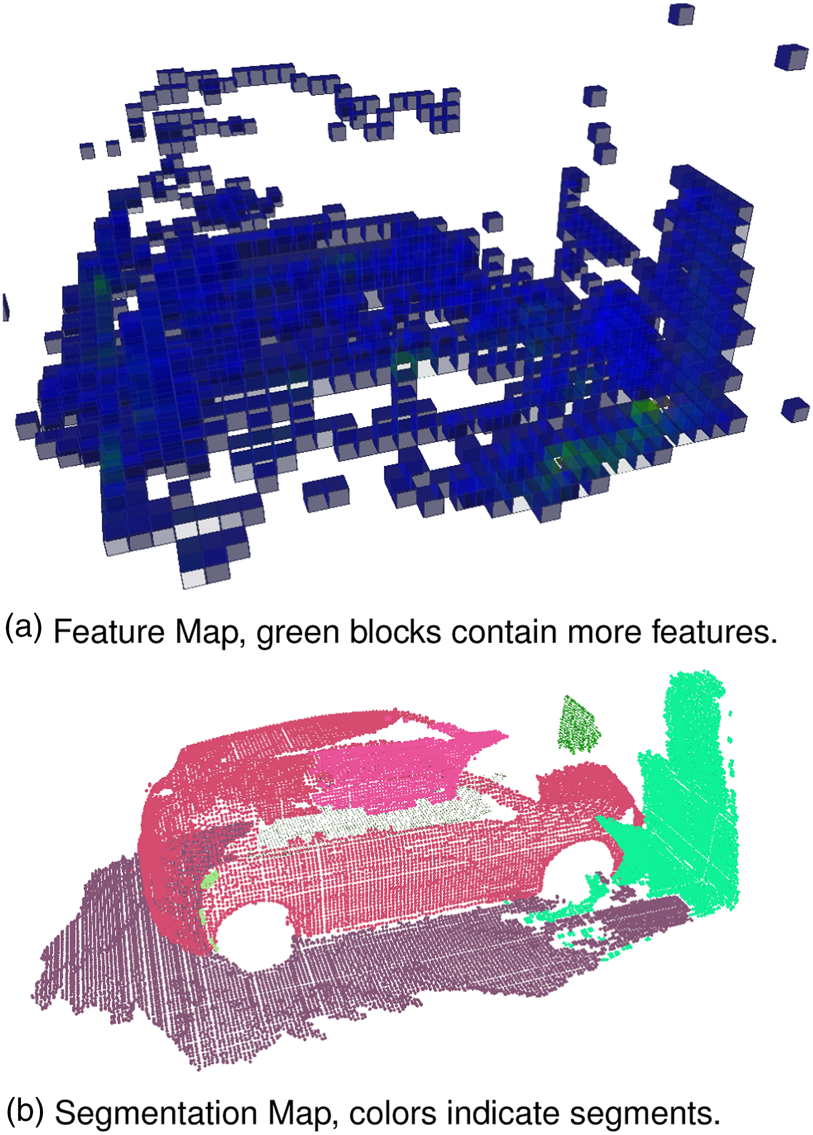

Along with the segmentation map, we build a feature map where we integrate 2D features, extracted from RGB images, at their 3D location in a map, Figure 4(a). 2D features represent salient points in RGB image whose 3D location is obtained from the registered depth image and the current camera pose. We use a volumetric representation for our scene creation that is based on Voxblox (Oleynikova et al., 2017). The volume is split up into blocks that contain multiple voxels addressed using unique hashes (Niessner et al., 2013). In addition to the voxel blocks, we created a new block type that only contains features. Therefore, inserting new features into the feature map is very efficient as it requires only a single lookup in the hash map to obtain the proper block index. Each feature block contains a vector of all the features that were observed in this volume. Each feature represents the keypoint’s location in 3D, its response, and its descriptor. Additionally, before inserting any new feature, an online brute force matching to all the features already contained in the block is performed. If the new feature is too similar to any of the features already in the block, it is discarded. The feature map is compatible with any type of 2D features. In our experiments, we use SIFT (Lowe 2004) because it provides very descriptive features and we can afford to compute it since the bottleneck of our pipeline is depth segmentation, which runs at approximately $3 H z$ .

Since the underlying structure of the blocks in the segmentation and the feature map is identical, the same hashing function can be used to access the same locations in space. Therefore, once we extract a segment, the same volume in space is extracted from both maps. This volume contains a TSDF grid, a segment label, and a grid with feature blocks containing 2D features in 3D which is then transferred to the incremental database, Figure 1. The features in each block are sorted by their keypoint response and limited by a parameter for the maximum number of extracted features per block.

3.3. Incremental object database

Once a segment from the segmentation map is received by the database, the first step is to check if it is planar. This information is required later on to decide if an ICP registration step should be performed. Next, we find keypoints and compute descriptors. If we fail to find 2D and 3D keypoints, we mark the segment as unmergeable, as we are unable to match it with other segments. Before we insert the described segment into the database, we match it with all the segments that are already in the database to find matching segments. Afterwards, we evaluate all the matching segments and perform a graph-based Markov clustering to obtain candidate merges. These merge candidates are reprojected at each observed location of the segments present in the cluster and checked for consistency in all the scenes. We accept merges that are consistent with the scene at all their occurrences.

3.3.1. Segment description

As described in Section 3.2, segments received by the database contain two grids, a TSDF and a feature grid. We extract a mesh from the TSDF volume using the Marching Cubes algorithm (Lorensen and Cline 1987). Afterwards, we convert the mesh vertices to a pointcloud with vertex normals and remove duplicate points. We use RANSAC-based plane fitting to check if the segment is planar. We allow to merge planar segments in the database only with a disabled ICP registration to avoid unconstrained alignments. During registration of planar segments (using ICP with point-to-plane error metric), there are infinitely many solutions with an optimal error, that is, any transformation for which surfaces just slide along the plane results in the same (or a similar) error. We compute the cloud resolution to scale the parameters of the used Harris (Sipiran and Bustos 2011) and Intrinsic Shape Signatures (ISS) (Zhong 2009) 3D keypoint detectors. Finally, Fast Point Feature Histograms (FPFH) (Rusu et al., 2009) descriptors are computed for the detected 3D keypoints.

From the feature layer, we extract the 2D features, as 3D points. Since these points are no longer on the surface of the segment, due to TSDF averaging and pose inaccuracies, for each 2D feature, we find the nearest neighbor (within a distance threshold) in the segment pointcloud and insert it into a keypoint cloud of the 2D keypoints. Each of these points in the keypoint cloud also has an accompanying 2D descriptor and keypoint response. Once all the 2D features are assigned to a point in the segment point cloud, we perform a non-max suppression step, to only keep a certain amount of keypoints, the ones with the highest keypoint response, within a certain radius. This way, we reduce and bound the total amount of 2D keypoints and only keep the best ones. We depict one segment with the associated 2D and 3D keypoints in Figure 5

Figure 5.

A textured car model with 2D keypoints in red and 3D keypoints in yellow. The right half of the car is colored by vertex normals.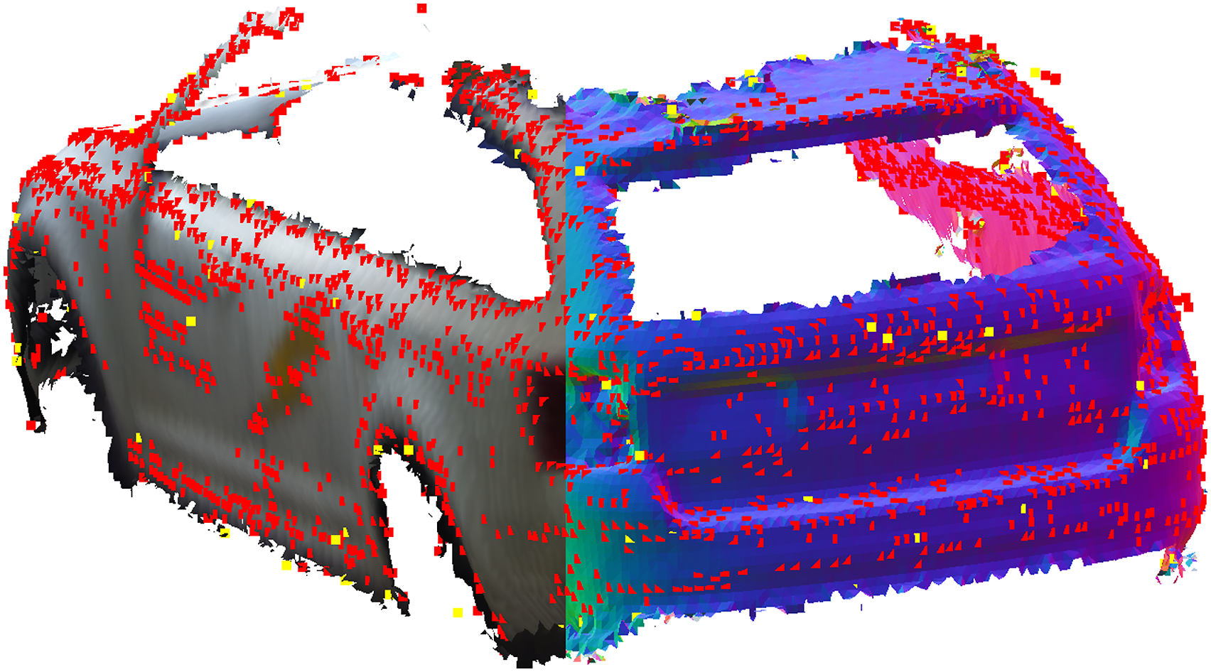

3.3.2. Matching, alignment, and evaluation

In the matching step, we first find initial 2D and 3D feature correspondences, using FLANN, by Muja and Lowe (2014), for the 3D features, and brute force matching with L2 norm for the 2D features, illustrated in Figure 6. Then we perform a RANSAC step to find initial alignments for both the 2D and 3D feature matches, and refine these alignments using a point-to-plane ICP registration (Chen and Medioni 1991).

Figure 6.

Matching two car segments using FLANN and FPFH (a) and SIFT (b) descriptors of Harris3D (a) and SIFT (b) keypoints (yellow), with discarded matches (red) and accepted matches (blue).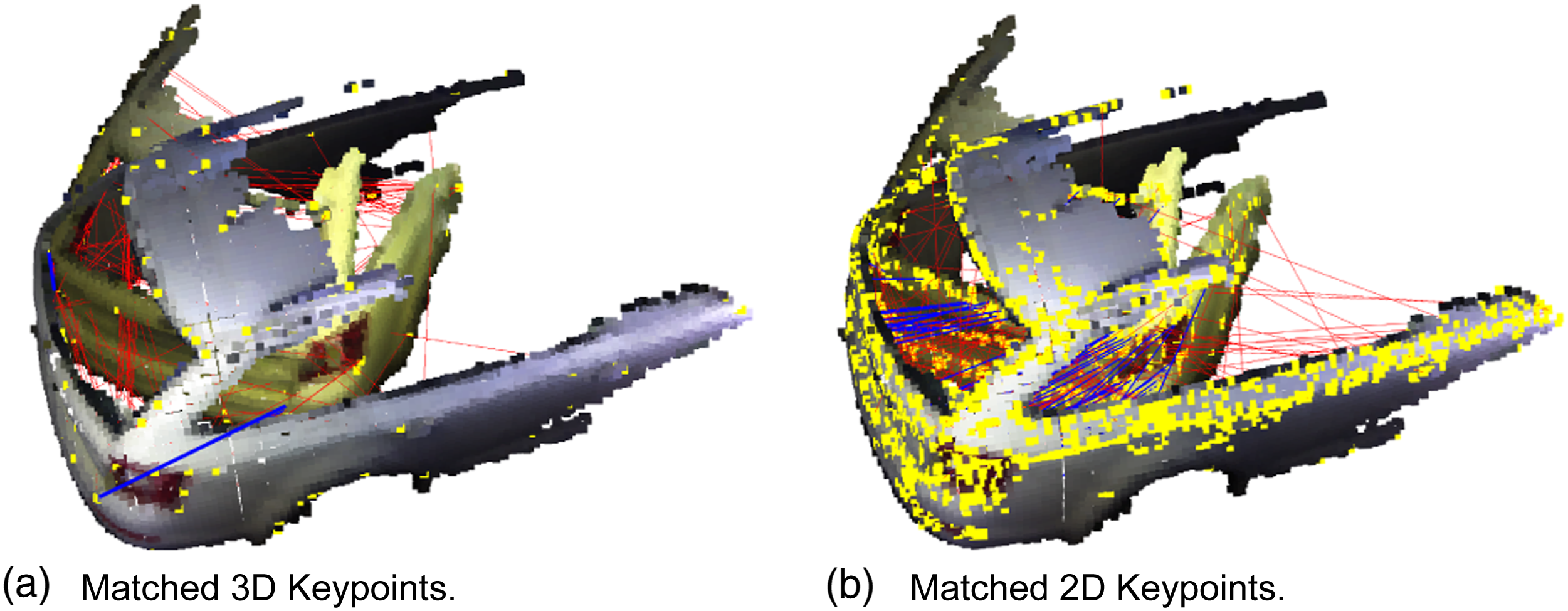

To generate instances of these merge candidates, we align the segments with the estimated transformations, from the RANSAC and ICP steps, with both 2D and 3D alignments, shown in Figure 7(a). We use trilinear interpolation to align the TSDF grid of the transformed segment. By comparing the TSDF values of the overlapping voxels from the two aligned segments, we can compute a RMSE denoted as the segment-segment error

e_{T S D F} = \frac{1}{| O |} \sum_{\forall k \in O} \sqrt{{(t_{j, k} - t_{i, k}^{'})}^{2}},

(9)

where

t_{j}

and

t_{(i)}'

are the TSDF grids of segment

j

and segment

i

aligned to the

j

segment, and

O

is the set of indices of the overlapping voxels. An example of a TSDF value comparison is depicted in Figure 7(b). In addition to this average error value

e_{T S D F}

, we noticed that properly matching segments have a large portion of the overlapping voxels at low errors, but sometimes suffer from larger errors at the boundaries of the segments. This often resulted in an average error that was higher than the one of not matching segments that just happened to be nicely aligned in the ICP step. Hence, we bin the error values of the segment-segment evaluation into a histogram

H

, with equally sized bins. The values of bins

h_{i}

are the counts of values in the bin range

h_{i} = \sum_{k \in O} {\begin{array}{c} 1 & if e_{T S D F, k} \in [i \cdot h_{w}, (i + 1) \cdot h_{w}), \\ 0 & otherwise, \end{array}

(10)

where

h_{w}

is the bin width. In our approach, it is sufficient to ensure that the first bin captures a higher portion of the error values than a threshold

t_{1 s t b i n}

. If both 2D and 3D alignment proposal pass these verification steps, we discard the proposal with the higher segment-segment error

e_{T S D F}

Figure 7.

The two matched segments from Figure 6 are aligned using ICP (a) and result in a per voxel TSDF error in (b), where green indicates a low error and red a large error.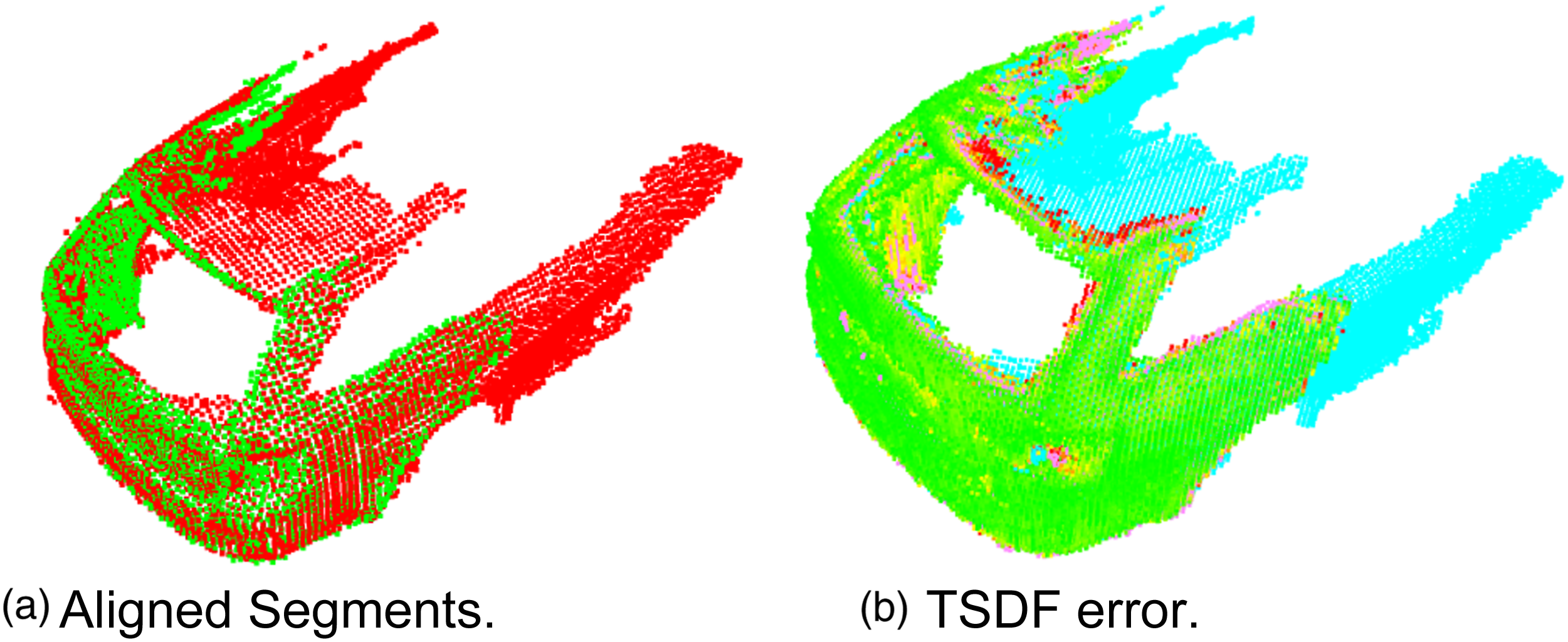

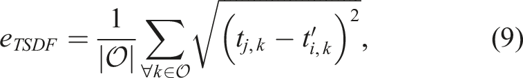
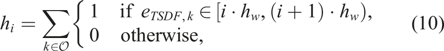
As an additional step, we check if the resulting object model from merging segments conforms with the reconstructed scene(s) by reprojecting the model to all the locations where the single segments were observed. This check again gives us an RMSE, which we denote as object-scene error $e_{s c e n e}$ , computed the same way as $e_{T S D F}$ just replacing the individual segments with the merged segment and the scene, respectively. This value is then used to compute a matching score for the clustering step.

Free-space information, which is also stored in the TSDF representation, is very valuable when performing this check. In case we end up with an incorrect merge candidate, once it is reprojected into the scene, at the location of each segment, it is likely that it will result in a high object-scene error since it will occupy the space that should otherwise be free-space. This notion of free-space is therefore crucial for evaluation of the object models that we create.

3.3.3. Clustering

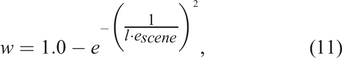
In this step, we obtain clusters based on the previously computed matching scores. We do this by forming a graph, where each node represents a geometric segment. Edges are inserted into the graph if matching, merging, and evaluations among two segments were successful. For the edge weight $w$ , we use the object-scene error $e_{s c e n e}$ in a normalized form

w = 1.0 - e^{- {(\frac{1}{l \cdot e_{s c e n e}})}^{2}},

(11)

where

l

is a parameter that indicates the width of the function and can be set based on the object-scene RMSE threshold. We chose to use Markov clustering (Dongen 2000) to form clusters for two reasons, it allows to form an unknown number of clusters in a graph and it allows to have sparse graphs and ensures that no vertices are connected that do not have an actual connection. An example outcome of our clustering is shown in Figure 8. Each cluster, a merge proposal, is merged and again verified in the scene. If a scene verification fails, we remove all edges between the newest segment in the graph and the failing cluster vertices. In order to not duplicate checks, we do scene evaluations only for clusters with at least three segments (as we already did the scene verification for segment pairs) and we keep a list of already performed scene evaluations. We redo an already existing scene evaluation only if it contains the latest segment.

Figure 8.

Clusters formed while evaluating the three sessions of the tango dataset. The vertex colors indicate to which cluster the segments belong and the edges indicate that there was a match between two segments. The line width indicates the matching score.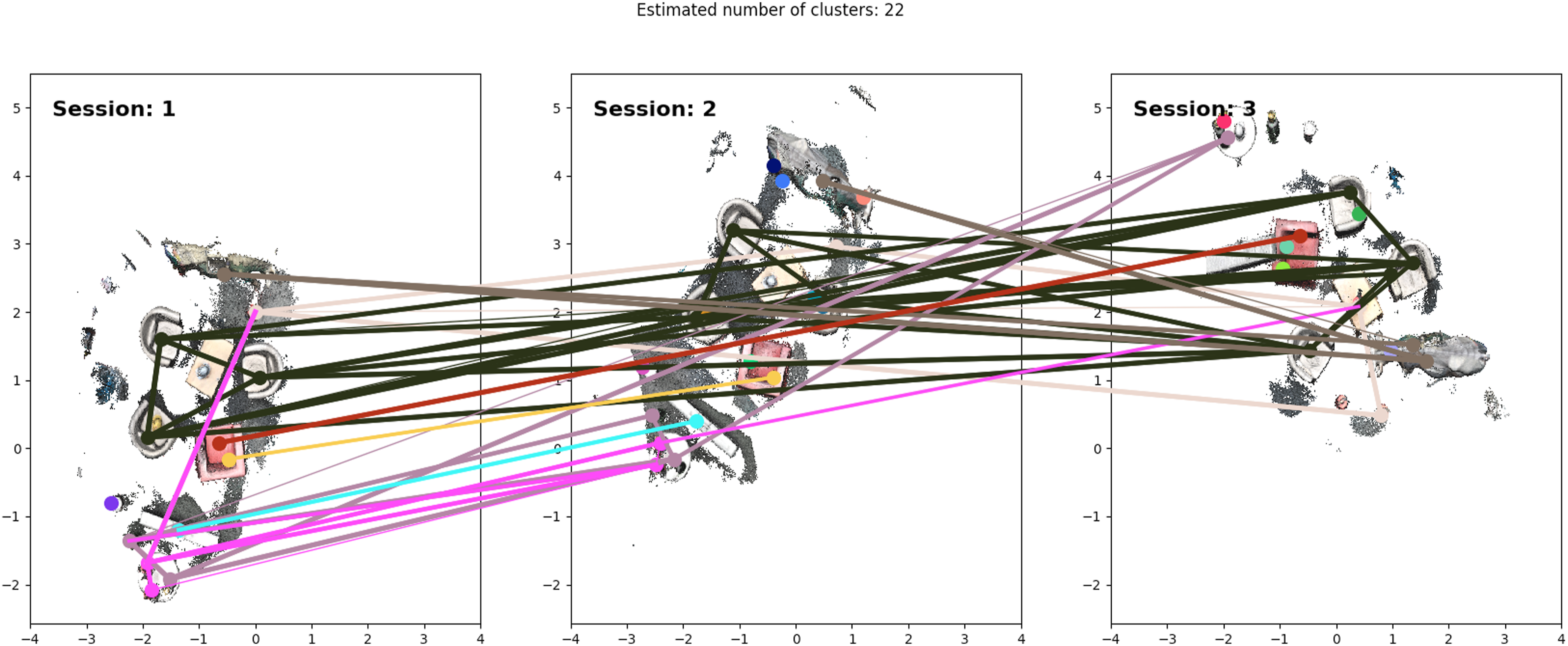

3.3.4. End-of-session merging

With the advantage that the clustering approach gives us clusters, as segments change in the scene, it has the drawback that sometimes it also separates segments belonging to one object in multiple clusters. To overcome this limitation, we can perform a final merging step after a session is terminated, among all the clusters (including clusters of size 1).

The end-of-session merging is an iterative process that first tries to find merges between all single unmerged segments. Then all the merged segments are matched against each other. This step is followed by an iteration where all single unmerged segments are matched to the merged ones. Finally, another iteration of matching between merged segments is performed. If there are any matches that pass the same conditions as explained before, they are merged and added to the database. In contrast to the clustering-based merging strategy where we only match segment pairs, the end-of-session merging can perform matching and merging between merged segments. This has the advantage to work with more complete data and can merge segments that otherwise would not match.

4. Results

For the evaluations, we use a set of publicly available datasets, released in previous publications, in addition to a newly recorded dataset with a custom RGB-D-I sensor. We show both quantitative and qualitative results for map creation and segment merging. As to the best of our knowledge, there is no other system that merges object instances and uses them to complete scenes. Hence, we only compare with our previous method, both in terms of quality and timing.

4.1. Datasets

We show results on an indoor dataset recorded with a Google Tango device, which also served as the main evaluation dataset in our previous work (Furrer et al., 2018). In addition to this, we show that this method can be used to automatically create 3D models of household objects in cluttered box scenes (Novkovic et al., 2019). Finally, we collected a new RGB-D-I (using a color and depth camera, and an Inertial Measurement Unit (IMU)) dataset that contains sequences in a parking garage. We show that the method is applicable also for such large scenes and that we can extract and merge segments even in outdoor environments with changing light conditions.

4.1.1. Tango

This dataset contains indoor scenes with two kinds of chairs, two small tables, a set of fire extinguishers and gas bottles, two kinds of helmets, a cylindrical and a box-shaped container, as well as an artistic cow. The three reconstructed session scenes are displayed in Figure 9. Sessions 1 and 2 are two runs on the same scene, whereas the objects are rearranged in Session 3. The camera poses are optimized poses obtained by the tango mapping framework.

Figure 9.

Qualitative results of the three sessions of the tango dataset (Session 1 (left), Session 2 (middle), Session 3 (right)). The rows show the scene reconstructions (top row), the ground truth annotated segments (second row), the output of the segmentation map (third row), and the completed reconstructed scenes (bottom row), where blue indicates that data is in the recorded dataset and red shows completed objects stemming from the merged segments.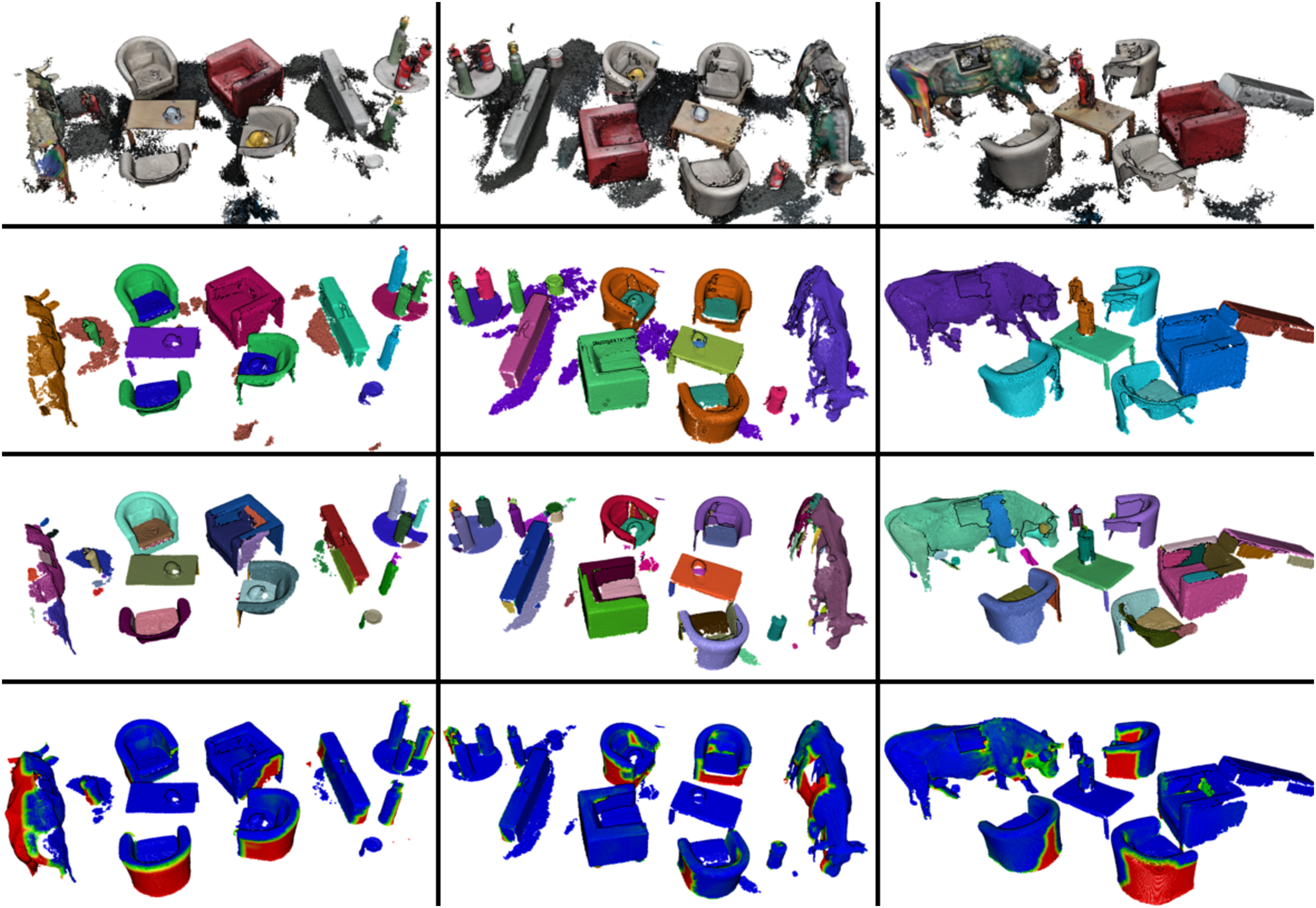

4.1.2. CLUBS

As presented in a previous publication (Novkovic et al., 2019), this dataset contains RGB-D images of household objects captured with cameras attached to a robotic end-effector. There are two different kinds of scenes: cluttered warehouse distribution box scenes containing up to 40 objects, and object scenes where an isolated object is placed on a table. In box scenes, only a limited portion of each object is visible, whereas objects are visible as a whole, except for the bottom, in object scenes. To also capture the bottom of the object, the dataset contains two object scenes per object, where in the second scan, the objects are rotated upside down. For the purpose of this work, we optimized the camera poses of box scenes using a bundle adjustment approach that includes 2D feature matches and a point-to-plane ICP error metric.

There are 85 object and 25 box scene configurations in the CLUBS dataset (see Novkovic et al. (2019) for more details). Box scenes were recorded in multiple iterations such that in the first iteration all the objects would be placed in the box. Then the box would be scanned (from nine different poses), one object would be taken out and then the next iteration would start. This would be repeated until there would be no objects left in the box, more specifically for 30 or 40 iterations depending on the box. For object scenes, 19 different poses were used during scanning.

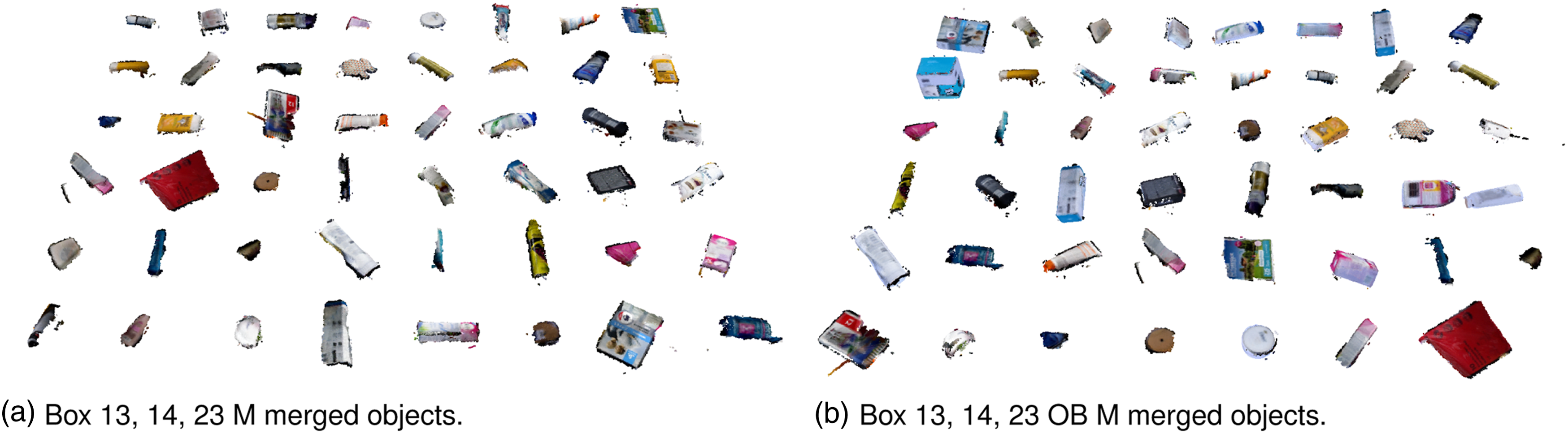
From this dataset, we selected four iterations from boxes 13 and 14, and 6 iterations from box 23. These were selected because they contain repeated instances of objects, their configurations of the objects in the box are random, and a large number of objects can be found in more than one of the three boxes. Additionally, we selected 20 different objects that were contained and often repeating inside of the three boxes, and used their 40 object scenes (each object is scanned twice) to generate object models. We used the depth data from the PrimeSense Carmine 1.09 sensor and the color images from the RealSense D435 for the box scenes, and depth and color from the RealSense D435 for the object scenes. Different depth sensors were used to show that we can merge objects even if they do not arrive from the same sensor (the PrimeSense Carmine 1.09 is a structured light sensor with relatively little noise, while the RealSense D435 uses an active stereo approach to obtain the depth image at a higher resolution but also noisier). The RealSense D435 RGB color image is used since it provides the highest quality RGB image compared to the other sensors and therefore consequently the best 2D features. To obtain cleaner depth images, the box in the background is subtracted from each depth image for the box scenes. We did this to reduce the total amount of segments we have, such that the data is faster to annotate with the ground truth, and that the results are more easily traceable and easier to evaluate. In practice, this step should be easy to do since for most of the applications in a typical warehouse robotic setting, where such box scenes are often encountered, it can be assumed that locations of scanned boxes are precisely known. We apply our approach, as depicted in Figure 10, to incrementally form a dataset of the contained objects.

Figure 10.

Our system is able to build object model database incrementally from RGB-D sensor streams. Here, we illustrate how the approach generates 3D models of household objects from distribution box scans, taken at different places around the box by a camera attached to a robot arm’s end-effector (Novkovic et al., 2019). As we match and merge new segments with models already in the database, we improve the models over time and can even complete unobserved parts of scenes. From top to bottom, different box scenes are evaluated. First the same box and same session evaluated at single snapshots (different frames). Then at different fill levels (different session), and eventually also different boxes. Highlighted in the first two rows is one repeating object, visible in the same frame, which is merged in the database (second column) and can be used to complete the reconstructed scene (third column). More segments are added to the database, while repeating objects get merged. Columns 3–6 show scene completions of the different times with the objects available at these time instances. The last row is a scene with the isolated object. Using such scenes that contain entire objects, the box scenes can be completed even more, best visible in the bottom row. Red color indicates parts of the objects that are completed using information from the other sessions.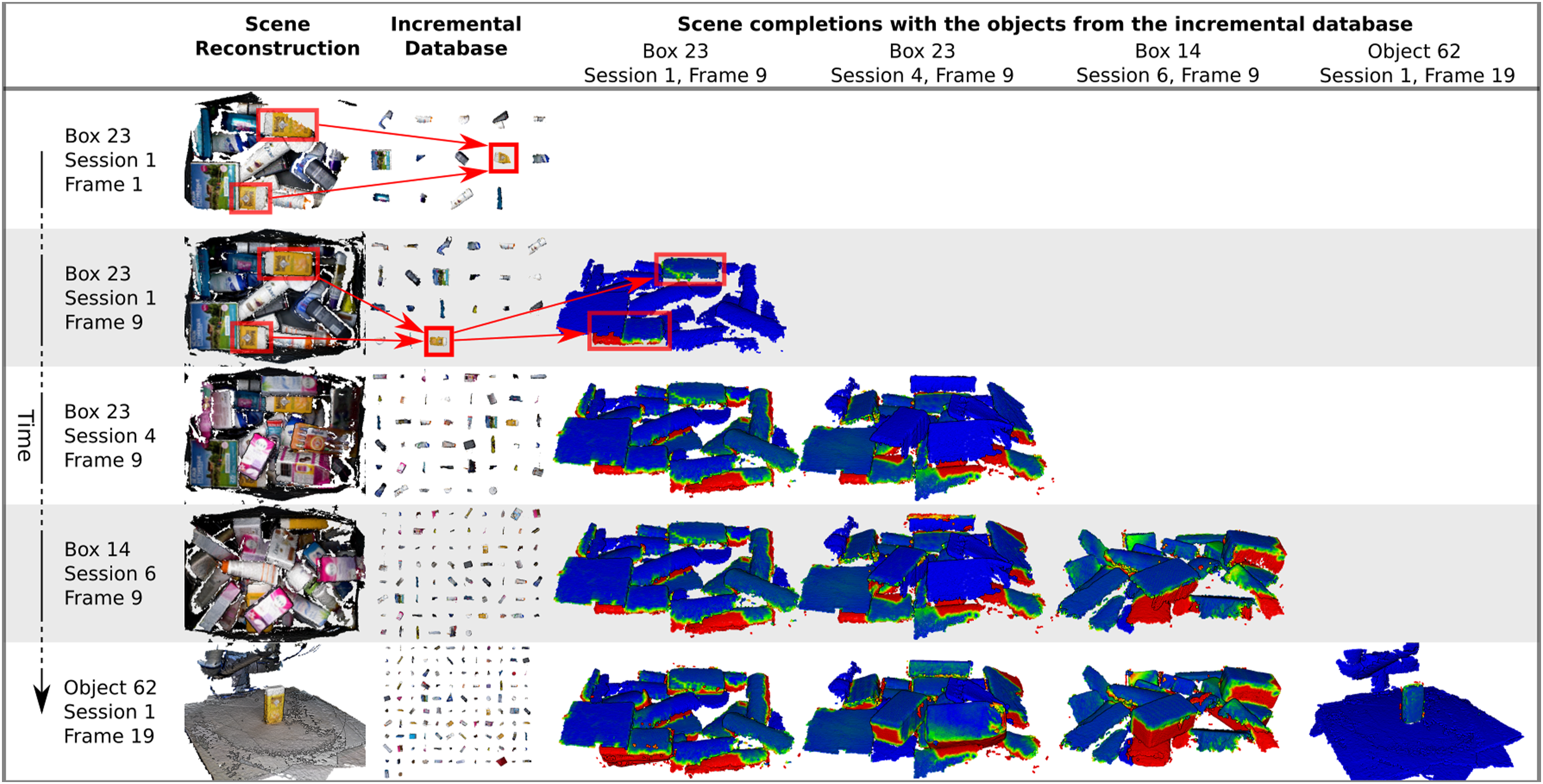

4.1.3. Garage

The garage dataset contains five sequences, split into nine sessions, recorded with a custom-built RGB-D-I sensor. We combined a FLIR BlackFly S 1.6 MP RGB camera, a pico monstar time-of-flight depth camera, and an ADIS-16448 IMU. These sensors are synced in time and triggered by a microcontroller with the method described by Tschopp et al. (2020) and calibrated using the kalibr software (Rehder et al., 2016).

The RGB and the IMU data were processed using maplab (Schneider et al., 2018) to generate optimized camera poses, for every sequence. As our approach currently still relies on localized cameras and we are not using our segment matches to improve the localization, we cannot just use a visual-inertial state estimation framework, as this suffers from too much drift that would corrupt our segmentation maps. Hence, maplab gives us globally optimized camera poses per sequence. As four sequences still contain substantial amount of drift and we end up with double surfaces in the scene reconstructions, we split these into two sessions each. Three sequences are recorded indoors (Sessions 1–6), one sequences outdoors (Sessions 7–8), and one sequence starts outdoors and transitions to the indoor part of the garage (Session 9). The scene reconstructions of the nine sessions are shown in a top-down view in Figure 11.

Figure 11.

Top-down view on the reconstructed scenes of the garage dataset Sessions 1–9. For visualization purposes, we put all the sessions into the same frame. Each session is colored differently and we highlight some regions and show the reconstructions from individual sessions. The right side is the outside part of the garage.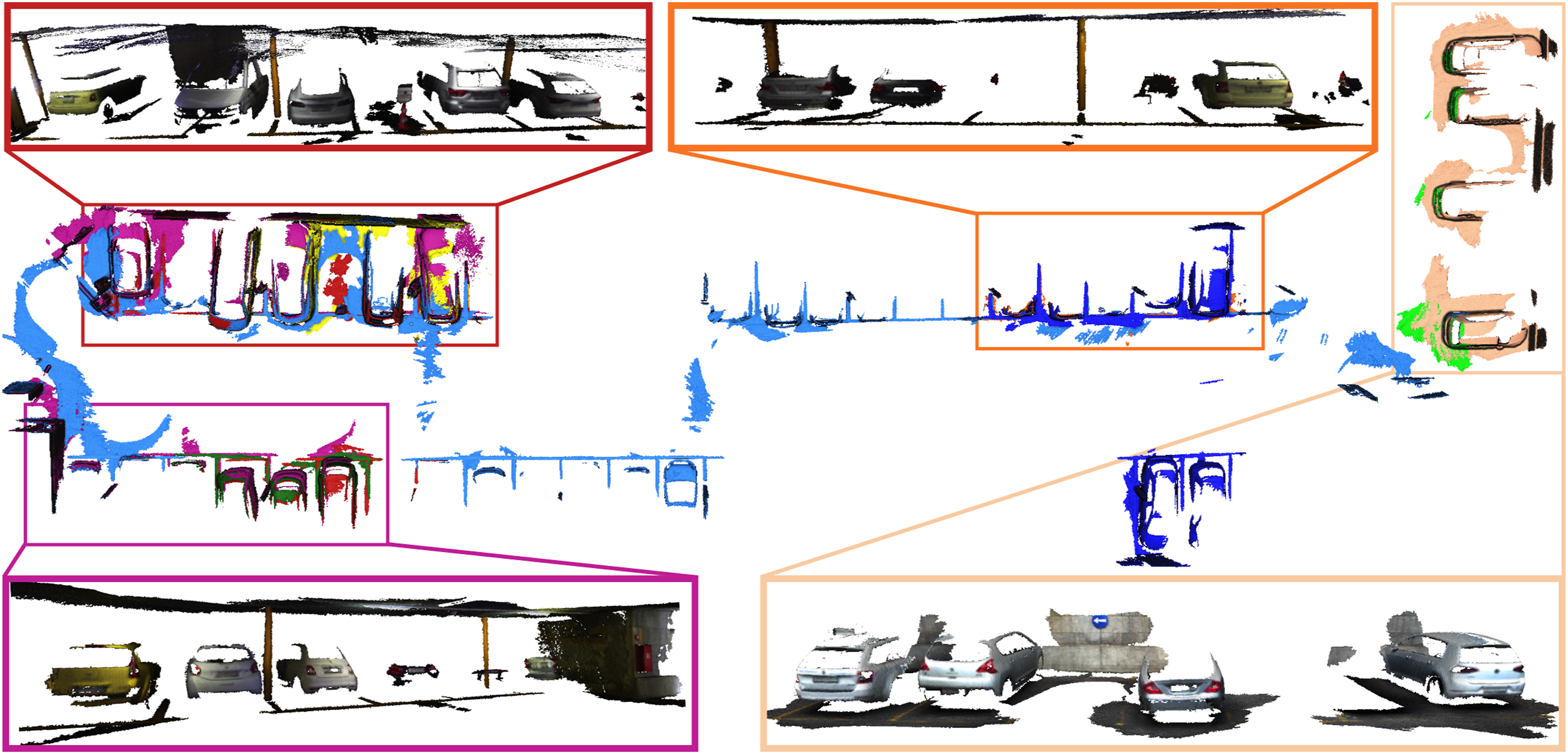

The floor in the garage is very dark, except for the line markings, therefore, we only get depth camera returns when we point the camera downwards, this is similar as in the Tango dataset.

4.2. Metrics

In order to evaluate our system, we have compared the number of detected instances, segment matches, and merged segments with the ground truth data. Furthermore, we analysed the performance by timing each step of the pipeline.

4.2.1. Ground truth annotation

To be able to evaluate the system properly, we first created a tool to manually annotate each segment in the segmentation map. In this process, we assign the same label to the same objects that appear in the same, or multiple, sessions. This way we can automatically obtain the number of ground truth matches and merges by computing all the positive and negative segment pairs, that is, ones that belong to the same ground truth label and ones that do not. Segments that contain too few points or belong to the background are assigned a special label and are not considered in the evaluation (in our case floors, walls, and ceiling). Furthermore, if the same object is observed from two different sides, without any overlap, these two segments would get the same label, however, our system would not be able to merge them. Additionally, even if we have small indistinct parts of the object, we still label them with the proper label meaning that the ground truth can also contain merges which are impossible. This should be taken into account when interpreting the results of our evaluation.

4.2.2. Matching and merging

By having the ground truth annotations, we can extract all the segment pairs that belong together. Therefore, we can use these pairs to evaluate the correctness of our matching and merging. Based on the matching results that we obtain from our incremental database, we can count the number of correct matches, that is, true positives (TP) and true negatives (TN), as well as incorrect matches, that is, false positives (FP) and false negatives (FN). Furthermore, we can count the number of correct (CO), partial (PA), missing (MI), and wrong (WR) merges. A match is considered successful if the ICP algorithm converged and the final error is below a certain threshold. Furthermore, if a single object is split into multiple partial merges, we count this as one partial merge.

4. 2.3. Runtimes

We time every major step of our pipeline individually for each new segment that we process. Therefore, we show the timings per segment, as well as the average times for each algorithm step.

4. 3. Evaluation

We show the results obtained by running our incremental database on different datasets and compare it with the results obtained in our previous work (Furrer et al., 2018). A summary of the number of available segments, how many of them are identified as mergeable, and matching and merging results are presented in Table 1.

Table 1.

Ground truth merge count versus modelify merge count for the different datasets.

Dataset	Segments			Matches (%)				Merges
Dataset	Total	Mergeable	Merged	TP	TN	FP	FN	CO	PA	MI	WR	GT
Tango 1	102	13	8	9	66	24	1	3	0	1	0	4
Tango 2	143	20	3	7	61	25	7	0	1	4	0	5
Tango 3	77	15	6	9	75	9	7	1	1	2	0	4
Tango 1–3	322	48	34	10	66	18	6	2	4	1	0	7
Tango 1–3 M	322	48	38	—	—	—	—	3	3	1	0	7
Tango 1–3 O	322	48	27	—	—	—	—	1	5	1	1	7
Tango 1–3 P	322	92	37	5	69	17	9	0	7	2	0	9
Tango 1–3 P M	322	92	37	—	—	—	—	0	7	2	0	9
Box 13	53	53	29	2	94	0	4	4	6	4	0	14
Box 14	72	72	46	2	94	0	4	3	8	4	0	15
Box 23	91	91	68	2	96	0	2	7	10	4	0	21
Box 13, 14, 23	216	216	156	1	97	0	2	6	23	6	0	35
Box 13, 14, 23 M	216	216	163	—	—	—	—	6	23	6	0	35
Box 13, 14, 23 OB	236	236	167	1	97	0	2	7	24	6	0	37
Box 13, 14, 23 OB M	236	236	174	—	—	—	—	9	23	5	0	37
Garage 1–9	331	98	50	3	55	41	1	5 (6)*	8	6	1 (0)*	21
Garage 1–9 M	331	98	50	—	—	—	—	5 (6)*	8	6	1 (0)*	21

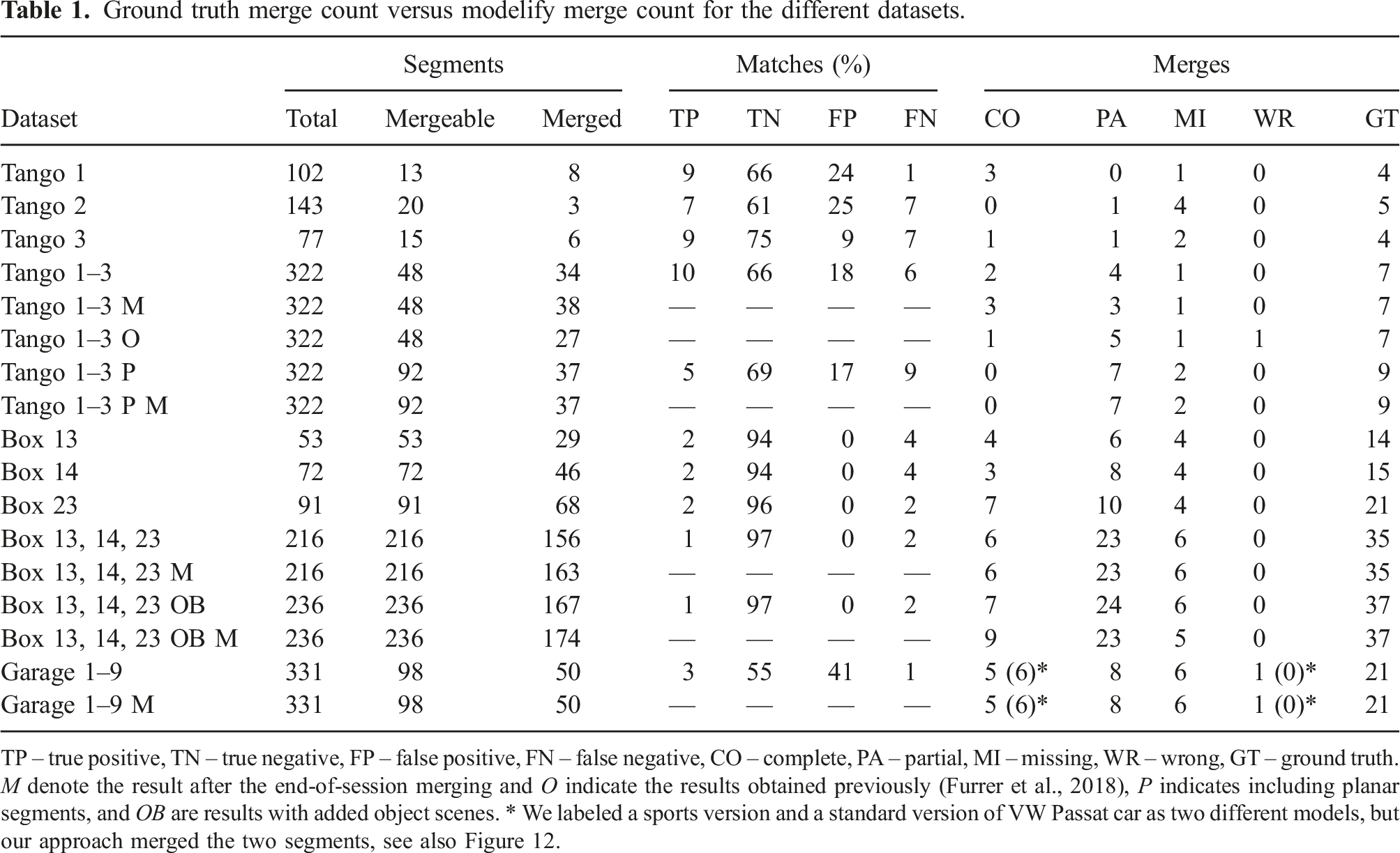
TP – true positive, TN – true negative, FP – false positive, FN – false negative, CO – complete, PA – partial, MI – missing, WR – wrong, GT – ground truth. M denote the result after the end-of-session merging and O indicate the results obtained previously (Furrer et al., 2018), P indicates including planar segments, and OB are results with added object scenes. * We labeled a sports version and a standard version of VW Passat car as two different models, but our approach merged the two segments, see also Figure 12.

We list numbers for matches and merges in the individual Tango and CLUBS sessions, as they contain repeating instances in one session and for the Garage dataset we only report numbers at the end, as there are no repeating objects within one session. While the segmentation map typically oversegments the scene, our matching and merging results are very satisfying. In the Tango datasets, we kept the old segmentation approach in all the experiments, which extracts some undersegmented parts, such as the helmets (see Figure 3), to have comparable results, even though with the new convexity measure we can successfully segment these objects. Matching numbers for the end-of-session merging step (datasets marked with M) are excluded since it is not possible to count them properly, as the end-of-session merging is allowed to match and merge already merged segments.

We get the best possible result on the Tango 1 session, as we get three out of four repeating objects completely merged. The missing merge is not possible to merge with our approach, there is no overlap of the segments, as they originate from the same instance, visible in Session 1 in Figures 8 and 9, where the square (red) chair is split into two segments. Slightly worse results we get in the Tango 3 session, where we only merge the three white chairs completely, and we partially match the fire extinguishers and the gas tanks. The two missing merges are again impossible matches for our system, as the cow and the square chair consist of multiple segments. In the Tango 2 dataset, we miss some merges, the worse performance here can be explained with the noisier poses in this session, leading to non-smooth surfaces, with sometimes even multiple surfaces in the reconstruction.

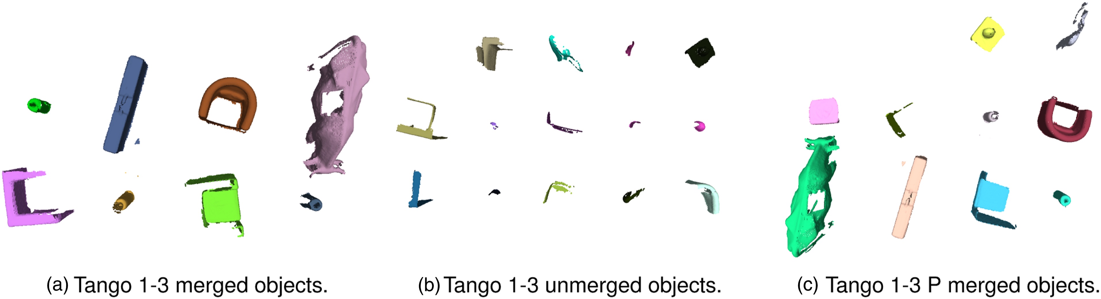
When using our method without the end-of-session merging Tango 1–3, we can merge the gas tanks and the gray box models with all the mergeable segments. The fire extinguishers and the cube chair are split into two models as can be seen in Figure 13(a) where we show all merged objects. The cow, fire extinguishers, the round chair, and the cube chair are missing 3, 2, 4, and 3 mergeable segments, visible in Figure 13(b). In the mergeable but unmerged segments, we additionally have two segments that are not repeating (within the mergeable segments): a helmet together with a cushion of the round chair (top row right), and a helmet (middle row right). Our method fails at merging the little white cylindrical container segments that are mergeable in Session 1 and 2. In the bottom of Figure 9, we also show how the merged segments can be used to complete the reconstructed scenes.

Figure 12.

A sports version and a default version of a VW Passat (labeled as different models in the ground truth), are merged into one model. The highlighted parts show that the merging process improves noisy regions.

Figure 13.

Merged objects in the tango dataset, Tango 1–3 and Tango 1–3 P. In our previous paper: cow (3), round chair (10), fire-extinguisher (4 in 2 objects), gas cylinder (4), box (2), cube chair (2), and 1 wrong merge. Now in (a): fire-extinguisher (8 in 2 objects), box (2), round chair (11), cow (4), cube chair (4 in 2 objects), gas cylinder (5), and no wrong merges. If we use the end-of-session merging, the round chair model is fused with three additional segments and the cube chair with 1 additional segment. In (b), we show the mergeable segments that are not merged with any other segment from the Tango dataset without flat objects (Tango 1–3). In (c), we depict the merged objects with including flatter segments Tango 1–3 P: cow (7 in 2 objects), round chair (12), fire-extinguisher (4), gas cylinder (4), box (2), cube chair (4 in 2 objects), seat cushion (4 in 2 parts).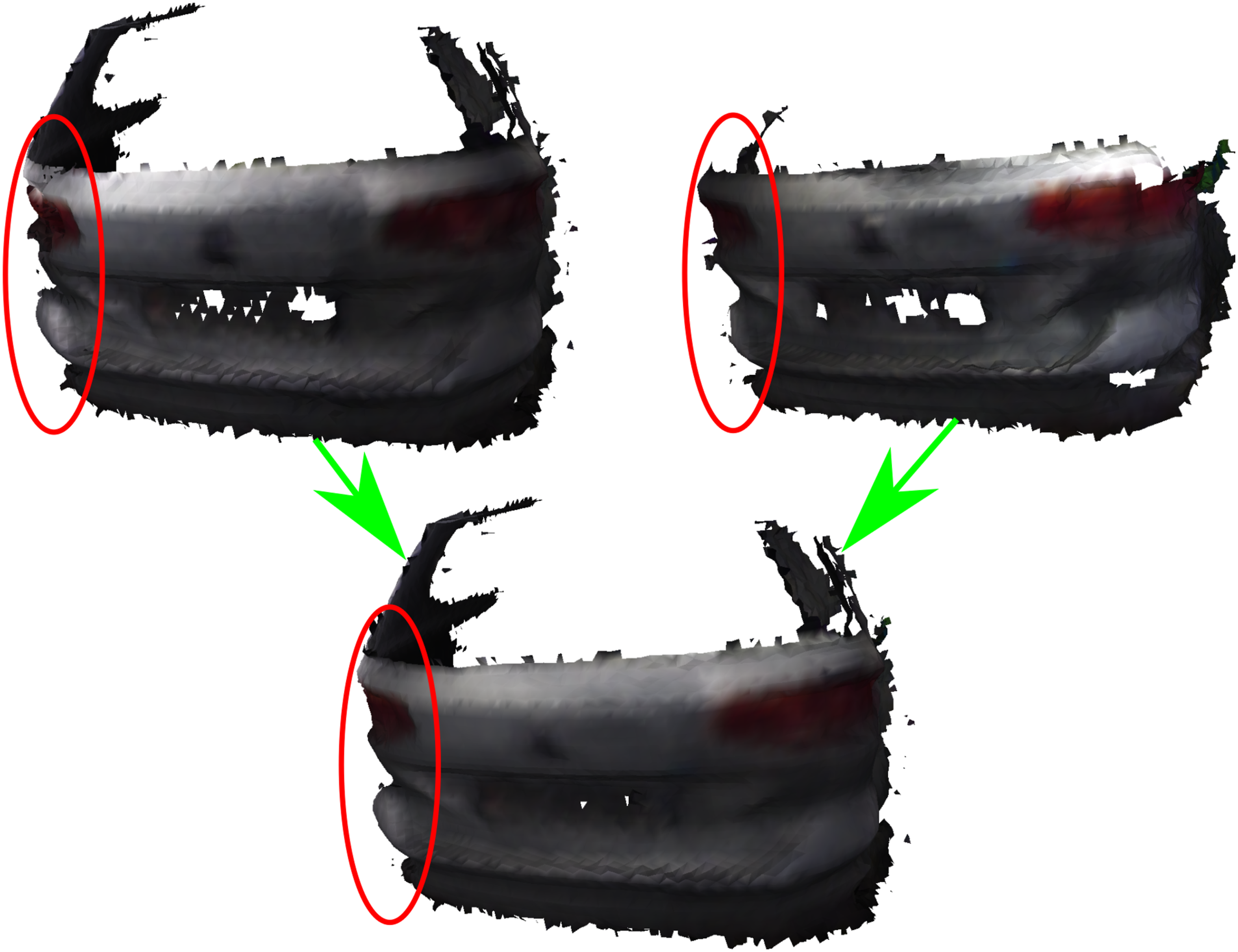

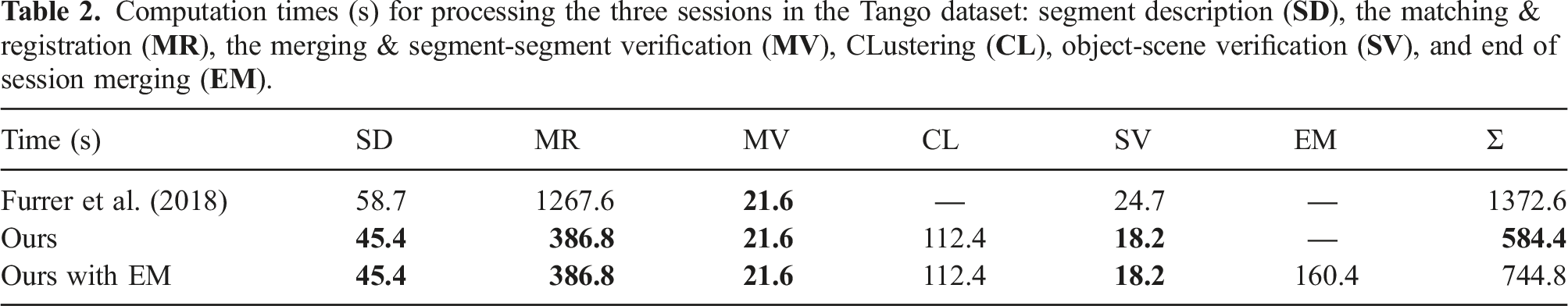
When applying the end-of-session merging Tango 1–3 M, we can additionally merge the remaining three round chair segments. And when we compare Tango 1–3 M with Tango 1–3 O, we can see that with our new method we can get more completely merged object models, have no wrong merges while being substantially faster, as shown in Table 2. If we additionally allow segments that are more planar, we can almost double the mergeable segments, as noted in Tango 1–3 P. To avoid getting wrong merges, we had to tighten our object-scene verification parameters, as almost planar segments can geometrically match to many surfaces. We show that we additionally get merged cushions of the round chair in Figure 13(c), one with and one without a helmet. But we also lose some of the previous successfully merged segments due to the tighter object-scene verification parameters. 2D features contribute to around half of the correct matches in this dataset, which is also one of the reasons for obtaining slightly better results compared to Tango 1–3 O.

Table 2.

Computation times (s) for processing the three sessions in the Tango dataset: segment description (SD), the matching & registration (MR), the merging & segment-segment verification (MV), CLustering (CL), object-scene verification (SV), and end of session merging (EM).

Time (s)	SD	MR	MV	CL	SV	EM	$Σ$
Furrer et al. (2018)	58.7	1267.6	21.6	—	24.7	—	1372.6
Ours	45.4	386.8	21.6	112.4	18.2	—	584.4
Ours with EM	45.4	386.8	21.6	112.4	18.2	160.4	744.8

In the CLUBS dataset, we selected three box scenes at different stages in the box emptying process. In the first box, box 13, we selected iterations 25, 18, 15, and 0, to evaluate our system. In the second, box 14, we selected iterations 19, 8, 1, 0 and in the third, box 23, 37, 33, 28, 14, 9, and 4. The selection of iterations was done based on objects that are visible at that point in that specific box. Since in consecutive iterations there is only one object difference in the box, selecting each iteration would not be so interesting for our experiment. Therefore, we picked the iterations where the change between them is significant enough, for the same box, to add at least a few of the new objects but not so drastic that all the previous objects are occluded.

In contrast to the other two datasets, box scenes are recorded in a specific setup where the camera is looking from above. When our segmentation is applied to such a dataset, most of the segments that are extracted are flat faces of different products contained in the box. Therefore, in this case, we allowed the database to accept completely planar segments. Furthermore, we only used 2D features for matching since planar segments do not provide any geometrically distinctive 3D features. The scene evaluation is not a good measure for planar segments, therefore, we can only accept the best matches. For this reason, we aimed at getting very low false positive matches. This also results in having slightly higher false negative matches compared to the other datasets. While we are able to merge segments originating from a single depth frame, as indicated in Figure 10, we are missing some matches in favor of avoiding wrong merges. Nevertheless, the numbers show that a large portion of the discovered object segments are matched at least once to a segment from the same household object (156 out of 216). With the end-of-session merging strategy, we achieved even slightly better results (163 out of 216). If we start by processing 40 singulated object scenes (20 objects in two orientations) first, and then insert them into a database before processing the box scenes, we can improve these numbers even more. We show the resulting 3D models of processing solely the object scenes in Figure 14. The object models after end-of-session merging of the box scenes only and with processing the object scenes first are depicted in Figure 15.

Figure 14.

A set of the CLUBS objects generated by merging the models of the two object scenes. In the CLUBS dataset, each object was scanned twice. After a first scan, each object was rotated upside down to also capture the bottom side of the object.

Figure 15.

The 48 merged objects from the CLUBS dataset after processing the box scenes with end-of-session merging in (a) and the 47 merged objects after processing the 40 object scenes of the 20 objects in Figure 14, followed by processing the three box scenes and the end-of-session merging in (b). While the quality of the object models degraded compared to the ones extracted solely in object scenes, these models still provide good approximations of the real objects. The models can be re-detected in new scenes, and are accurate enough to perform manipulation tasks.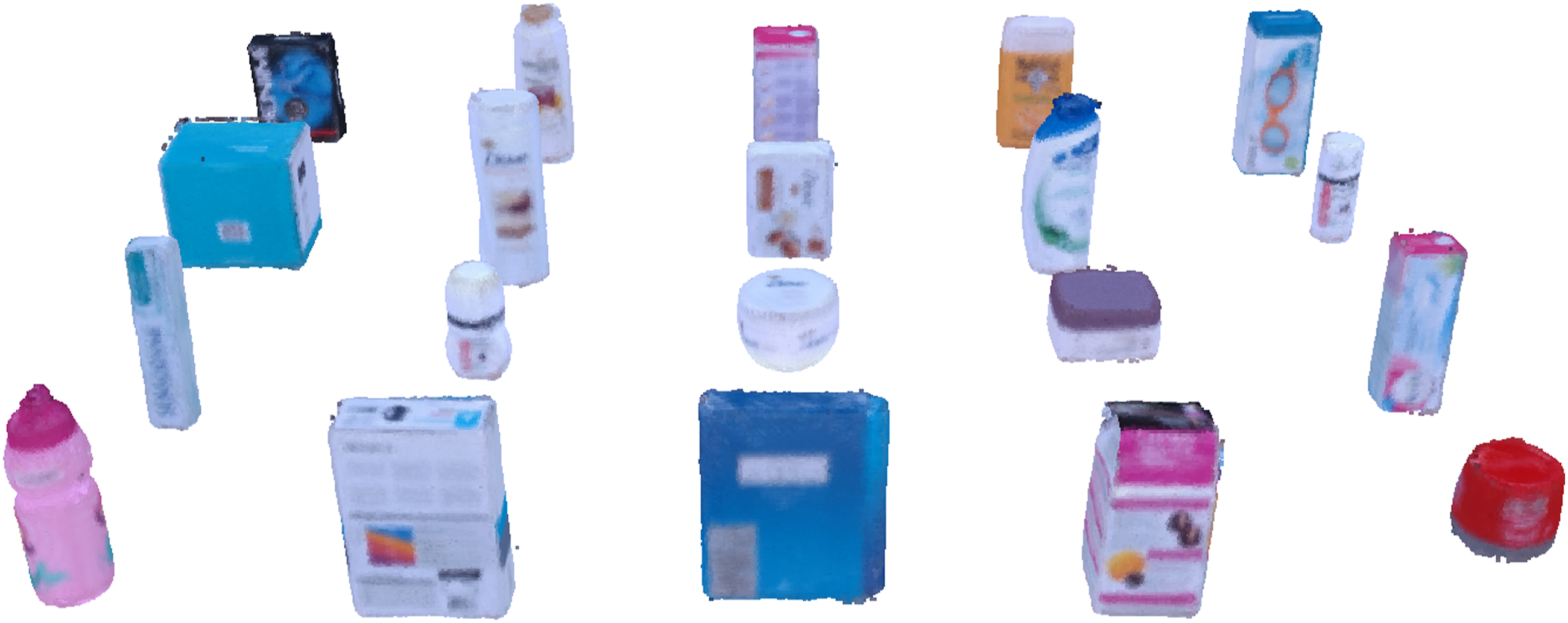

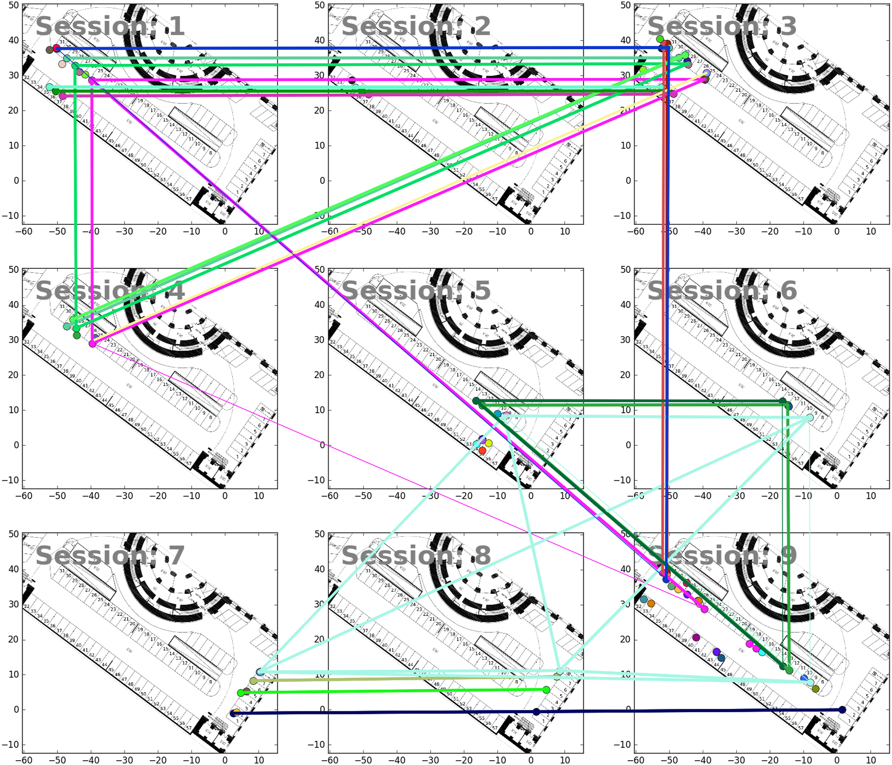
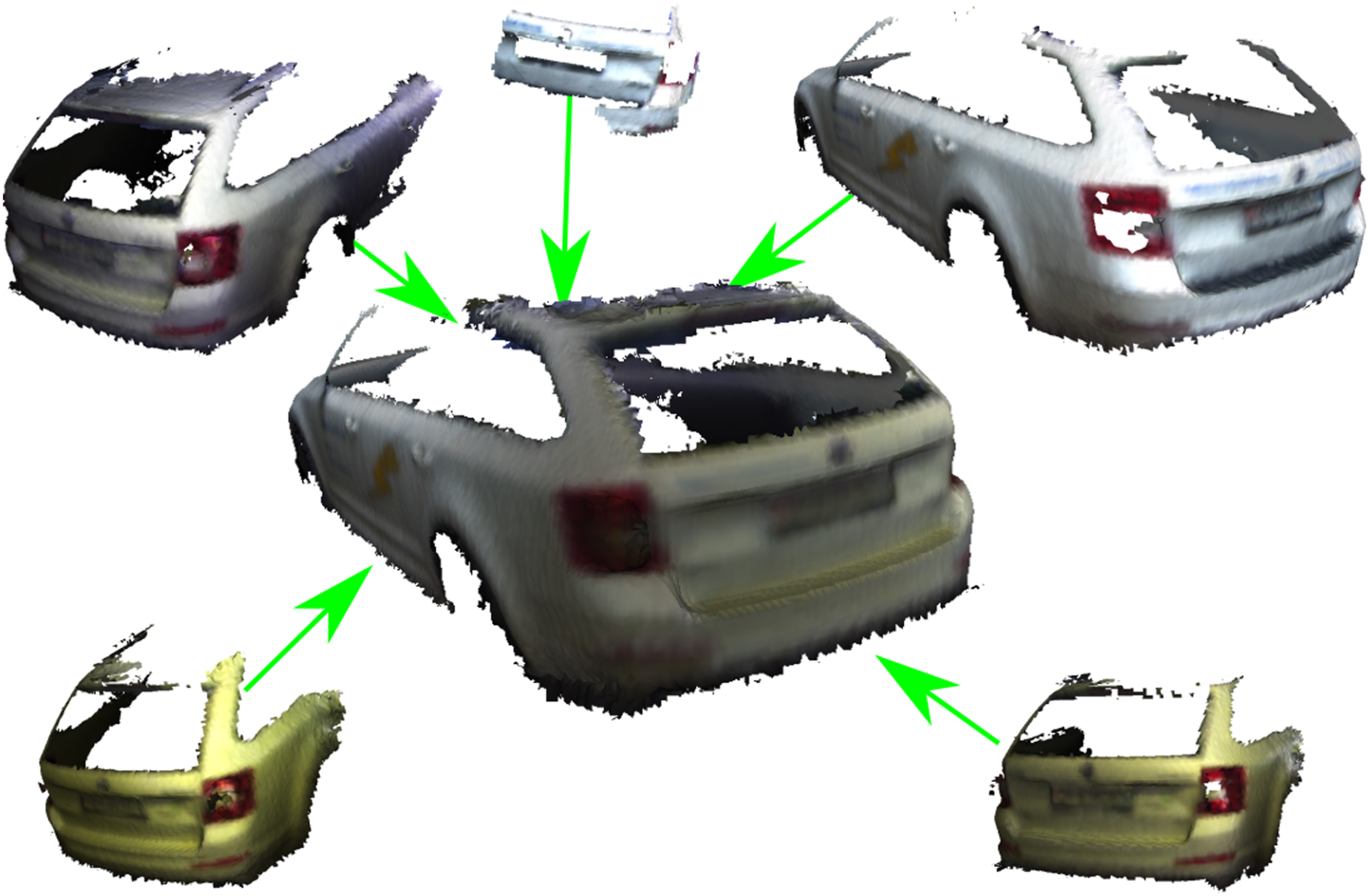
For the Garage dataset, we only show results after processing all the sessions in the dataset, as there is no session with repeating car models (except for Session 9, but we did not label it as a repeating model, as the model is slightly different, Table 1 *). Similar as in the Tango dataset, our segmentation map tends to oversegment the scene, as is visible in Figure 16. Figure 17 shows which segments from the different sessions got matched by our approach. We added the floorplan of the garage in the background and aligned all the sessions to the floorplan frame for visualization purposes (the processing was done in the original session frames). While we are missing six potential merges, we are able to get the maximum possible number of segments merged into one model for five objects, eight models are partially merged and 1 merge is wrong. The wrong merge is depicted in Figure 12 and is only wrong as we labeled two different models of one car type differently (Table 1 *), if the two segments would have been assigned to one model this wrong merge would be counted as a completed merge, as shown in Table 1. Both, 2D and 3D features are not very distinctive in this dataset, as cars have very similar sizes and keypoints appear at similar places on different car models (e.g., on lights, door handles, license plates). Therefore, we accept more matches and allow to have a large number of false positives. However, we can be strict in the scene evaluation. Most of the matches were provided by the 2D features, as they tend to match more often and often give better initial alignments. Our method managed to merge segments originating from two different Skoda Octavia cars, as shown in Figure 18. The cars have different colors and were observed under very different lighting conditions, visible also in the figure. As shown in Figure 12, the TSDF-based merging of the two geometric segments reduces noise at overlapping areas in the merged object.

Figure 16.

The reconstruction of the garage Session 3, with the segmentation map and the ground truth segments (purple indicates background). (a) Scene reconstruction, (b) Segmentation map, (c) Ground truth.

Figure 17.

Clusters formed while evaluating all nine sessions of the garage dataset. The segments (circles) are overlaid on a floor plan of the garage. All the sessions are transformed into a common frame to better visualize the correctness of the proposed clusters. Note that the pink cluster between Sessions 5–9 is a cluster of two identical car models as shown in Figure 18.

Figure 18.

The method could successfully merge segments of two different Skoda Octavia models, despite the different lighting conditions. The two segments on top right were recorded in the outside part of the garage (Sessions 7 and 8) and are from a different car than the other three segments recorded in the inside part of the garage (Session 5, 6, 9).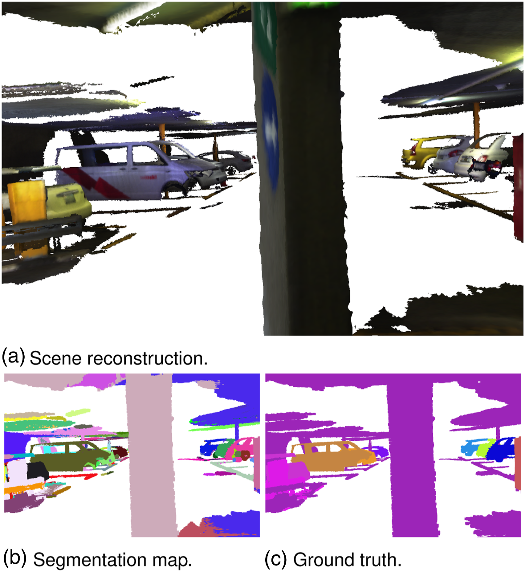

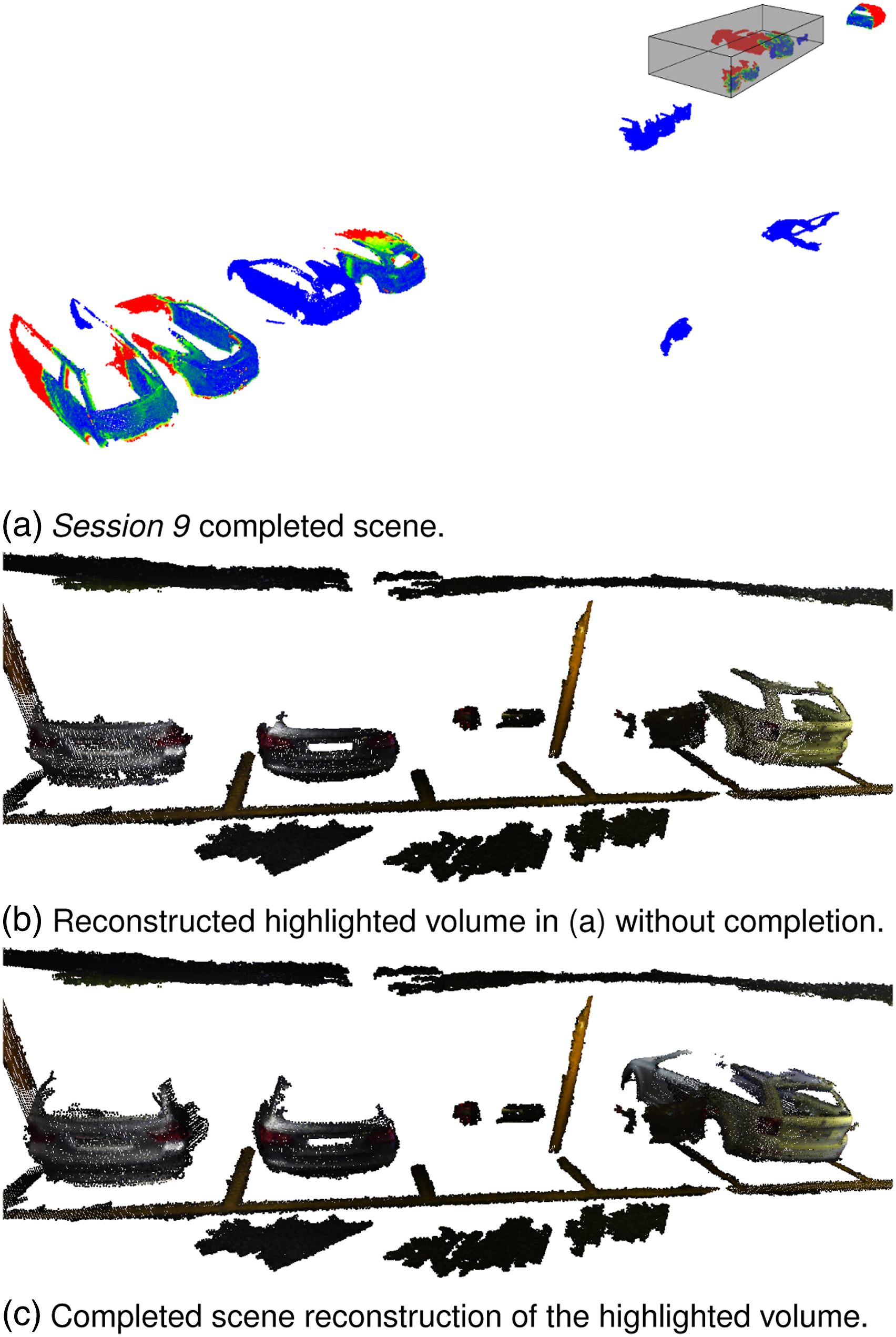
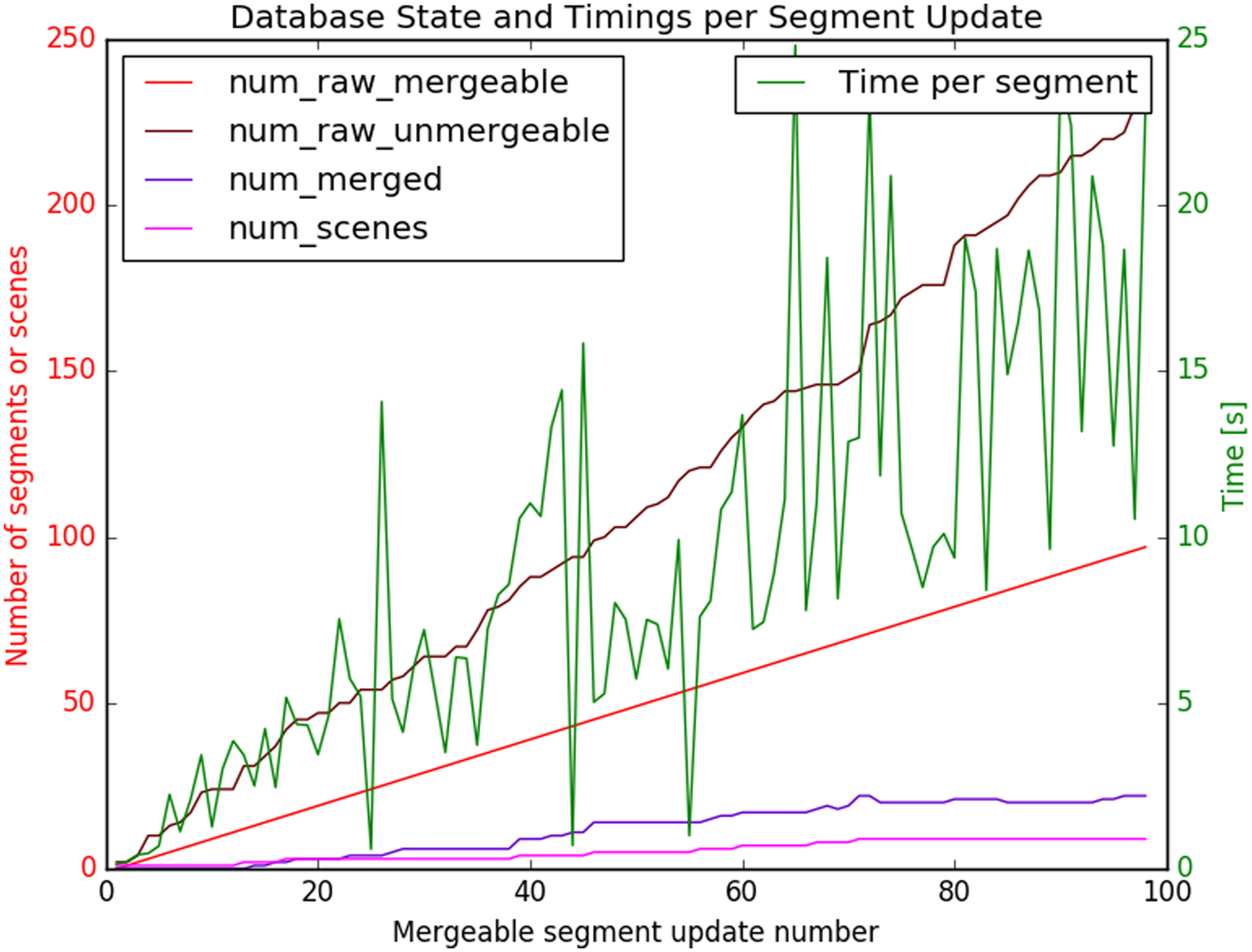
In Figure 19, we show the models of the merged cars. Using these models, we demonstrate in Figure 20 that we can substantially complete scenes. The results are presented for Session 9 with the information gained over the other eight sessions. In Figure 21, we show that the overall processing time per segment scales linearly with the amount of segments in the database.

Figure 19.

The merged car models from all the sessions of the garage dataset.

Figure 20.

The original (non-background) segments of Session 9 of the garage dataset (in blue) could be corrected and completed by using the merged segments from the other sessions (green to red) (a). The impact of the scene completion of the highlighted region in (a) is shown in (b) and (c).

Figure 21.

Timings per mergeable segment update received from the segmentation maps of the nine sessions in the garage dataset. The processing times per segment increase linearly with the amount of num_raw_mergeable segments. Segments are published at the end of each session, indicated with the increase in num_scenes.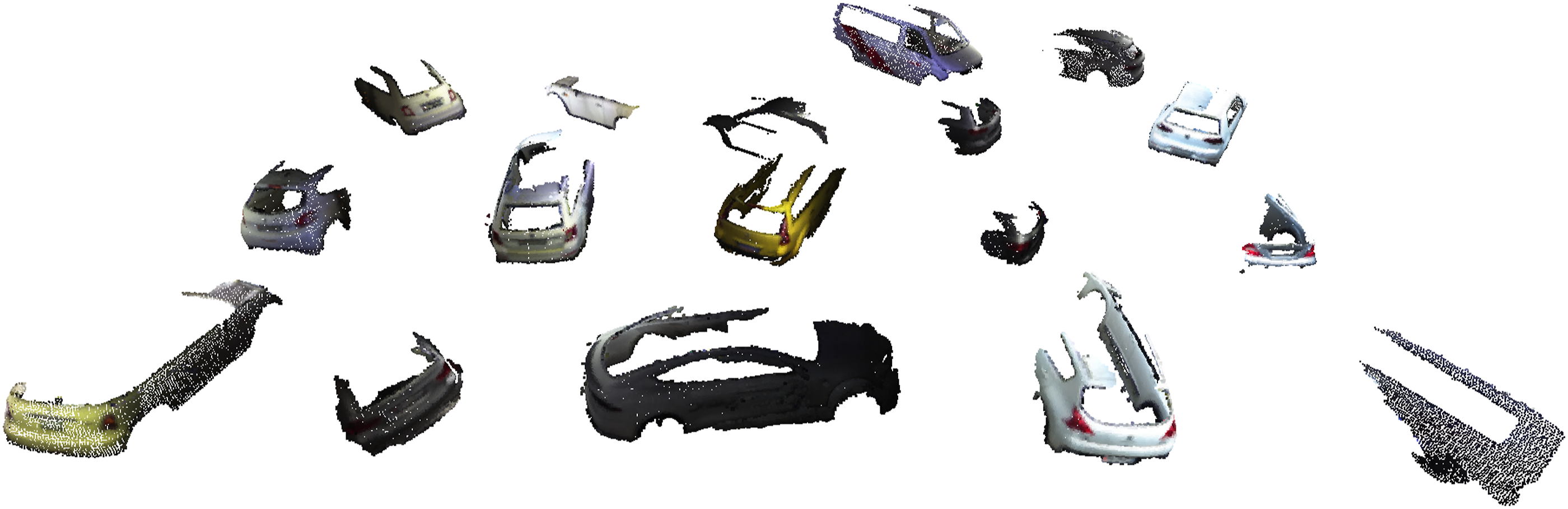

4.4. Discussion

We have shown that our system can perform well on different types of data, however, there are some inherit limitations to what we can achieve. Some of these are discussed below.

4.4.1. Segmentation

Even though our geometric segmentation performs well for certain environments and objects, it still does not capture the notion of an object. Furthermore, we are able to segment convex regions but if these are consistently under segmenting the objects there is currently no way to separate them in the segmentation map. To ensure that our approach is applicable in completely unknown environments, we focused on a purely geometric approach. However, different segmentation techniques could be used to provide better segments, and if the method is applied in an environment where semantic information can be learned, semantic instance segmentation mapping methods (Grinvald et al., 2019) could be employed. Adding semantics could additionally be used to exclude segments with certain classes like person or cat, which might be undesired in some maps or tasks.

4.4.2. Memory consumption

We based our implementation on Voxblox (Oleynikova et al., 2017) and therefore suffer from the same memory limitations. Since we are keeping the whole map as a TSDF grid in the memory, running a very large dataset (that does not revisit the old locations) might hit memory limits. To address this issue, sub-mapping and keyframing methods could be used to reduce the memory requirements, as shown by Millane et al. (2018). Another approach would be to work only on a local map, for example, using a sliding window (i.e., a volume around the current position).

4.4.3. Runtime scalability

As shown in Section 4.3, matching step scales linearly with the number of segments in the database. Since we match the new segment to all the segments in the database, our approach takes a considerable amount of time, once the database gets large. We can parallelize segment-segment matching and evaluations, but this still does not scale with very large databases. An approach, like Bag-of-words (Sivic and Zisserman 2009) could be used to reduce the matching time.

4.4.4. Accurate poses required

In our approach, we assume that we have very accurate camera pose estimates. If this is not the case, the segments we obtain are very noisy and hard to match and register. Furthermore, the TSDF evaluations will have a larger RMSE and will fail more often. That is why for our datasets poses are optimized in a post-processing step.

5. Conclusion

We presented a system that is able to extract and fuse object segments on a variety of RGB-D datasets. The use of 2D features projected to their 3D location generally outperforms the use of 3D information alone, while 3D features are still valuable for segments with little texture. A combination also proved to be very useful to handle strong illumination changes. The error histogram-based verification step helped to reject segment merges that had low RMSE. The clustering approach makes our method scale linearly with the amount of segments for the matching and merging part, with only few missing merges. Using our approach, we showed that we can substantially complete scenes with merged object models. The results show that our verification steps can minimize the number of wrong merges. This opens possibilities to solve robotic spatial understanding for physical interaction (e.g., manipulation tasks) in initially completely unknown scenes. With our system, a robot is able to build its own object database over time.

Our system is very well suited to be combined with a Simultaneous Localization and Mapping (SLAM) system as the object-based representation. To overcome limitations of our segmentation maps, introducing a co-observability measure would allow to merge segments that have been observed at identical relative poses multiple times. Similarly, it would be beneficial to introduce a measure to split a segment such that if one segment matches to multiple non-overlapping segments with inconsistent relative transformations, it is likely that it belongs to different physical entities. As we focused on completely unknown scenes, we restricted the presented approach to use a purely geometrical segmentation. Nevertheless, we strongly believe that combining geometrical knowledge with data-driven approaches will improve image and scene segmentation.

Footnotes

Declaration of conflicting interests

The author(s) declared no potential conflicts of interest with respect to the research, authorship, and/or publication of this article.

Funding

The author(s) disclosed receipt of the following financial support for the research, authorship, and/or publication of this article: This work was supported by the Amazon Research Awards program, the Swiss National Science Foundation (SNF), within the National Centre of Competence in Research on Digital Fabrication, and the Swiss Commission for Technology and Innovation (CTI).

ORCID iDs

Fadri Furrer

Tonci Novkovic

Notes

References

Aldoma

Marton

Tombari

, et al. (2012) Tutorial: point cloud library: three-dimensional object recognition and 6 dof pose estimation. IEEE Robotics & Automation Magazine 19(3): 80–91.

Ambruş

Bore

Folkesson

, et al. (2014) Meta-rooms: building and maintaining long term spatial models in a dynamic world. In: 2014 IEEE/RSJ International Conference on Intelligent Robots and Systems, Chicago, IL, September 2014. pp. 1854–1861.

Ambrus

Bore

Folkesson

, et al. (2017) Autonomous meshing, texturing and recognition of object models with a mobile robot. In: 2017 IEEE/RSJ International Conference on Intelligent Robots and Systems (IROS), Vancouver, BC, September 2017. pp. 5071–5078.

Arun

Huang

Blostein

(1987) Least-squares fitting of two 3-d point sets. IEEE Transactions on Pattern Analysis and Machine Intelligence 9(5): 698–700.

Avetisyan

Dahnert

Dai

, et al. (2019) Scan2cad: learning cad model alignment in rgb-d scans. In: Proceedings of the IEEE Conference on Computer Vision and Pattern Recognition, Long Beach, CA, USA, 15-20 June 2019, pp. 2614–2623.

Besl

McKay

(1992) A method for registration of 3-d shapes. IEEE Transactions on Pattern Analysis and Machine Intelligence 14(2): 239–256.

Billard

Kragic

(2019) Trends and challenges in robot manipulation. Science 364(6446): eaat8414.

Bolya

Zhou

Xiao

, et al. (2019) YOLACT: real-time instance segmentation. CoRR abs/1904.02689.

Chen

Wang

Pang

, et al. (2019) MMDetection: open MMLab detection toolbox and benchmark. CoRR abs/1906.07155.

10.

Chen

(2017) Object-level motion detection from moving cameras. IEEE Transactions on Circuits and Systems for Video Technology 27(11): 2333–2343.

11.

Chen

Medioni

(1991) Object modeling by registration of multiple range images. In: Proceedings of 1991 IEEE International Conference on Robotics and Automation, Sacramento, CA, April 1991. pp. 2724–2729 vol.3.

12.

Correll

Bekris

Berenson

, et al. (2018) Analysis and observations from the first amazon picking challenge. IEEE Transactions on Automation Science and Engineering 15: 172–188.

13.

DeTone

Malisiewicz

Rabinovich

(2018) Superpoint: self-supervised interest point detection and description. In: Proceedings of the IEEE Conference on Computer Vision and Pattern Recognition Workshops, Salt Lake City, UT, June 2018. pp. 224–236.

14.

Dongen

(2000) A Cluster Algorithm for Graphs. Information Systems [INS] 10(R 0010).

15.

Dubé

Cramariuc

Dugas

, et al. (2019) Segmap: segment-based mapping and localization using data-driven descriptors. The International Journal of Robotics Research 39: 339–355.

16.

Ekvall

Kragic

Jensfelt

(2007) Object detection and mapping for service robot tasks. Robotica 25(2): 175–187.

17.

Fehr

Furrer

Dryanovski

, et al. (2017) TSDF-based change detection for consistent long-term dense reconstruction and dynamic object discovery. In: 2017 IEEE International Conference on Robotics and Automation (ICRA), Singapore, May 2017. pp. 5237–5244.

18.

Fischler

Bolles

(1981) Random sample consensus: a paradigm for model fitting with applications to image analysis and automated cartography. Communications of the ACM 24(6): 381–395.

19.

Frey

Dueck

(2007) Clustering by passing messages between data points. Science 315(5814): 972–976.

20.

Furrer

Novkovic

Fehr

, et al. (2018) Incremental object database: building 3d models from multiple partial observations. In: IEEE/RSJ International Conference on Intelligent Robots and Systems, Madrid, Spain, October 2018. pp. 6835–6842.

21.

Grinvald

Furrer

Novkovic

, et al. (2019) Volumetric instance-aware semantic mapping and 3d object discovery. IEEE Robotics and Automation Letters 4(3): 3037–3044.

22.

Guo

Bennamoun

Sohel

, et al. (2014) 3d object recognition in cluttered scenes with local surface features: a survey. IEEE Transactions on Pattern Analysis and Machine Intelligence 36(11): 2270–2287.

23.

Gupta

Girshick

Arbeláez

, et al. (2014) Learning rich features from rgb-d images for object detection and segmentation. In: European Conference on Computer Vision. Cham: Springer, 345–360.

24.

Gkioxari

Dollár

, et al. (2017) Mask r-cnn. In: IEEE International Conference on Computer Vision, Venice, Italy, October 2017, pp. 2980–2988.

25.

Zhang

Ren

, et al. (2016) Deep residual learning for image recognition. In: Proceedings of the IEEE conference on computer vision and pattern recognition, Honolulu, HI, July 2016, pp. 770–778.

26.

Herbst

Henry

Fox

(2014) Toward online 3-d object segmentation and mapping. In: 2014 IEEE International Conference on Robotics and Automation (ICRA), Hong Kong, China, 31 May–07 June 2014, pp. 3193–3200.

27.

Hou

Dai

Nießner

(2019) 3d-sis: 3d semantic instance segmentation of rgb-d scans. In: The IEEE Conference on Computer Vision and Pattern Recognition (CVPR), Long Beach, CA, USA, 15-20 June 2019, pp. 4421–4430.

28.

Huang

Gong

, et al. (2019) Mask scoring r-cnn. In: The IEEE Conference on Computer Vision and Pattern Recognition (CVPR), Long Beach, CA, USA, 15-20 June 2019, pp. 6409–6418.

29.

Kirillov

Girshick

, et al. (2019) Panoptic segmentation. In: Proceedings of the IEEE Conference on Computer Vision and Pattern Recognition, Long Beach, CA, USA, 15-20 June 2019, pp. 9404–9413.

30.

Krotkov

Hackett

Jackel

, et al. (2017) The darpa robotics challenge finals: results and perspectives. Journal of Field Robotics 34(2): 229–240.

31.

Lin

Goyal

Girshick

, et al. (2017) Focal loss for dense object detection. In: Proceedings of the IEEE international conference on computer vision. Venice, Italy, October 2017. pp. 2980–2988.

32.

Liu

Dai

(2017) Efficient global 2d-3d matching for camera localization in a large-scale 3d map. In: 2017 IEEE International Conference on Computer Vision (ICCV). Venice, Italy, October 2017. pp. 2391–2400.

33.

Lorensen

Cline

(1987) Marching cubes: a high resolution 3d surface construction algorithm. ACM SIGGRAPH Computer Graphics 21: 163–169.

34.

Lowe

(2004) Distinctive image features from scale-invariant keypoints. International Journal of Computer Vision 60(2): 91–110.

35.

Macropol

Can

Singh

(2009) Rrw: repeated random walks on genome-scale protein networks for local cluster discovery. BMC Bioinformatics 10: 283.

36.

Mccormac

Clark

Bloesch

, et al. (2018) Fusion++: volumetric object-level slam. In: 2018 International Conference on 3D Vision (3DV). Verona, Italy, September 2018, pp. 32–41.

37.

Mikolajczyk

Schmid

(2005) Performance evaluation of local descriptors. IEEE Transactions on Pattern Analysis and Machine Intelligence 27(10): 1615–1630.

38.

Millane

Taylor

Oleynikova

, et al. (2018) C-blox: a scalable and consistent tsdf-based dense mapping approach. In: 2018 IEEE/RSJ International Conference on Intelligent Robots and Systems (IROS), Madrid, Spain, 01-05 October 2018, pp. 995–1002.

39.

Muja

Lowe

(2014) Scalable nearest neighbor algorithms for high dimensional data. IEEE Transactions on Pattern Analysis and Machine Intelligence 36(11): 2227–2240.

40.

Nakajima

Saito

(2019) Efficient object-oriented semantic mapping with object detector. IEEE Access 7: 3206–3213.

41.

Nakajima

Tateno

Tombari

, et al. (2018) Fast and accurate semantic mapping through geometric-based incremental segmentation. In: 2018 IEEE/RSJ International Conference on Intelligent Robots and Systems (IROS), Madrid, Spain, 01-05 October 2018. IEEE, pp. 385–392.

42.

Nguyen

(2013) 3d point cloud segmentation: a survey. In: 2013 6th IEEE Conference on Robotics, Automation and Mechatronics (RAM), Manila, Philippines, 12-15 November 2013, pp. 225–230.

43.

Nießner

Zollhöfer

Izadi

, et al. (2013) Real-time 3d reconstruction at scale using voxel hashing. ACM Transactions on Graphics 32(6): 169.

44.

Novkovic

Furrer

Panjek

, et al. (2019) Clubs: an rgb-d dataset with cluttered box scenes containing household objects. The International Journal of Robotics Research 38: 1538–1548.

45.

Oleynikova

Taylor

Fehr

, et al. (2017) Voxblox: incremental 3d euclidean signed distance fields for on-board mav planning. In: 2017 IEEE/RSJ International Conference on Intelligent Robots and Systems (IROS), Vancouver, BC, Canada, 24-28 September 2017, pp. 1366–1373.

46.

Petersen

Napp

Stuart-Smith

, et al. (2019) A review of collective robotic construction. Science Robotics 4(28): eaau8479.

47.

Liu

, et al. (2018) Frustum pointnets for 3d object detection from rgb-d data. In: Proceedings of the IEEE Conference on Computer Vision and Pattern Recognition. Salt Lake City, UT, June 2018, pp. 918–927.

48.

Rehder

Nikolic

Schneider

, et al. (2016) Extending kalibr: calibrating the extrinsics of multiple imus and of individual axes. In: 2016 IEEE International Conference on Robotics and Automation (ICRA). Stockholm, Sweden, May 2016, pp. 4304–4311.

49.

Runz

Buffier

Agapito

(2018) Maskfusion: real-time recognition, tracking and reconstruction of multiple moving objects. In: 2018 IEEE International Symposium on Mixed and Augmented Reality (ISMAR), Munich, Germany, 16–20 October 2018, pp. 10–20.

50.

Rusu

(2009) Semantic 3D Object Maps for Everyday Manipulation in Human Living Environments. PhD Thesis. Germany: Technische Universitaet Muenchen.

51.

Rusu

Blodow

Beetz

(2009) Fast point feature histograms (fpfh) for 3d registration. In: 2009 IEEE International Conference on Robotics and Automation. Kobe, Japan, May 2009, pp. 3212–3217.

52.

Salas-Moreno

Newcombe

Strasdat

, et al. (2013) Slam++: simultaneous localisation and mapping at the level of objects. In: 2013 IEEE Conference on Computer Vision and Pattern Recognition. Portland, OR, June 2013, pp. 1352–1359.

53.

Schneider

Dymczyk

Fehr

, et al. (2018) Maplab: an open framework for research in visual-inertial mapping and localization. IEEE Robotics and Automation Letters 3: 1418–1425.

54.

Schwarz

Milan

Periyasamy

, et al. (2018) Rgb-d object detection and semantic segmentation for autonomous manipulation in clutter. The International Journal of Robotics Research 37(4–5): 437–451.

55.

Shamir

(2006) Segmentation and shape extraction of 3d boundary meshes. In: Eurographics (STARs), pp. 137–149.

56.

Shelhamer

Rakelly

Hoffman

, et al. (2016) Clockwork convnets for video semantic segmentation. In: European Conference on Computer Vision, Amsterdam, Netherlands, 8-16 October 2016. Springer, pp. 852–868.

57.

Shi

Wang

(2019) Pointrcnn: 3d object proposal generation and detection from point cloud. In: Proceedings of the IEEE Conference on Computer Vision and Pattern Recognition, Long Beach, CA, USA, 15–20 June 2019 pp. 770–779.

58.

Singh

Sha

Narayan

, et al. (2014) Bigbird: a large-scale 3d database of object instances. In: 2017 IEEE International Conference on Robotics and Automation, Hong Kong, China, 31 May–07 June 2014, pp. 509–516.

59.

Sipiran

Bustos

(2011) Harris 3D: a robust extension of the Harris operator for interest point detection on 3D meshes. The Visual Computer 27(11): 963–976.

60.

Sivic

Russell

Efros

, et al. (2005) Discovering objects and their location in images. Tenth IEEE International Conference on Computer Vision (ICCV’05) 1: 370–377.

61.

Sivic

Zisserman

(2009) Efficient visual search of videos cast as text retrieval. IEEE Transactions on Pattern Analysis and Machine Intelligence 31(4): 591–606.

62.

Sünderhauf

Pham

Latif

, et al. (2017) Meaningful maps with object-oriented semantic mapping. In: 2017 IEEE/RSJ International Conference on Intelligent Robots and Systems (IROS). Vancouver, Canada, September 2017, pp. 5079–5085.

63.

Tateno

Tombari

Navab

(2015) Real-time and scalable incremental segmentation on dense slam. In: 2015 IEEE/RSJ International Conference on Intelligent Robots and Systems (IROS), Vancouver, Canada, September 2017. pp. 4465–4472.

64.

Tateno

Tombari

Navab

(2016) When 2.5d is not enough: simultaneous reconstruction, segmentation and recognition on dense slam. In: 2016 IEEE International Conference on Robotics and Automation (ICRA). Stockholm, Sweden, May 2016, pp. 2295–2302.

65.

Tombari

Salti

Di Stefano

(2010) Unique signatures of histograms for local surface description. In: Daniilidis

Maragos

Paragios

(eds), Computer Vision – ECCV 2010. Berlin, Heidelberg: Springer Berlin Heidelberg, 356–369.

66.

Tschopp

Riner

Fehr

, et al. (2020) Versavis—an open versatile multi-camera visual-inertial sensor suite. Sensors 20(5): 1439.

67.

Ückermann

Haschke

Ritter

(2013) Realtime 3d segmentation for human-robot interaction. In: 2013 IEEE/RSJ International Conference on Intelligent Robots and Systems. Tokyo, Japan, November 2013, pp. 2136–2143.

68.

Van den Bergh

Boix

Roig

, et al. (2015) Seeds: superpixels extracted via energy-driven sampling. International Journal of Computer Vision 111(3): 298–314.

69.

Whelan

Salas-Moreno

Glocker

, et al. (2016) Elasticfusion: real-time dense slam and light source estimation. The International Journal of Robotics Research 35(14): 1697–1716.

70.

Zhang

Wei

Shen

, et al. (2018) Semantic slam based on object detection and improved octomap. IEEE Access 6: 75545–75559.

71.

Zhong

(2009) Intrinsic shape signatures: a shape descriptor for 3d object recognition. In: 2009 IEEE 12th International Conference on Computer Vision Workshops, ICCV Workshops. Kyoto, Japan, September 2009, pp. 689–696.

72.

Zhou

Park

Koltun

(2016) Fast global registration. In: Leibe

Matas

Sebe

, et al. (eds), Computer Vision – ECCV 2016. Cham: Springer International Publishing, 766–782.

73.

Zhou

Tuzel

(2018) Voxelnet: end-to-end learning for point cloud based 3d object detection. In: Proceedings of the IEEE Conference on Computer Vision and Pattern Recognition. Salt Lake City, UT, June 2018, pp. 4490–4499.

Modelify: An approach to incrementally build 3D object models for map completion

Abstract

Keywords

1. Introduction

2. Related work

2.1. Segmentation and mapping

2.2. Segment matching and merging

2.3. Clustering

2.4. Systems

3. Method

3.1. Segmentation

3.2. Segmentation and feature map

3.3. Incremental object database

3.3.1. Segment description

3.3.2. Matching, alignment, and evaluation

3.3.3. Clustering

3.3.4. End-of-session merging

4. Results

4.1. Datasets

4.1.1. Tango

4.1.2. CLUBS

4.1.3. Garage

4.2. Metrics

4.2.1. Ground truth annotation

4.2.2. Matching and merging

4. 2.3. Runtimes

4. 3. Evaluation

4.4. Discussion

4.4.1. Segmentation

4.4.2. Memory consumption

4.4.3. Runtime scalability

4.4.4. Accurate poses required

5. Conclusion

Footnotes

Declaration of conflicting interests

Funding

ORCID iDs

Notes

References