
Abstract
This paper presents a novel unified theoretical framework for differential kinematics and dynamics for the optimization of complex robot motion. By introducing an 18×18 comprehensive motion transformation matrix, the forward differential kinematics and dynamics, including velocity and acceleration, can be written in a simple chain product similar to an ordinary rotational matrix. This formulation enables the analytical computation of derivatives of various physical quantities (e.g. link velocities, link accelerations, or joint torques) with respect to joint coordinates, velocities and accelerations for a robot trajectory in an efficient manner (
Keywords
1. Introduction
In recent robotics research, the importance of optimization has increased in a variety of aspects. Classic inverse kinematics and inverse dynamics problems (Nakamura, 1991) can be handled as optimization problems of joint coordinates or torques subject to some constraints that are derived from physical consistency or desired tasks. Some practical optimization frameworks have been proposed and applied to not only motion planning and control of a humanoid robot (Escande et al., 2014; Suleiman et al., 2008) but also to motion reconstruction (Yamane and Nakamura, 2003), contact estimation, and musculoskeletal analysis (Delp and Loan, 2000; Nakamura et al., 2005) of a digital human model. The model-identification problem (Khalil and Dombre, 2002) is also an optimization problem with respect to the model parameters with inverse dynamics computations. In each of these basic problems, only one type of physical quantity is optimized. For example, inverse kinematics computes the joint coordinates, inverse dynamics the joint torques, identification of the inertial parameters, etc.
However, practical problems are usually combinations of different problems, and different physical quantities must be simultaneously optimized for several different times. Trajectory optimization subject to physical consistent conditions is a typical example. In locomotion planning, because the violation of conditions at a certain time instance leads to future risk of falls, several sets of joint coordinates during a certain period often must be optimized simultaneously to predict future risks. Because this optimization usually requires a huge computational cost, the balancing problem is often simplified, perhaps by utilizing a low-dimensional model (Kajita et al., 2003a). Another example is the kinematic calibration of human body segments (Kirk et al., 2005) from motion capture measurements because the joint angles cannot be measured directly by encoders unlike in standard robot calibration (Khalil and Dombre, 2002). This application requires simultaneous optimization of the geometric parameters and the generalized coordinates (Ayusawa and Yoshida, 2017b).
More recently, the application of optimization has been intensively investigated in the field of anthropomorphic systems: humanoid robotics and human motion analysis. Humanoid robots are expected to execute more complicated and practical tasks such as disaster response (Lim et al., 2016), evaluation of human oriented products as a physical human simulator (Miura et al., 2013), etc. In such applications, anthropomorphic motion optimization faces far more complex problems combining modeling, kinematics, dynamics, planning, and control. For instance, the identification of the inertial parameters of a humanoid robot is important to realize precise and dynamic control (Ayusawa et al., 2014). However, the optimal motion generation to maximize the total identification performance is a complex problem of trajectory optimization and a balancing problem (Bonnet et al., 2016). In humanoid applications such as an active dummy for assistive device evaluation, imitation of human-like motion is necessary. This technique, called motion retargeting (Gleicher, 1998; Pollard et al., 2002), usually involves the inverse kinematics problem for both the human and humanoid, identification of the morphing function, and motion control of a robot while considering physical consistency. Yet another example is human simulators: recent detailed simulators are often connected to other simulation systems such as deformation computation (e.g. dynamics simulation using finite element method (FEM) (Allard et al., 2007).) Those simulators are often used to optimize the motion of a digital human or parameters of a product to be designed with the simulator. In such problems, we usually solve a simultaneous problem with modeling, kinematics, and dynamics problems (Ayusawa and Yoshida, 2017b). However, the above issues are currently difficult to solve, and some of them are still open problems due to the complexity of the derivative computation as described below.
To establish a comprehensive optimization framework that_ can handle critical issues required from the computational and practical points of view, the partial derivative of any physical quantities with respect to the joint coordinates is important when evaluating various types of conditions represented by the coordinates, derivatives, and forces in both Cartesian and joint space, even though some optimization techniques do not require the derivatives. Suleiman et al. (2008) developed the fundamental framework of humanoid motion optimization. Their work utilized the works of Park et al. (1995) and Sohl and Bobrow (2000) and formulated the analytical partial derivatives of the Cartesian coordinates, their derivatives, and joint torques with respect to the joint coordinates and their derivatives. Despite its possibility of extension to handle the many types of problems mentioned above, two issues remain. First, because the formulation mainly focuses on the manifold of Cartesian spaces, it is difficult to handle a free-floating base and spherical joints that are often used in human and humanoid kinematics modeling (Yamane, 2004). To represent the orientation of those joints, the generalized coordinates need to contain the rotation manifolds. The previous work has therefore difficulty in formulating the partial derivatives to handle the differential relationship of manifolds between the Cartesian and generalized coordinates. The second issue is the computational complexity; if we compute the partial derivative of the joint torque for the base-link, the computational complexity is proportional to the square of the degree of freedom (DOF), i.e. O (
In this paper, we reformulate the differential kinematics and dynamics for the fast computation of the analytical partial derivatives of Cartesian variables and generalized forces with respect to the joint coordinates and their derivatives. We introduce an 18-dimensional Comprehensive Motion Transformation Matrix (CMTM) in order to formulate the standard forward differential kinematics problem. This formulation makes it possible to reduce the computation of differential forward kinematics of kinematic chain to a simple chain product of the matrices in a similar manner to the standard rotational matrix, or the 6-dimensional matrix used in adjoint map on SE(3) (Park et al., 1995). The CMTM also allows the formulation of an analytical form of several partial derivatives with respect to the joint coordinates and theirderivatives including different types of joints. The partial derivatives of link variables are extended form of the basic Jacobian matrix (Khatib, 1987), and can be derived from the same formulation used in the basic Jacobian. The Jacobian of the joint torque is also extended from the linear/angular momentum Jacobian (Kajita et al., 2003b; Sugihara and Nakamura, 2002), which is also formulated in the same manner via the CMTM. The analytical derivative of physical quantities such as the zero moment point (ZMP) (Vukobratovic et al., 1970) can be easily computed with the proposed method. In addition, each computational cost of the new Jacobians is O(
Though it is important to derive the Jacobian matrices theoretically, from a practical point of view in the motion optimization, the direct computation of the Jacobian matrices is not always computationally efficient. When computing the gradient of the cost function or the function for each constraint, its computational cost can be further reduced by decomposing the gradient computation into the combination of kinematic and dynamics computation (Ayusawa and Nakamura, 2012). The decomposed gradient computation (DGC) does not require the direct computation of the Jacobian matrix. Based on our previous work (Ayusawa and Yoshida, 2017a), this paper newly presents the efficient decomposed gradient computation for the proposed comprehensive theory for motion optimization. Numerical simulations of computational cost and simulation results of motion optimization for a redundant manipulator and a humanoid robot are provided to demonstrate the effectiveness of the proposed method.
2. Motion optimization framework
This section presents the overview of the motion optimization problem and the flow of the computation. Let the generalized coordinates of a robot be
Let us concatenate
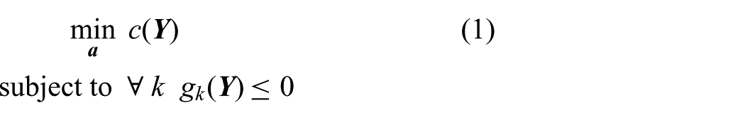
where, c is the cost function to be evaluated, and
The above optimization problem is usually computationally expensive. To increase the computational speed, efficient optimization techniques often require analytical gradient computation of the cost function and each constraint. The gradient can be decomposed as follows
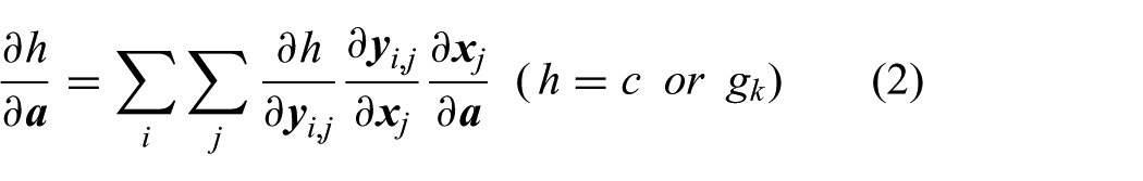
The gradient
First, the formulation should be extended for spherical joints, a free-floating base, or perhaps other types of joints in order to be applied to anthropomorphic systems because the formulations are originally for manipulators composed of rotational or translational actuators only. Though spherical joints or a free-floating base can be modeled by multiple rotational or translational joints, it often leads to the singularity problem of representing joint orientations. The link mass properties also need to be assigned to the corresponding multiple joints, which requires additional constraints on inertial properties and makes it difficult to perform dynamics analysis such as identification. The second issue is the computational complexity of the computation. The formulations in Suleiman et al. (2008) basically utilize the classical recursive formula of forward kinematics and inverse dynamics (Luh et al., 1980). The derivatives with respect to the coordinates of one joint are computed according to the recursive formula, and the same procedure is applied for every set of joint coordinates. Therefore, when computing the partial derivative of the variables of one link, the computational complexity is almost O (
In the field of computer animation, a similar framework of motion optimization has been applied to generate the motion of a human figure. Fang and Pollard (2003) presented an efficient method to compute the Jacobian of the total force and moment acting on the whole body with computational complexity O (
As mentioned above, one typical example of
The direct computation of Jacobian matrices does not always lead to the fast optimization. The gradient computation of h can be accelerated by avoiding the direct computation of Jacobian matrices, as seen in an efficient inverse kinematics computation for large-DOF system (Ayusawa and Nakamura, 2012). The computational speed is improved by decomposing the gradient computation into the combination of the forward kinematics and inverse dynamics computation. An efficient computation of the gradient inspired by such a method is introduced insection 5.
3. Mathematical notations and comprehensive motion transformation matrix
This section presents the preliminary notation of variables in the paper, and introduces a useful matrix to represent the forward kinematics computation including velocities and accelerations of the multi-body system.
3.1. Definitions of basic geometric and mechanical variables
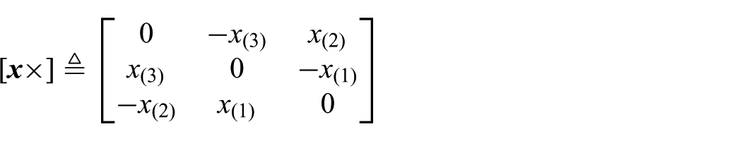
The skew operator is represented as follows
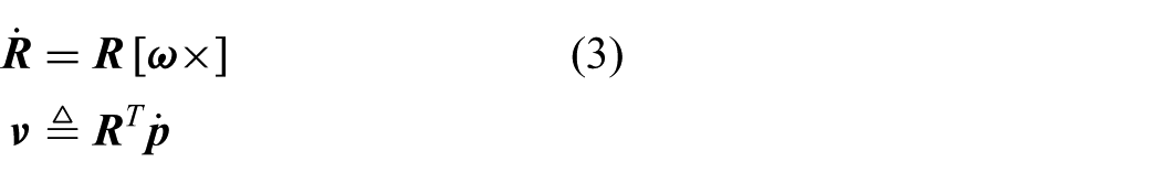
The position and orientation matrix of the coordinate system of a rigid body are
Let
The linear and angular velocities are concatenated and defined as in the following vector of spatial velocity
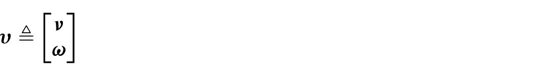
The
Let us define the operator for the linear and angular velocities as follows
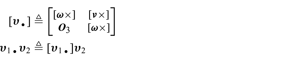
The above operator satisfies the binary operation axioms in Appendix A.1. The following important relationships also hold


The inertial properties of a rigid body consist of mass
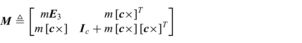
Let the inertial forces of a rigid body be
The equations of motion of a rigid body are

A variation of the above equation is written as follows by using matrix
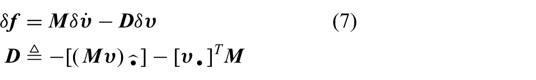
Operation
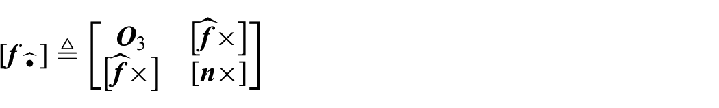
Note that the following relationship between [∙] and

3.2. Comprehensive motion transformation matrix (CMTM)
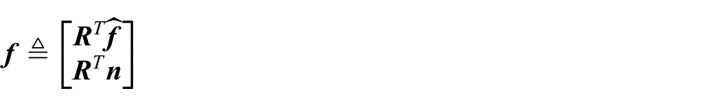
Let us define the following new
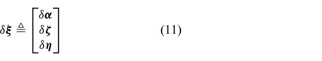
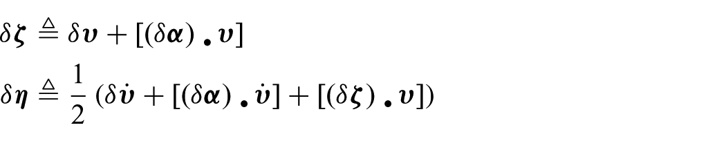
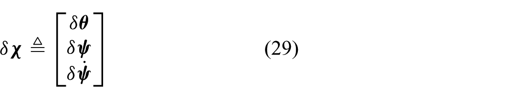
The following variation of the 18-dimensional vector is defined as follows
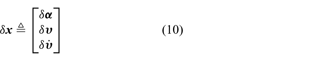
where variation

Vector
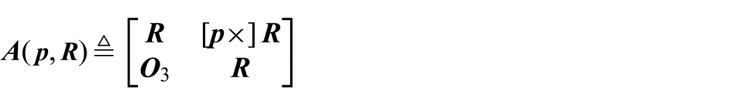
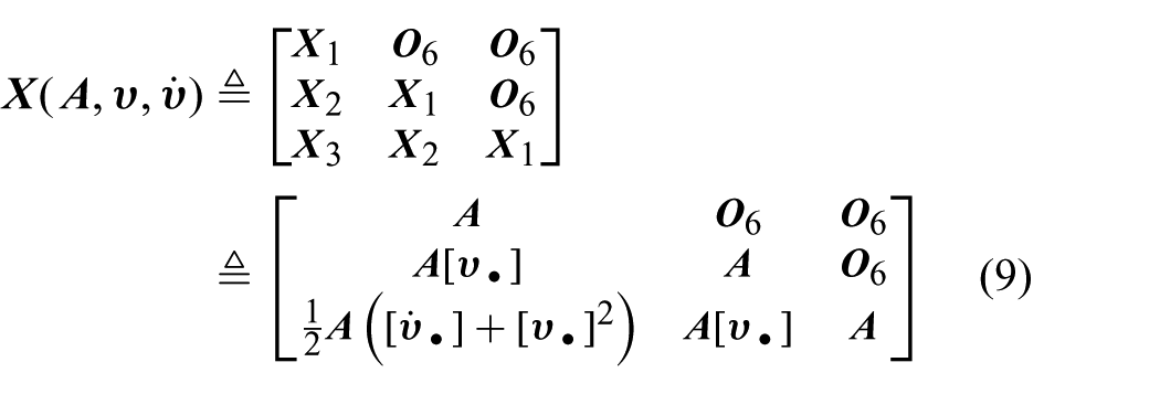
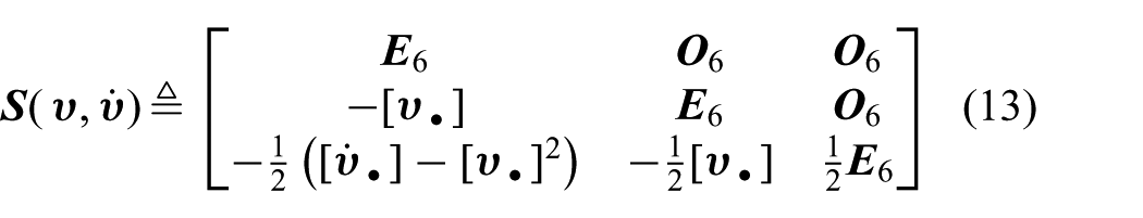
To handle the differential operation of matrix
where
For clarity, we summarize the above equations as follows

Matrix
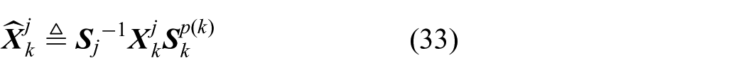
The inverse matrix of
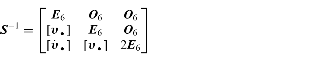
Although the variation
Let us now define the following matrix and operator
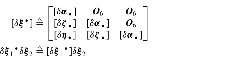
By utilizing the above operator, the following relationship holds

It can be verified by computing each block matrix of
Equation (14) has the same form as Equation (3) or Equation (4). Actually, operator

Note that Equation (15) corresponds with Equation (5).
The set of matrix
3.3. Definition and formulas of kinematics chain
This subsection presents the notation for open kinematic chain, and important formulas for the kinematics and dynamics.
The kinematic chain is tree-structured, and the indices are chosen from the base link toward the end of branches.
Let us define the following sets
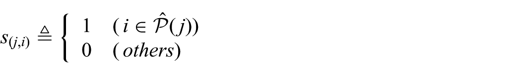
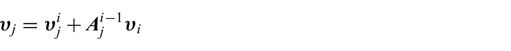
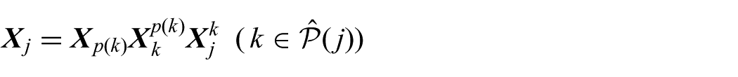
Let us represent the quantity
Let us denote

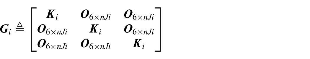
Matrix
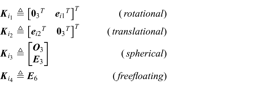
where
Vector
Note that, in the case of spherical joints or free floating joints, the tangent vector
Vector

Vector
where
Vector
3.4. CMTMs in the kinematic chain
Let us consider the following chain product of CMTMs

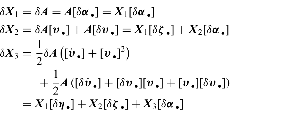
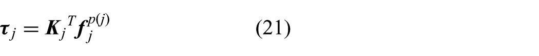
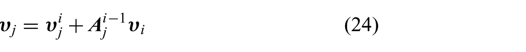
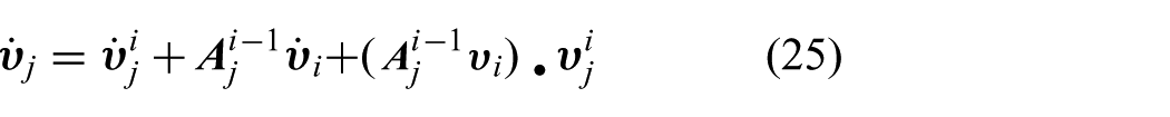
The chain products of CMTMs in Equation (22) represent the forward kinematics computation including differential kinematics for the velocity and acceleration as follows

The above relationships can be easily verified by writing the components of


Now let us examine Equation (26), Equation (27), and Equation (28). From Equation (9), Equation (26) can be transformed into

Therefore, Equation (26) is equivalent to Equation (23): the standard forward kinematics operation.
Next, Equation (27) can be converted into
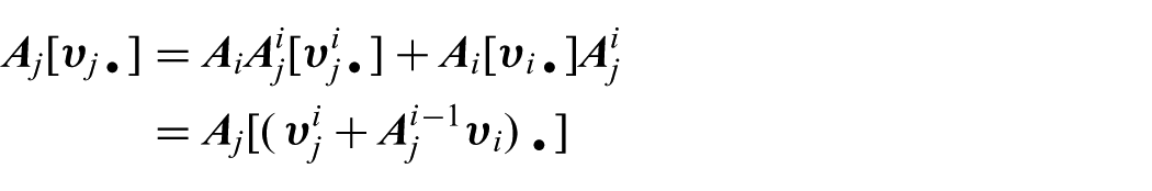
From the above equation, the following must also hold
Therefore, Equation (27) is equal to Equation (24), i.e. the differential forward kinematics operation about linear and angular velocities.
Finally, Equation (28) can be written as follows
Therefore, the following must hold
Then, Equation (28) is transformed into Equation (25), i.e. the differential forward kinematics operation for the linear and angular accelerations.
□
From the above, it is apparent that the chain products of CMTMs in Equation (22) represent the standard and differential kinematics computation of a kinematic chain. The formulation using CMTM can therefore handle the kinematics operations in a comprehensive manner. This is a strong advantage when introducing arbitrary Jacobian matrices in the next section.
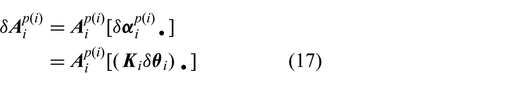
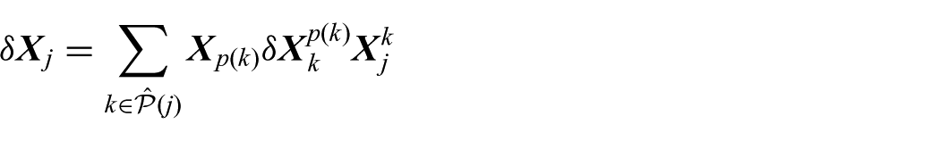
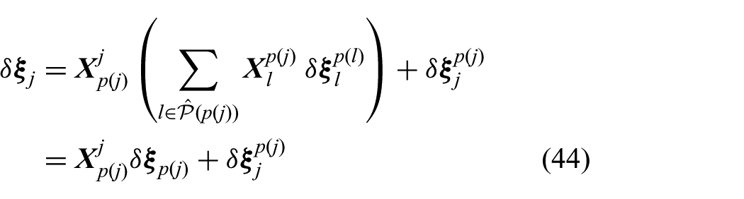
Now let us define the following variation of
According to Equation (11), Equation (17), and Equation (18), the relationship between

where
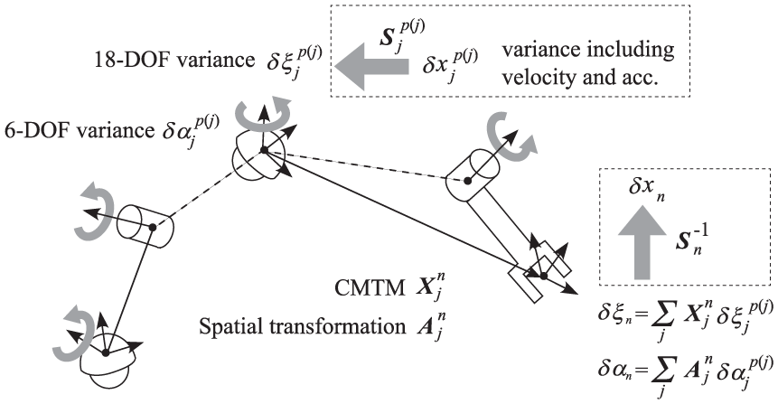
The relationships between the variables of the link and joint coordinates and their variations are summarized in Figure 1.
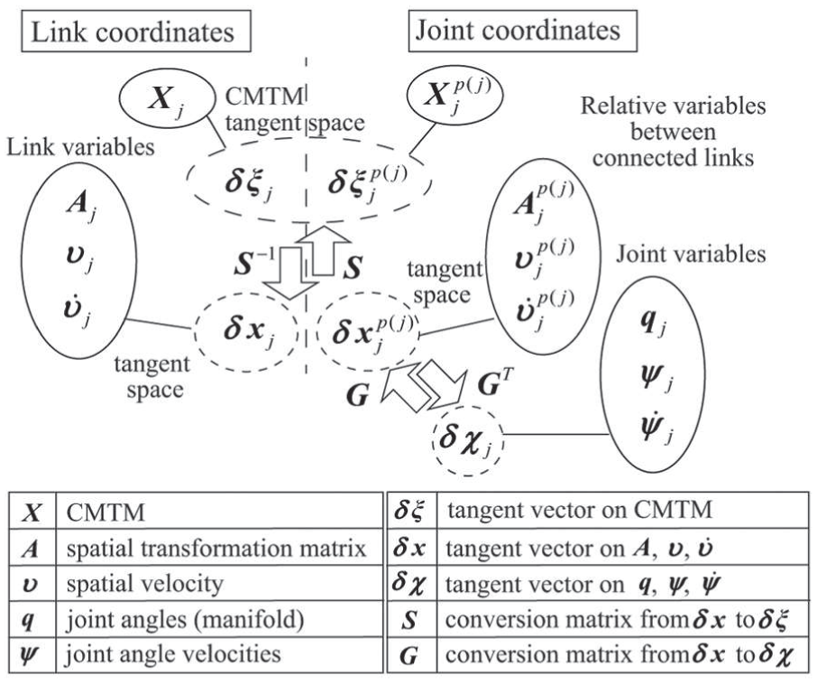
Overview of the relationships between the variables used in the paper.
4. Computation of arbitrary Jacobians
This section shows the different types of arbitrary Jacobian matrices used in Equation (2) by utilizing CMTM. The formulation in this paper are strictly speaking not Jacobian matrices as in the case of the basic Jacobian. The basic Jacobian is the coefficient matrix in the linear differential relationship between the joint angle velocities and the linear/angular velocities of the corresponding link. Since the integration of angular velocity has no physical meaning, the corresponding part of the basic Jacobian is not equivalent to the partial derivatives of the orientation variable. Several Jacobians introduced in this section also mean the coefficient matrices in the linear differential relationship between the variation of joint variables
4.1. Jacobians of link posture, velocity and acceleration
Let us compute matrix
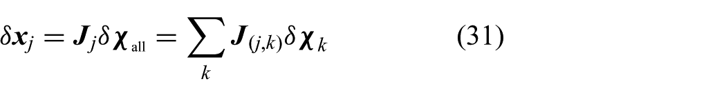
where,
The matrix
where
This subsection contains the proof that Equation (32) holds. The Jacobian
The relationship between basic Jacobian and the variance defined with CMTM. The new framework can also be applied to free-floating and spherical joints.
As mentioned in the previous section, matrix
Let us consider
Then, the variation of
By utilizing Equation (14) and Equation (15), the above equation can be transformed into
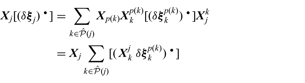
According to the above equation, the following equation also holds
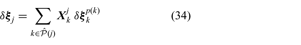
The coefficient matrix of Equation (34) represents the Jacobian matrix with respect to
Because the desired Jacobian matrix is with respect to
First, by utilizing Equation (12), the following equation is obtained
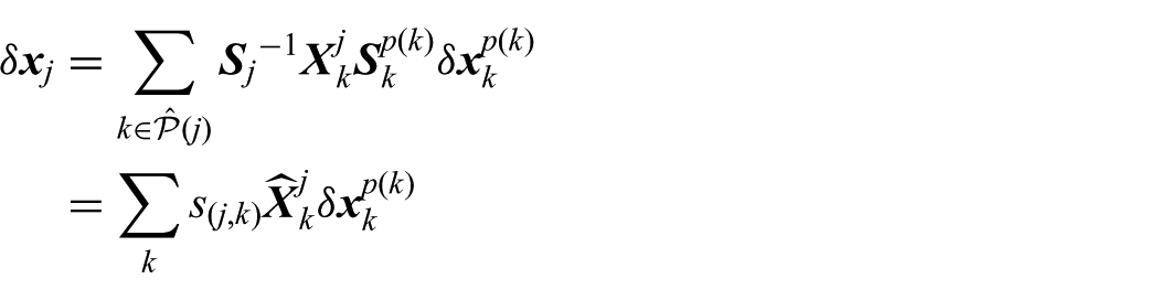
The next transformation can be performed with Equation (30) as follows
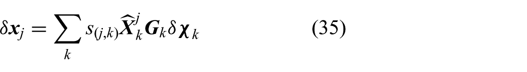
From Equation (35), the Jacobian matrix shown in Equation (31) was finally derived as given in Equation (32).
□
The computation of
4.2. Jacobians of link inertial forces
This subsection derives matrix
where,
The matrix

where

This subsection verifies Equation (37).
Let us first consider the variation of equations of motion of link j. According to Equation (7), the following equations are obtained

From Equation (31), the above equation can be also transformed into the following
Therefore, the Jacobian matrix shown in Equation (36) could be derived as Equation (37).
□
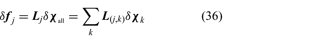
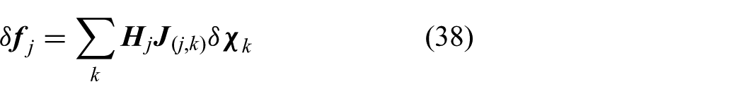
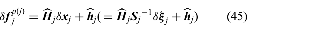
For the sake of the subsequent discussions, let us transform Equation (38) to a linear form with respect to
4.3. Jacobians of joint constraint forces
In this subsection, we compute matrix
where,
The matrix
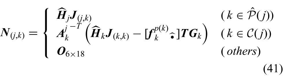
where, matrix
Additionally, matrix

Let us verify Equation (41) in this subsection.
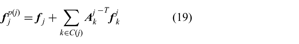
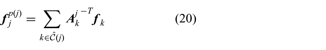
From Equation (19), the following equation about the joint constraint force
According to Equation (39), the above equation can be transformed into
On the other hand, the following equation holds from Equation (34)
Because
where
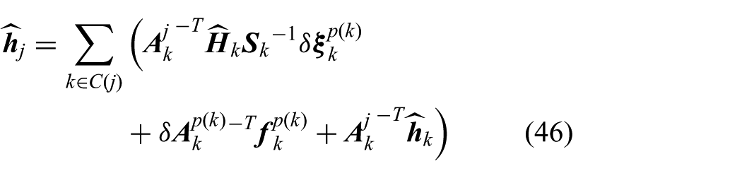
It should be noted that, if the set of
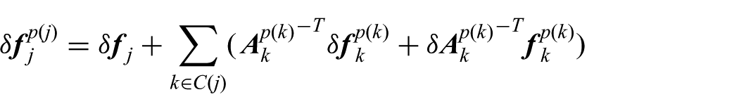
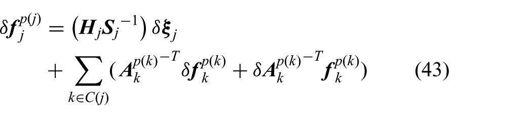
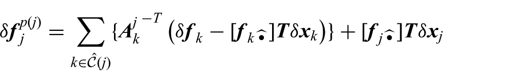
Let us expand the term of
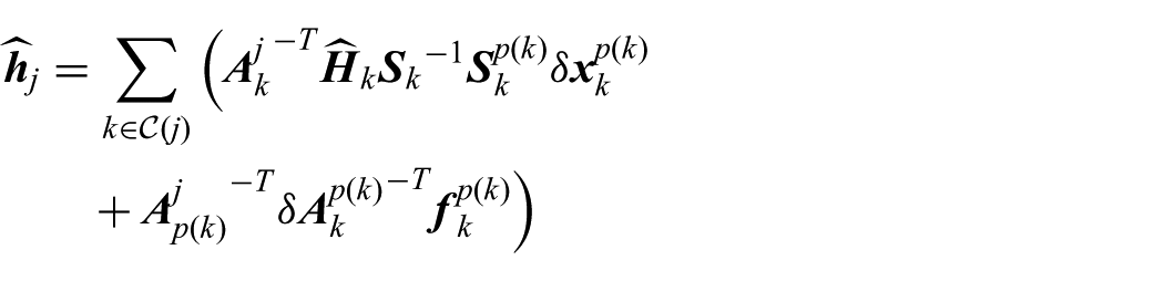
There also exists the following conversion of variation
According to the above equation,
Note that,
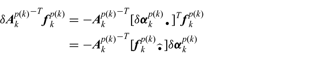
By substituting Equation (42) and Equation (47) for Equation (45), and by converting the variations from
From Equation (48), the Jacobian matrix shown in Equation (40) can be finally derived as given in Equation (41).
□
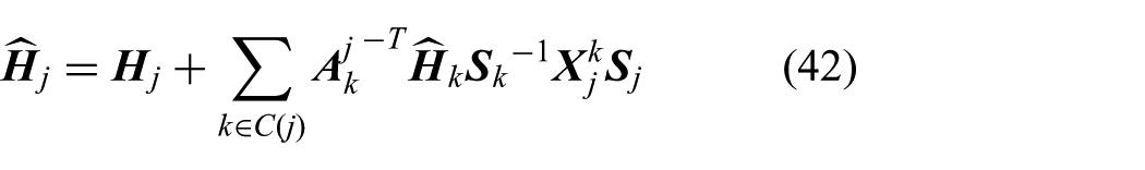
The important advancement from the conventional formulation (Suleiman et al., 2008) is the recursive formula of inertial matrices in Equation (42), which achieves significant improvement in computational efficiency. The computation of Equation (41) requires matrix
The direct computation of Equation (42) with
4.4. Jacobians of joint torques
Let us compute matrix
where,
The variance of the joint torque
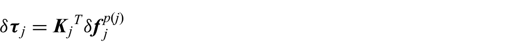
Therefore,

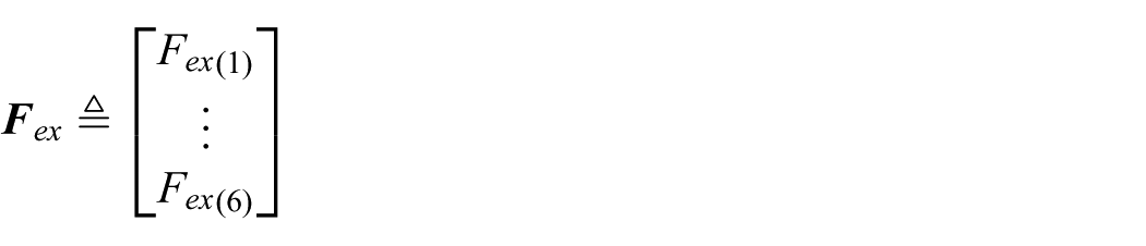
4.5. An application: Jacobian of ZMP
Since ZMP is often used for the analysis of the balancing problem of humanoid systems, its Jacobian matrix will be useful in the motion optimization framework. This subsection presents the method of computing the Jacobian matrix of ZMP.
The total external forces acting on the kinematic chain are equivalent to
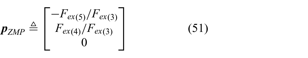
where
Let us compute matrix
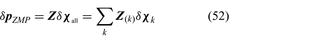
where,
The variance of Equation (51) can be formulated as follows

where
Therefore, the Jacobian

5. Advanced implementation with decomposed gradient computation
Let us consider the following function
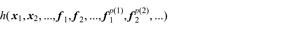
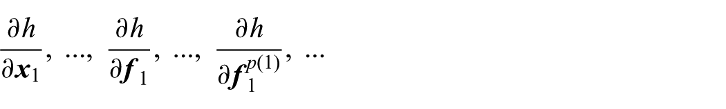
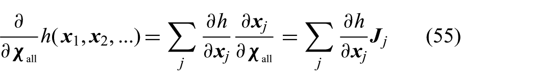
This function corresponds to the cost function or the each function of the corresponding constraint in Equation (1). The function contains several physical quantities such as link coordinates, link inertial forces, joint forces, etc. The gradient of the function with respect to each physical quantities is as follows
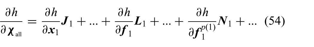
When solving the optimization problem such as Equation (1), the gradient of the function with respect to the joint variables
In many cases, the cost function or each constraint function has a simple structure with respect to each physical quantity. A typical example for cost functions is the summation of the quadratic form of each physical quantity such as
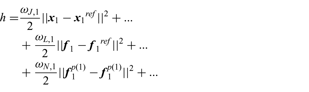
where,
This section introduces an efficient computation method of Equation (54) with computational complexity O
5.1. Gradient computation of arbitrary functions of
Let us consider an arbitrary function
The simple formulation when computing
This subsection introduces an efficient method of computing Equation (55).
The first step computes the gradient
By using Equation (34), we can further have
The above summation formulas can be transformed into the recursive formula as follows
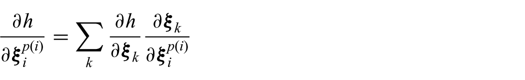
Next, let us convert the variable
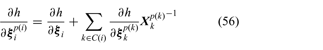
By using the above relationships, Equation (56) can be transformed into the following
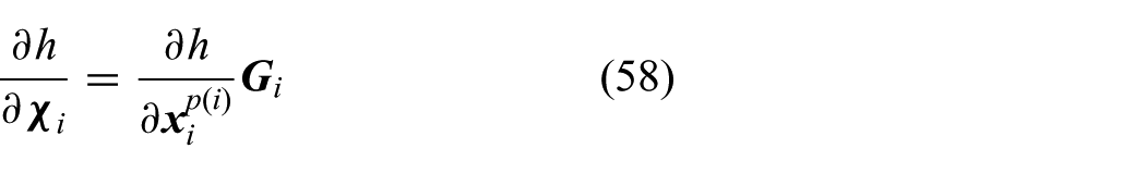
Further, from Equation (33) we have
Equation (57) indicates that, if the gradient
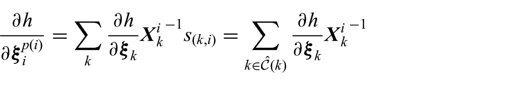
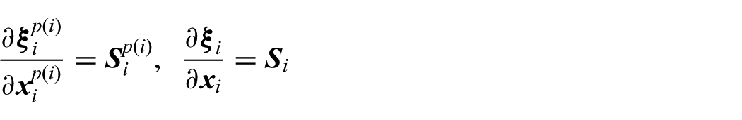
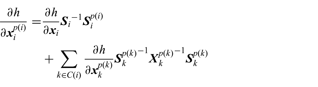
Finally, let us convert the variable
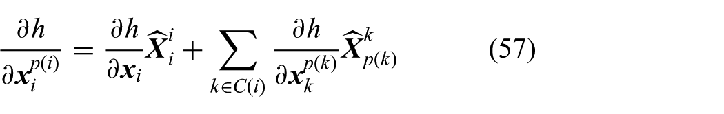
By using the above equation, Equation (57) can be transformed into
From the above formulations, the computation of Equation (55) can be archived by the following computations.
Compute Equation (57) recursively from the end-links.
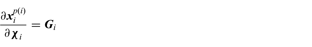
Compute Equation (58).
The complexity of the decomposed gradient computation introduced in this subsection is
5.2. Gradient computation of arbitrary functions of
Let us consider an arbitrary function
The simple formulation when computing
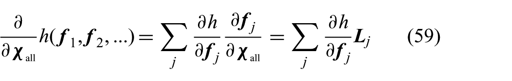
This subsection presents a method of computing Equation (59).
First, let us consider the gradient
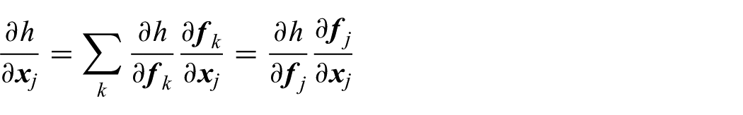
From Equation (38), we can have
Finally, the above equations can be transformed into
Since Equation (60) provides
5.3. Gradient computation of arbitrary functions of
Let us consider an arbitrary function
The simple formulation when computing
This subsection introduces its efficient computation.
First, let us formulate the variation of
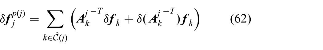
The matrix variation
Therefore, the term
By substituting
By using this relationship, Equation (62) can be transformed into
By substituting Equation (40) and
Then, the following partial derivative holds
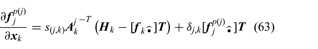
where,
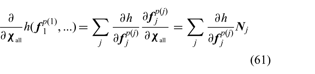
Next, let us compute the gradient
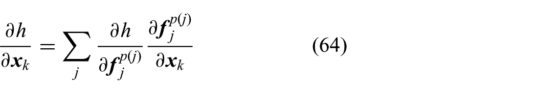
By substituting Equation (63) into the above, the gradient can be computed as follows
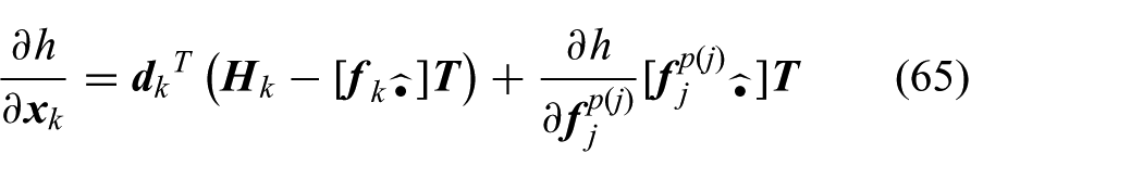
where
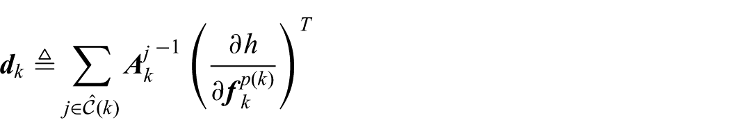
The vector
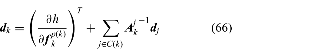
Finally, the gradient
Compute Equation (66) for all k from the end-links.
Compute Equation (65) for all k.
Since
5.4. Gradient computation of other functions
The joint torque
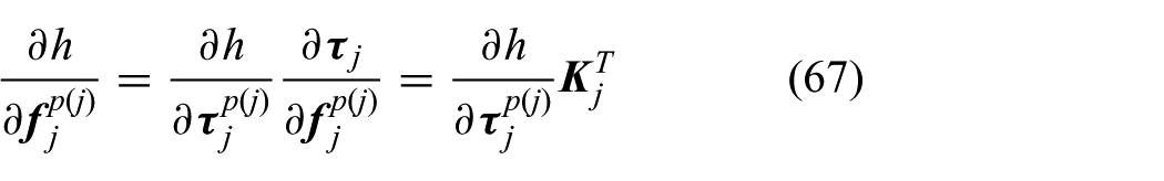
When the function contains the joint torque
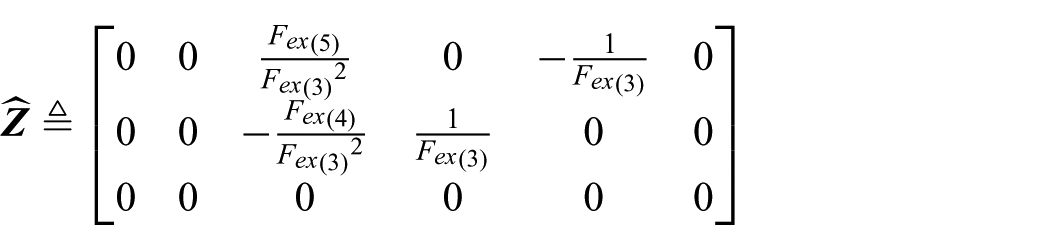
Similar to the case of the joint torque, ZMP
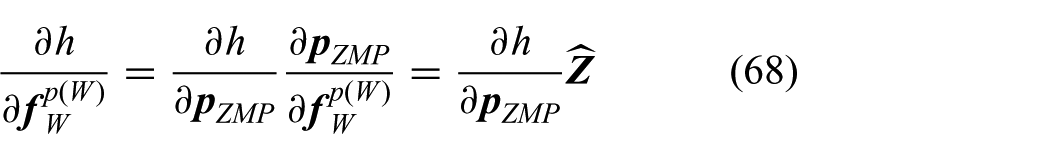
When the function contains
6. Numerical evaluation
6.1. Comparison of computation time of Jacobian matrices
We here show the comparison of the computation times of the Jacobian matrices for the three approaches: the proposed method shown in Section 4, the traditional method in Suleiman et al. (2008), and the automatic differentiation method. Since the formulations in Suleiman et al. (2008) only handle 1-DOF joints, it was tested by using a serial manipulator with N rotational joints. The Jacobian matrix of the joint torque of the first rotational joint was computed by changing the number of joints. We implemented the automatic differentiation of the joint torque computation by using Adept (Hogan, 2014): a combined automatic differentiation and array library for C++. The methods were tested on the computer with Intel(R) Xeon(R) CPU E3-1535M v5. The proposed method generated the same Jacobian matrices as those from the other two methods. Figure 3 shows the results of the computational time of the two methods, demonstrating its correctness.
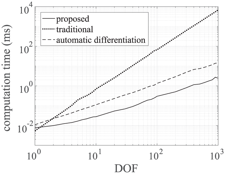
Comparison of computation time of joint torque Jacobian matrix.
The computational complexity of the conventional method was
6.2. Comparison of computation time of gradient
This subsection evaluates the performance of the proposed method of computing the gradient of the cost function. We tested the method by using the same serial manipulator model used in the previous subsection. The following two cases were considered.
The cost function contains the joint torque of only one joint:
The cost function contains the joint torque for all joints:
We computed
The comparison of computation times in case (A) is shown in Figure 4, and that in case (B) is in Figure 5. The solid lines represent the computation time with DGC, and the dotted lines indicate the time without DGC. The gradient computation without DGC in case (A) requires the Jacobian matrix of the joint torque of only one joint. This leads that the computational complexity without DGC is also O(
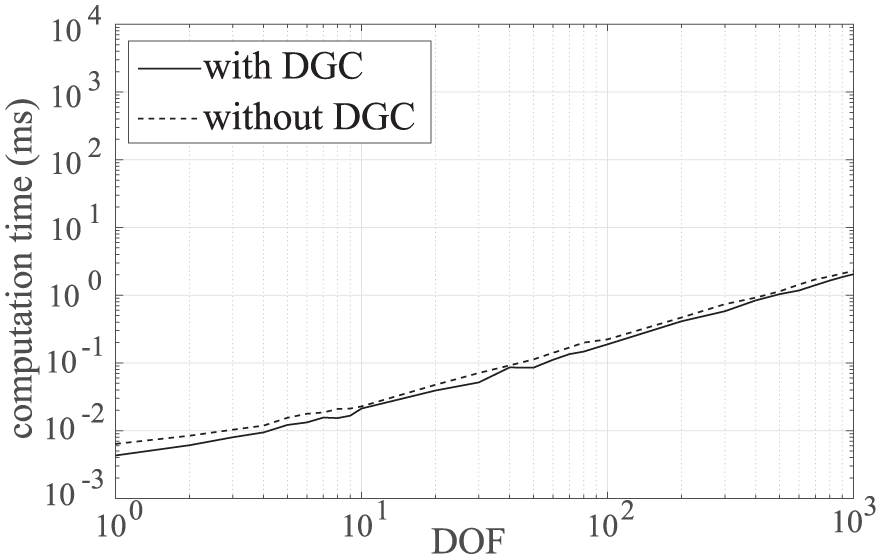
Comparison of computation time for gradient computation when the number of constraint is 1. The solid line (with DGC) represents the time with the proposed decomposed gradient computation. The dotted line (without DGC) indicates the time without the decomposed gradient computation and with computing the Jacobian matrices.
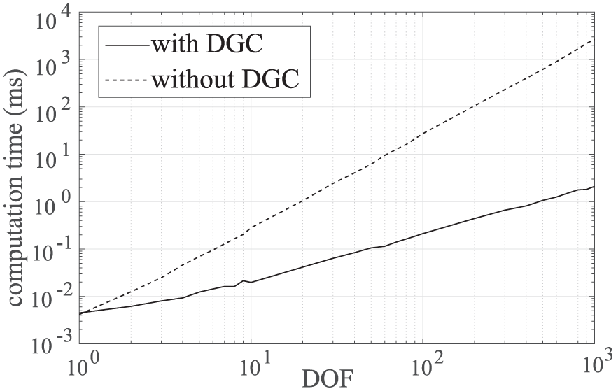
Comparison of computation time for gradient computation when the number of constraint is
6.3. Motion optimization of spherical joint manipulator
The proposed method is applied to a redundant serial robot manipulator composed of five spherical joints, in order to validate the Jacobian for the case of spherical joints. The 15-DOF manipulator moved in a complex environment cluttered with non-convex obstacles and no gravity. Each link featured the following physical quantities: for link i,
In this trajectory optimization, the total time length of the trajectory was assumed to be 2 s, and its sampling rate was 5 ms. The variables of the spherical joints were represented by an angle-axis vector, and their trajectories were modeled using B-splines, as shown in Suleiman et al. (2008). The number of B-spline bases was 24, and the timespan between the two bases was 0.1 s. The position of the end-effector started from
All the constraint conditions were converted to penalty cost functions according to the penalty function method
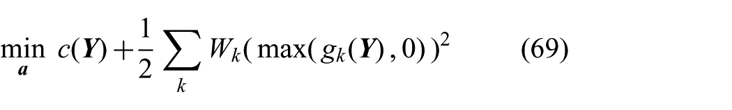
where,
The generated trajectory is shown in Figure 6. The end-effector successfully passed through the targeted positions without colliding with any obstacles. The results of the joint torque trajectories for the first joint are shown in Figure 7, and they all satisfy the joint torque limitations. The other joint torques also satisfied the limitations as shown in Figure 8.
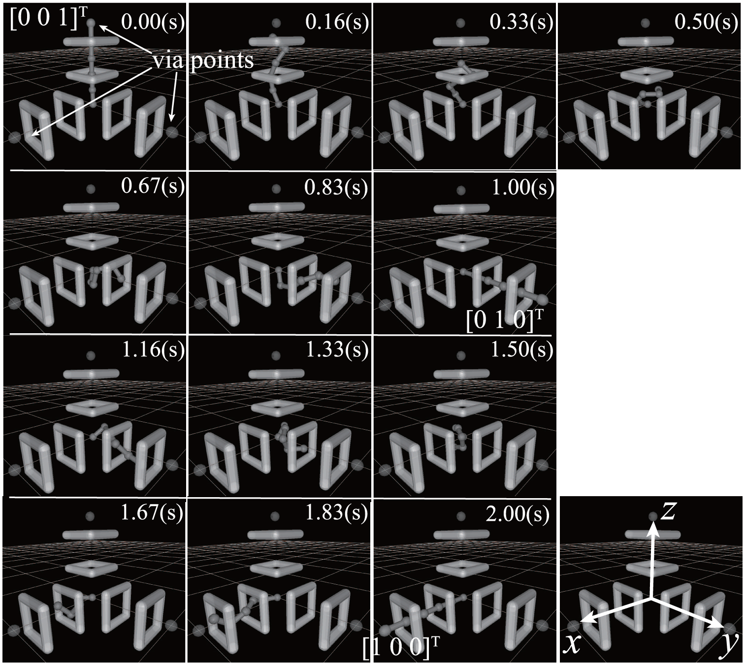
Snapshots of the generated motion of the redundant robot in a cluttered environment. Starting from the initial position
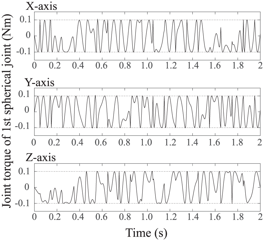
Resultant joint torque trajectories of the base spherical joint. The torque limit of small value of
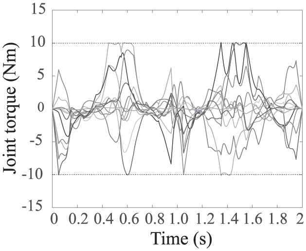
Resultant joint torque trajectories of all the joints except for the base joint. All the 12 lines are within the torque limit of
6.4. Motion optimization of humanoid robot
As one of the practical applications where the proposed framework is useful, this subsection shows an example of the motion optimization for dynamic parameter identification of a humanoid robot (Ayusawa et al., 2017).
The optimal trajectory for dynamic parameter identification is called the persistent exciting (PE) trajectory (Gautier and Khalil, 1992). To generate the PE trajectory, the condition number of the “regressor matrix” obtained from the joint trajectory should be minimized while maintaining dynamic constraints. Although we showed an analytical framework to optimize the condition number in our previous work (Ayusawa et al., 2017), the stability was considered only statically by using the center of mass (CoM), which is conservative and may limit the identification performance. In the resultant motions, both feet were placed to the ground because the dynamic stability condition became too severe to be satisfied only by the CoM condition. This limitation makes it difficult to generate dynamic leg motions by standing on one leg for better identification. In the proposed framework, the analytical computation of the Jacobian of the ZMP can be provided, which can guarantee the dynamic stability constraint in the trajectory optimization.
We have derived a dynamically stable optimal PE trajectory on one leg by constraining the ZMP inside the area of 4 cm and 1 cm around the center of the standing foot in front and lateral direction. The trajectory is parameterized by B-Spline using physical properties from the robot CAD model. We also added constraints on forces and torque applied on the ankle so that the horizontal forces
As shown in the snapshots in Figure 9, the humanoid HRP-4 (Kaneko et al., 2011) successfully performed the optimized PE trajectory on dynamic simulator Choreonoid (Nakaoka, 2012), which validates the feasibility. The total computation time without DGC was 12826 s. DGC accelerated the optimization so that its computation time was 2857 s. The result of the optimized condition number was 124.2, small enough to indicate that a dynamically stable optimal trajectory for dynamics identification of the robot were generated successfully by using the proposed framework.
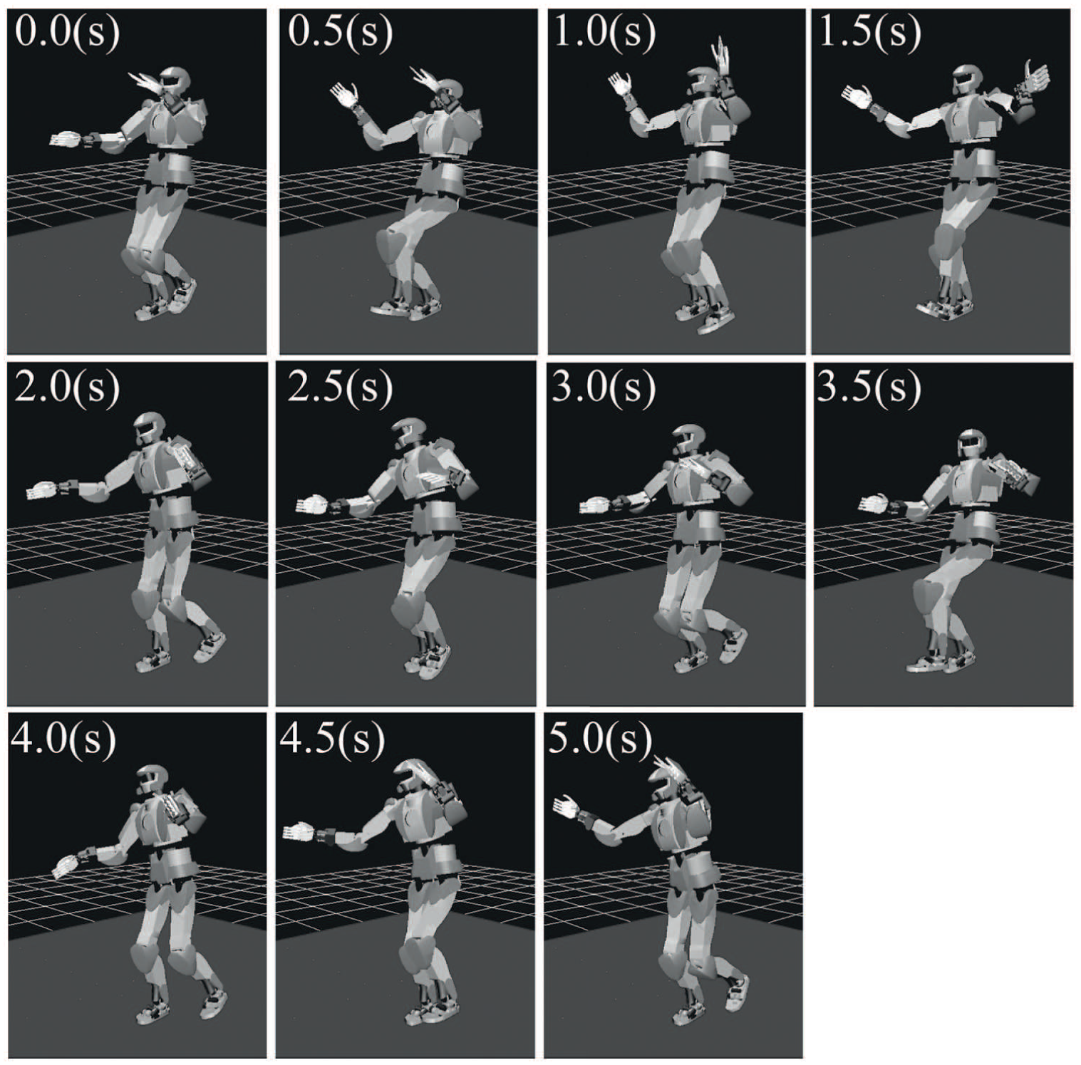
Snapshots of optimized one-leg PE trajectory for dynamic parameter identification. The humanoid robot HRP-4 can successfully perform resultant whole-body motion by also exciting the free leg.
7. Conclusion
This paper presented a comprehensive theory of differential kinematics and dynamics to derive analytical partial derivatives of both link/joint quantities with respect to joint coordinates and their derivatives. First, the 18×18 comprehensive motion transformation matrix (CMTM) and 18-dimensional product operation was introduced for comprehensive kinematics formulation, which allows a simple chain product of the matrices to represent the differential forward kinematics of a kinematics chain. They also have the same features as the rotation matrix and the 6×6 transformation matrix, and their product operations. By utilizing CMTM, the partial derivative of the link coordinates and their derivatives were derived in the same manner as when introducing the basic Jacobians by just replacing the 6×6 transformation matrices with CMTM in their formulations.
This novel theoretical framework added the following contributions to current work. The partial derivatives of each generalized force with respect to the joint coordinates and their derivatives were also demonstrated. The derivation procedure also has a similarity to that of the linear and angular momentum Jacobians. The formulation can also handle different types of joints such as spherical joints or free-floating bases. We have also shown that the analytical derivative of physical quantities like ZMP can be easily computed with the proposed method, which is an important advantage for practical human/humanoid motion optimization. By utilizing the CMTM, each new Jacobian could be computed with O(
The optimization problem often can be solved efficiently by avoiding the direct computation of Jacobian matrices, as indicated in Ayusawa and Nakamura (2012). The fast gradient computation algorithms were also proposed to lead to more practical implementation. Evaluation of cost function composed of different types of physical quantities usually requires a heavy computational cost. Together with the decomposed gradient computation method (Ayusawa and Nakamura, 2012), the gradient computation could be performed with computational complexity O(
A couple of application examples were presented to demonstrate the usefulness of the proposed framework. We showed the dynamic trajectory optimization of a redundant serial robot manipulator composed of spherical joints. A collision-free dynamic motion was successfully generated in a cluttered environment with non-convex obstacles, while simultaneously imposing a strong torque limit. This validates the basic trajectory optimization capacity of the proposed framework under severe constraints. Another application is optimization of the PE trajectory for identification of dynamic parameters of a humanoid robot. In this example, the analytical gradient of ZMP with respect to joint angle and its derivatives was utilized to guarantee the balance. Dynamic one-leg PE motions were generated and their validity was confirmed via a dynamic simulator.
The mathematical features of CMTM and its operator have a similarity to those of the rotational matrix and the cross product or those of the spatial transformation matrix and the screw operation. The rotational or screw motion of a rigid body has been studied from the view point of a Lie group and Lie algebra. Future work will focus on the features of CMTM from that point of view.
This paper represented the trajectory variables in the motion optimization of the joint coordinates and introduced the Jacobian of forces with respect to the joint coordinates according to the inverse dynamics formula. Concerning control issues, we often consider the joint torques as controller input variables and optimize them. Though the Jacobian with respect to the joint torques can be obtained by computing the inverse matrices, there is another possibility of inverse Jacobian formulation according to the efficient formula used in forward dynamics computation (Featherstone, 1983), which will be addressed in our future work.
There is still room for improvement in computation time of the proposed method by using parallel computation for multi-body systems (Featherstone, 2008). An algorithm for parallel computation will be investigated for future applications such as the real-time control of a humanoid robots or the motion analysis for a complicated human skeletal system.