Instantaneous Kinematics Analysis via Screw-Theory of a Novel 3- C RC Parallel Mechanism

Abstract

This paper presents the mobility and kinematics analysis of a novel parallel mechanism that is composed by one base, one platform and three identical limbs with CRC joints. The paper obtains closed-form solutions to the direct and inverse kinematics problems, and determines the mobility of the mechanism and instantaneous kinematics by applying screw theory. The obtained results show that this parallel robot is part of the family 2R1T, since the platform shows 3 DOF, i.e.: one translation perpendicular to the base and two rotations about skew axes. In order to calculate the direct instantaneous kinematics, this paper introduces the vector m_h, which is part of the joint velocity vector that multiplies the overall inverse Jacobian matrix. This paper compares the results between simulations and numerical examples using Mathematica and SolidWorks in order to prove the accuracy of the analytical results.

1. Introduction

Parallel mechanisms (PMs) have been intensively studied for several years by the academic community due to their high complexity and potential applications. A PM is composed of a moving platform that is connected to the base by at least two serial kinematic chains in parallel that constrain the platform, resulting in a multi degree-of-freedom (henceforth denoted as DOF) mechanical system[1]. PMs have evolved from geometric shapes to complex mechanisms. One of the early implementations of PMs is found at St. Paul's Cathedral in London, where Christopher Wren included parallel towers and a triple dome design in order to improve the load capability of the structure [2]. In 1813, the French mathematician Augustine Louis Cauchy studied regular and irregular polygons and polyhedrons, resulting in the “ articulated octahedron”, a parallel structure that serves as a predecessor to the hexapod [3]. This work was further studied by Lebesgue in 1867 [4] and led to the three types of flexible octahedra introduced in 1892 by Raoul Bricard [5].

PMs are well-known for showing features such as: (i) high accuracy; (ii) good load/weight ratio; (iii) higher structural stiffness compared to serial mechanisms. Furthermore, PMs are similar to truss structures, where all motors are commonly placed on the base, resulting in high accelerations of the end-effector. PMs have been subjected to diverse applications, e.g. the tire testing machine by Gough and Whitewall [6] and the moving platform for flight simulation built by Stewart [7]. One of the most successfully adopted PMs by the industry is the delta robot [8], which is commonly used for pick-and-place applications. In addition, PMs are used as haptic devices, for example, the spherical PM, which provides real-time motion and/or force feedback to the user in teleoperation tasks [9]. Another example is the parallel micro-robot, which is designed for manufacturing tasks where high precision and accuracy are needed [10]. Several kinematics analyses have been conducted in the literature to validate the feasibility of applying PMs for specific tasks; these analyses pertain to the challenges PMs face for being widely adopted in industry i.e. their (i) limited workspace and (ii) kinematic complexity. PMs can be classified according to the their mobility as: (i) full or (ii) lower mobility mechanisms. The platform of a full mobility PM experiences 6 DOF, whereas a lower mobility PM has less than 6 DOF and are also known as limited mobility PMs. Despite the loss of mobility and a degree of loss of flexibility, there is a tendency toward the study of this type of PM, since they can be used in more specific tasks.

This paper focuses on 2R1T manipulators that refer to platforms with 3 DOF, namely two rotations and one translation, which have recently gained interest in the scientific community. Rodriguez-Leal et al. [11] used screw theory to analyse a family of 2R1T PMs, which included the 3-PSP, 3-PPS, 3-PCU and 3-CUP PMs (where C denotes cylindrical joint, R denotes revolute joint, P denotes prismatic joint, S denotes spherical joint and the underline indicates that the joint is actuated). Another example of work conducted with 2R1T PMs is the 3-PSP architecture studied by Di Gregorio et al. [12]. A study of the mobility, direct and inverse positioning and instantaneous kinematic analysis of PMs was performed in [13]. The above mentioned examples of PMs have been proposed in order to produce lower mobility PMs that have lower cost than full mobility PMs, and that are applied in specific tasks where full mobility PMs are overqualified for the same tasks. The novel architecture presented in this paper was developed through the mechanical modification of the 3-CUP PM presented in [13, 14] and [15] in order to simplify the construction of a PM that has the features of the 2R1T family.

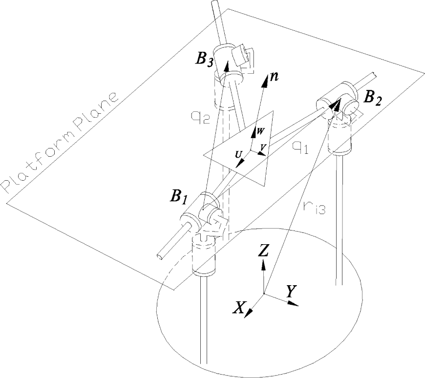
This paper focuses on the analysis of the novel 3-CRC PM architecture that is composed of a base that is connected to a moving platform by three identical CRC limbs; these are a C joint, which is formed by an actuated P joint whose axis is collinear to a passive R joint and consecutively connected to passive R and C joints. For the convenience of the reader, a CAD model of the 3-CRC manipulator is shown in Fig. 1. Since the mechanism is classified as a 2R1T PM, its platform exhibits 3 DOF, i.e. two rotations about skew axes and a translation on the perpendicular axis to the base.

Figure 1.

The 3-CRC Parallel Robot

This paper presents a complete mobility and kinematic analysis of the 3-CRC PM. For the mobility analysis, this paper follows the screw theory-based method proposed by Dai et al. [16] in order to obtain precise insight into the type of DOFs shown by the platform under analysis. The kinematic problem is solved by investigating the loop-closure equation of the PM, which results in a closed-form solution of the inverse kinematics problem [17].

One of the fundamental theoretical problems of PMs is instantaneous kinematics, which is addressed by using the theory of reciprocal screws and applying the methodology presented by Joshi and Tsai in [18] in order to obtain the Jacobian matrix, which relates the joint and end-effector velocity. A novel application of this 3-CRC PM can be in metal additive manufacturing, where the PM acts as a base and a serial robot includes a torch that deposits the material on the PM platform. Another application for the 3-CRC is the manipulation of any large object or structure in a given manufacturing process, e.g. the airplane fuselage assemble process.

This paper is arranged as follows: section 2 introduces the notation used in this study and describes the topology of the parallel manipulator. Section 3 presents a mobility analysis of the mechanism via screw theory. The solution to the direct and inverse kinematics problem via the analysis of the loop-closure equation is contained in section 4. In section 5, the Jacobian matrix is obtained by applying the methodology developed by Joshi and Tsai in [18]. Furthermore, numerical examples and simulations included in section 4 and 5 that were performed using commercial software such as Mathematica and Solidworks validate the mathematical models presented in this paper. Finally, section 6 presents conclusions and future proposed research on this 3-CRC PM.

2. Manipulator Description

It is well-known in the literature that PMs are named according to the number of limbs and type of joints contained in the kinematic chain formed by each limb. Hence, 3-CRC is a PM constructed of three identical and equally distributed limbs that connects the base to the moving platform. A schematic diagram of a CRC kinematic chain is shown in Fig. 2.

Figure 2.

Screw-joint schematic of limb i of the 3-CRC (3-PRRRP) PM

The scalar quantities are represented in this paper by lower case lettering in italic type (e.g., a), vectors by lower case lettering in bold italic type (e.g., $d_i$ ) and matrices by upper case lettering in bold upright type (e.g., $R$ ). Cartesian coordinate reference frames and their orthogonal axes are denoted by upper case lettering in italic type (e.g., G). Centroids and fixed points in links are denoted by upper case lettering (e.g., C). Furthermore, consider S, C and T as abbreviations of sine, cosine and tangent, respectively.

In order to investigate the mobility of the manipulator and describe the position and orientation of the platform relative to the base, two frames will be defined. Consider the first global frame in Fig. 2 with its origin at the centroid O of the fixed base, to be denoted as $G(X\mathrm{,}Y\mathrm{,}Z)$ . The second frame is attached to the moving platform with an origin at the centroid C and is denoted as $H(U\mathrm{,}V\mathrm{,}W)$ . Vector $p$ describes the position of C in the three-dimensional space referred to as the global frame G. The subscript $ij$ denotes the joint $j\left(=\mathrm{1,2,3,4,5}\right)$ on leg $i\left(=\mathrm{1,2,3}\right)$ ; consider now that vector $s_{ij}$ represent the axis of joint $ij$ . Note that the C joints are conformed by the P and R joints, whose axes are coaxial and where the CRC kinematic chain is equivalent to a combination of PRRRP joints. The P joint connected to the base is denoted as $j_{i1}$ , the next R joint is denoted as $j_{i2}$ , the following R joint is denoted as $j_{i3}$ and the C joint that lies on the moving platform is denoted as $j_{i4}$ and $j_{i5}$ for the R and P joints, respectively. The limbs of the PM are equally distributed by an angular position given by the angle ψ_i, which is a rotation about the Z -axis ( ${\psi }_1=0°\mathrm{,}{\psi }_2=120°$ and ${\psi }_3=240°$ ), and located on the $XY$ plane by the vector $a_i$ , where a is the magnitude and represents the distance from O to point ${\mathrm{A}}_i$ , while the magnitude of vector $d_i$ is d and represents the stroke of joint $j_{i1}$ , whose joint axis $s_{i1}$ is perpendicular to the base and describes the distance between point ${\mathrm{A}}_i$ and ${\mathrm{B}}_i$ . Furthermore, joint $j_{i2}$ represents a rotation about the axis $s_{i2}$ that is coaxial with $s_{i1}$ . As shown in Fig. 2, note that all the joint axes $s_{i1}$ , $s_{i2}$ , $s_{i3}$ , $s_{i4}$ and $s_{i5}$ intersect at point ${\mathrm{B}}_i$ . The C joints located on the moving platform are distributed by an angular position given by the angle χ_i, which is a rotation about the W -axis ( ${\chi }_1{=0}^{\circ }\mathrm{,}{\chi }_2{=120}^{\circ }$ and ${\chi }_3{=240}^{\circ }$ ), and their strokes are denoted by vector $b_i$ , whose joint axis is $s_{i5}$ and which lies on the $UV$ plane, and its rotation is about the axis $s_{i4}$ . Finally, the R joint described by axis $s_{i3}$ is constrained to be parallel to the $XY$ plane and is perpendicular to the axis $s_{i5}$ .

3. Mobility Analysis

This paper approaches the mobility analysis through the use of screw theory. Recall that according to the literature [19], a screw is commonly represented as:

$\$=\left[\begin{array}{c}{\left\{\begin{array}{c}s\end{array}\right\}}^T\\ {\left\{\begin{array}{c}r\times s+hs\end{array}\right\}}^T\end{array}\right]$

(1)

Where vector $s$ indicates the axis of $\$$ and vector $r$ is any vector drawn from any point of the axis of $ to the centroid of the Cartesian coordinate reference frame. Note that the velocity vector is obtained from the cross product $r\times s$ and $hs$ is parallel to $\$$ , where h is the pitch on the $s$ axis of $\$$ .

Recall that the screw is a six-dimensional vector, where the general screw notation in Plüker coordinates is given by:

$\$={\left[\begin{array}{cccccc}\mathcal{L}\mathrm{,}& \mathcal{M}\mathrm{,}& \mathcal{N};& \mathcal{P}\mathrm{,}& \mathcal{Q}\mathrm{,}& \mathcal{R}\end{array}\right]}^T=\left[\begin{array}{c}{\left\{\begin{array}{ccc}\mathcal{L}\mathrm{,}& \mathcal{M}\mathrm{,}& \mathcal{N}\end{array}\right\}}^T\\ {\left\{\begin{array}{ccc}\mathcal{P}\mathrm{,}& \mathcal{Q}\mathrm{,}& \mathcal{R}\end{array}\right\}}^T\end{array}\right]$

(2)

By inspection of Eqs. (1) and (2), it is possible to see that vector $s$ corresponds to ${\left\{\begin{array}{ccc}L\mathrm{,}& ℳ\mathrm{,}& N\end{array}\right\}}^T$ , where L, ℳ and N are the direction ratios of the $\$$ axis. Thus, the screws can be used to express rotation and translation according to their pitch h. A rotational screw, which is commonly used to represent R joints, can be obtained by setting the pitch $h=0$ in Eq. (1), resulting in:

${\$}_0=\left[\begin{array}{c}{\left\{\begin{array}{c}s\end{array}\right\}}^T\\ {\left\{\begin{array}{c}r\times s+0s\end{array}\right\}}^T\end{array}\right]=\left[\begin{array}{c}{\left\{\begin{array}{c}s\end{array}\right\}}^T\\ {\left\{\begin{array}{c}r\times s\end{array}\right\}}^T\end{array}\right]$

(3)

The prismatic joints are considered to have infinite pitch; by substituting $h=\infty$ in screw ${\$}_{\infty }$ into Eq. (1), the following can be achieved:

${\$}_{\infty }=\left[\begin{array}{c}{\left\{\begin{array}{c}s\end{array}\right\}}^T\\ {\left\{\begin{array}{c}r\times s+\infty s\end{array}\right\}}^T\end{array}\right]=\left[\begin{array}{c}{\left\{\begin{array}{c}0\end{array}\right\}}^T\\ {\left\{\begin{array}{c}s\end{array}\right\}}^T\end{array}\right]$

(4)

A schematic drawing of the kinematic chain of the parallel mechanism under study is shown in Fig. 2, where the screw system is presented. Note that the motion-screw set is composed of five independent joint screws ${\$}_{ij}$ corresponding to each joint axis, all expressed in the frame G and relative to O. The ${\$}_{i1}$ and ${\$}_{i5}$ represent translational screws, while ${\$}_{i2}$ , ${\$}_{i3}$ and ${\$}_{i4}$ are rotational screws, namely:

$\begin{array}{c}{\$}_{i1}=\left[\begin{array}{c}0\\ s_{i1}\end{array}\right]\mathrm{,} {\$}_{i2}=\left[\begin{array}{c}{s}_{i2}\\ a_i\times s_{i2}\end{array}\right]\mathrm{,}\\ {\$}_{i3}=\left[\begin{array}{c}{s}_{i3}\\ (a_i+d_i)\times s_{i3}\end{array}\right]\mathrm{,} {\$}_{i4}=\left[\begin{array}{c}{s}_{i4}\\ (a_i+d_i)\times s_{i4}\end{array}\right]\mathrm{,}\\ {\$}_{i5}=\left[\begin{array}{c}0\\ s_{i5}\end{array}\right]\end{array}$

(5)

where vectors $a_i\mathrm{,}\hspace{0.17em}{d}_i$ and $d_i$ are obtained by geometric analysis of Fig. 2 as follows:

$\begin{array}{l}{a}_i={\left[aC({\psi }_i)\mathrm{,}aS({\psi }_i)\mathrm{,0}\right]}^T\mathrm{,}\\ d_i={\left[\mathrm{0,0,}{d}_i\right]}^T\mathrm{,}\\ {}^H{\widehat{b}}_i={\left[C({\chi }_i)\mathrm{,}S({\chi }_i)\mathrm{,0}\right]}^T\mathrm{,}\\ b_i={\left[bC({\chi }_i)\mathrm{,}bS({\chi }_i)\mathrm{,0}\right]}^T\mathrm{,}\end{array}$

(6)

Let ${}^G{R}_H$ be the rotation matrix that defines the orientation of the platform relative to frame G and which follows the $X(\alpha )-Y(\beta )-Z(\gamma )$ Euler angle convention:

$\begin{array}{l}{}^G{R}_H=\left[\begin{array}{ccc}{u}_x& v_x& w_x\\ u_y& v_y& w_y\\ u_z& v_z& w_z\end{array}\right]=\\ =\left[\begin{array}{ccc}C\beta C\gamma & -C\beta S\gamma & S\beta \\ S\alpha S\beta C\gamma +C\alpha S\gamma & -S\alpha S\beta S\gamma +C\alpha C\gamma & -S\alpha C\beta \\ -C\alpha S\beta C\gamma +S\alpha S\gamma & C\alpha S\beta S\gamma +S\alpha C\gamma & C\alpha C\beta \end{array}\right]\end{array}$

(7)

The unit vectors $u$ , $v$ and $w$ in Eq. (7) are the direction cosines, which are defined parallel to the U, V and W axes, respectively. Therefore, ${\widehat{b}}_i$ can be defined relative to frame H and transformed to frame G by premultiplying vector ${}^H{\widehat{b}}_i$ with the rotation matrix ${}^G{R}_H$ :

$\begin{array}{l}{}^H{\widehat{b}}_i={\left[C({\chi }_i)\mathrm{,}S({\chi }_i)\mathrm{,0}\right]}^T\mathrm{,}\hfill \\ \begin{array}{l}{}^G{\widehat{b}}_i{=}^G{R}_H{\cdot }^H{\widehat{b}}_i=\\ ={\left[u_{x}C{\chi }_i+v_{x}S{\chi }_i\mathrm{,}{u}_{y}C{\chi }_i+v_{y}S{\chi }_i\mathrm{,}{u}_{z}C{\chi }_i+v_{z}S{\chi }_i\right]}^T\end{array}\hfill \end{array}$

(8)

The joint axis $s_{i5}$ is chosen to be parallel to the $UV$ plane, while joint axis $s_{i3}$ is parallel to the $XY$ plane and perpendicular to axis $s_{i5}$ . Hence, vectors $s_{ij}$ can be written as:

$\begin{array}{l}{s}_{i1}={\left[\mathrm{0,0,1}\right]}^T\mathrm{,}\hfill \\ s_{i2}=s_{i1}\mathrm{,}\hfill \\ s_{i3}={\left[C({\psi }_i-90)\mathrm{,}S({\psi }_i-90)\mathrm{,0}\right]}^T\mathrm{,}\hfill \\ s_{i4}{=}^G{\widehat{b}}_i\mathrm{,}\hfill \\ s_{i5}{=}^G{\widehat{b}}_i\hfill \end{array}$

(9)

In order to analyse the mobility of the 3-CRC PM, the method proposed by Dai et al. is used in this paper, which consists of the following steps: (i) obtain the branch motion-screw system $\left\{S_{bi}\right\}$ for each limb; (ii) computation of the branch constraint-screw system $\left\{S_{bi}^r\right\}$ for each limb that is reciprocal to $\left\{S_{bi}\right\}$ , where these systems describe the motion and constraint of the moving platform to the base, respectively; (iii) determination of the platform constraint-screw system $\left\{S^r\right\}$ that is formed by the combination of the independent basis of the $\left\{S_{bi}^r\right\}$ ; (iv) calculation of the reciprocal of $\left\{S^r\right\}$ , which results in the platform motion-screw system $\left\{S_f\right\}$ [16].

The branch motion-screw system $\left\{S_{bi}\right\}$ for the the 3-CRC PM is composed of the screws in (5) as follows:

$\left\{S_{bi}\right\}=\left\{{\$}_{i1}\mathrm{,}{\$}_{i2}\mathrm{,}{\$}_{i3}\mathrm{,}{\$}_{i4}\mathrm{,}{\$}_{i5}\right\}$

(10)

When substituting Eqs. (6) and (9) into the motion screws of Eq. (5), and performing the respective cross-product operations, the following results:

$\{S_{bi}\}=\left\{\begin{array}{l}{\$}_{i1}={\left[\mathrm{0,0,0};\mathrm{0,0,1}\right]}^T\hfill \\ {\$}_{i2}={\left[\mathrm{0,0,1};aS\left({\psi }_i\right)\mathrm{,}-aC\left({\psi }_i\right)\mathrm{,0}\right]}^T\hfill \\ {\$}_{i3}={\left[C\left(90-{\psi }_i\right)\mathrm{,}-S\left(90-{\psi }_i\right)\mathrm{,0};d_{i}S\left(90-{\psi }_i\right)\mathrm{,}{d}_{i}C\left(90-{\psi }_i\right)\mathrm{,}-aS\left(90-{\psi }_i\right)\right]}^T\hfill \\ {\$}_{i4}=[u_{x}C\left({\chi }_i\right)+v_{x}S\left({\chi }_i\right)\mathrm{,}{u}_{y}C\left({\chi }_i\right)+v_{y}S\left({\chi }_i\right)\mathrm{,}{u}_{z}C\left({\chi }_i\right)+v_{z}S\left({\chi }_i\right);\hfill \\ -d_i\left(u_{y}C\left({\chi }_i\right)+v_{y}S\left({\chi }_i\right)\right)+a\left(u_{z}C\left({\chi }_i\right)+v_{z}S\left({\chi }_i\right)\right)S\left({\psi }_i\right)\mathrm{,}\hfill \\ d_i\left(u_{x}C\left({\chi }_i\right)+v_{x}S\left({\chi }_i\right)\right)-aC\left({\psi }_i\right)\left(u_{z}C\left({\chi }_i\right)+v_{z}S\left({\chi }_i\right)\right)\mathrm{,}\hfill \\ {aC\left({\psi }_i\right)\left(u_{y}C\left({\chi }_i\right)+v_{y}S\left({\chi }_i\right)\right)-a\left(u_{x}C\left({\chi }_i\right)+v_{x}S\left({\chi }_i\right)\right)S\left({\psi }_i\right)]}^T\hfill \\ {\$}_{i5}={\left[\mathrm{0,0,0};u_{x}C\left({\chi }_i\right)+v_{x}S\left({\chi }_i\right)\mathrm{,}{u}_{y}C\left({\chi }_i\right)+v_{y}S\left({\chi }_i\right)\mathrm{,}{u}_{z}C\left({\chi }_i\right)+v_{z}S\left({\chi }_i\right)\right]}^T\hfill \end{array}\right\}$

(11)

Note that Eq.(11) is a vector subspace for each limb, where a motion-screw system can be obtained for each limb by substituting the corresponding value.

The constraint-screw system for every limb is calculated by computing the reciprocal of the motion-screw system in Eq. (11) for each limb, resulting in:

$\{S_{b1}^r\}=\left\{{\$}_{11}^r={\left[-\frac{uy}{ux}\mathrm{,1,0};-d_1\mathrm{,}-\frac{d_{1}uy}{ux}\mathrm{,}a\right]}^T\right\}$

(12)

$\{S_{b2}^r\}=\left\{\begin{array}{l}{\$}_{21}^r={\left[\frac{-uy+\sqrt{3}vy}{ux-\sqrt{3}vx}\mathrm{,1,0};-d_2\mathrm{,}\frac{d_2(-uy+\sqrt{3}vy)}{ux-\sqrt{3}vx}\mathrm{,}\frac{1}{2}a\left(-1+\frac{\sqrt{3}uy-3vy}{ux-\sqrt{3}vx}\right)\right]}^T\hfill \end{array}\right\}$

(13)

$\{S_{b3}^r\}=\left\{\begin{array}{l}{\$}_{31}^r={\left[-\frac{uy+\sqrt{3}vy}{ux+\sqrt{3}vx}\mathrm{,1,0};-d_3\mathrm{,}-\frac{d_3(uy+\sqrt{3}vy)}{ux+\sqrt{3}vx}\mathrm{,}-\frac{a(ux+\sqrt{3}uy+\sqrt{3}vx+3vy)}{2(ux+\sqrt{3}vx)}\right]}^T\hfill \end{array}\right\}$

(14)

According to Shukla and Whitney [20], the reciprocal screws ${\$}_{11}^r$ , ${\$}_{21}^r$ and ${\$}_{31}^r$ represent a constraint force that intersects point ${\mathrm{B}}_i$ and is parallel to the $XY$ plane. This constraint produces a moment in a skew axis that lies on the $XY$ plane.

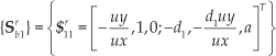
The independence between each limb constraint-screw system in Eqs. (12), (13) and (14) is evaluated. The linearly independent screws conform a nonunique basis for subspace $S^r$ , which can be selected as:

$〈S^r〉=〈S_{11}^r\mathrm{,}{S}_{21}^r\mathrm{,}{S}_{31}^r〉$

(15)

This shows that platform motion is subjected to three independent constraints, one in each limb. Taking the reciprocal of $〈S^r〉$ yields platform motion-screw system $\left\{S_f\right\}$ :

$\left\{S_f\right\}=\left\{{\$}_{f1}\mathrm{,}{\$}_{f2}\mathrm{,}{\$}_{f3}\right\}$

(16)

where

$\begin{array}{l}{\$}_{f1}=[\frac{3a(ux+vy)}{2d_{1}ux-(d_2+d_3)ux+\sqrt{3}(d_2-d_3)vx}\mathrm{,} \mathrm{0,} 1; (aux(\sqrt{3}\left(d_2-d_3\right)u{x}^2+ux(-2d_{1}uy+\hfill \\ \left(d_2+d_3\right)uy+\sqrt{3}\left(d_2-d_3\right)vy)+vx\left(d_3\left(\sqrt{3}uy+3\sqrt{3}vx-3vy\right)+6d_{1}vy-d_2\left(\sqrt{3}uy+3\left(\sqrt{3}vx+vy\right)\right)\right)))/\hfill \\ \left(2\left(2d_{1}ux-(d_2+d_3)ux+\sqrt{3}\left(d_2-d_3\right)vx\right)\left(-uyvx+uxvy\right)\right)\mathrm{,} (a\left(2\sqrt{3}{d}_{1}ux\left(-uy(uy+vx\right)+vy\left(ux+3vy\right)\right)\hfill \\ +d_3\left(ux\left(uy-2vx\right)\left(\sqrt{3}uy-3vy\right)+3uyvx\left(uy+vx-\sqrt{3}vy\right)+u{x}^2\left(-3uy+2\sqrt{3}vy\right)\right)\hfill \\ +d_2\left(ux\left(uy-2vx\right)\left(\sqrt{3}uy+3vy\right)-3uyvx\left(uy+vx+\sqrt{3}vy\right)+u{x}^2\left(3uy+2\sqrt{3}vy\right)\right)))/(2\sqrt{3}(2d_{1}ux\hfill \\ {-\left(d_2+d_3\right)ux+\sqrt{3}\left(d_2-d_3\right)vx)\left(-uyvx+uxvy\right)))\mathrm{,} 0]}^T\hfill \\ {\$}_{f2}=[\frac{-2d_{1}uy+(d_2+d_3)uy+\sqrt{3}(-d_2+d_3)vy}{2d_{1}ux-(d_2+d_3)ux+\sqrt{3}(d_2-d_3)vx}\mathrm{,} \mathrm{1,} 0; \frac{2d_2{d}_{3}ux-d_1(d_2+d_3)ux+\sqrt{3}{d}_1(-d_2+d_3)vx}{2d_{1}ux-(d_2+d_3)ux+\sqrt{3}(d_2-d_3)vx}\mathrm{,} \hfill \\ {\frac{2d_2{d}_{3}uy-d_1(d_2+d_3)uy+\sqrt{3}{d}_1(-d_2+d_3)vy}{2d_{1}ux-(d_2+d_3)ux+\sqrt{3}(d_2-d_3)vx}\mathrm{,} 0]}^T\hfill \\ {\$}_{f3}={\left[\mathrm{0,} \mathrm{0,} 0; \mathrm{0,} \mathrm{0,} 1\right]}^T\hfill \end{array}$

The obtained platform motion-screw system is described relative to the $G(X\mathrm{,}Y\mathrm{,}Z)$ frame. Note that Eq. (16) demonstrates that the 3-CRC PM belongs to the 2R1T family, since the moving platform has three DOF, i.e. $F=3$ (where F is the number of DOF), namely two rotations about the skew axes given by ${\$}_{f1}$ and ${\$}_{f2}$ , and a translation along the Z axis as shown by ${\$}_{f3}$ . Furthermore, it is possible to observe from Eq. (16) that the ${\$}_{f1}$ has a rotation in a skew axis that lies on the $XZ$ plane and parasitic displacement on the $XY$ plane. In addition, ${\$}_{f2}$ rotates about a skew axis on the $XY$ plane and parasitic movement on the $XY$ plane. As a general definition, a parasitic motion is a dependent movement produced by the degrees-of-freedom of the platform. These motions are an undesired behaviour of PMs, which are intrinsic in lower mobility PMs and in some applications these can be detrimental [21]. This moving platform experiences two parasitic motions on the $XY$ plane, which are dependent on the two rotational DOF of the platform and indicate that the 3-CRC PM does not have centralized motion[14], i.e. the centroid of the platform is not coincident with the Z axis for all configurations of the mechanism.

4. Position Analysis of the 3-CRC

This paper includes the inverse and forward position analysis of the PM. The inverse position analysis consists of determining the magnitude of the actuators’ strokes in order to reach the desired pose of the end-effector.

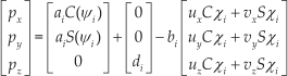
The loop closure equation for limb i relative to frame $G(X\mathrm{,}Y\mathrm{,}Z)$ and is defined as:

$p{+}^G{b}_i=a_i+d_i$

(17)

The loop closure equation represents the position of the centroid C relative to the global reference frame $G(X\mathrm{,}Y\mathrm{,}Z)$ . Substituting Eqs. (6) and (8) into Eq. (17) results in the following loop closure equation:

$\left[\begin{array}{c}{p}_x\\ p_y\\ p_z\end{array}\right]=\left[\begin{array}{c}{a}_{i}C({\psi }_i)\\ a_{i}S({\psi }_i)\\ 0\end{array}\right]+\left[\begin{array}{c}0\\ 0\\ d_i\end{array}\right]-b_i\left[\begin{array}{c}{u}_{x}C{\chi }_i+v_{x}S{\chi }_i\\ u_{y}C{\chi }_i+v_{y}S{\chi }_i\\ u_{z}C{\chi }_i+v_{z}S{\chi }_i\end{array}\right]$

(18)

According to the mobility analysis performed in the previous section, the positioning of the platform is given by one independent translational DOF along the Z -axis and two parasitic translations along the X and Y axes. Furthermore, the orientation is defined by two rotations about skew axes on the $XY$ and $XZ$ planes. The position of the centroid C is represented by p_z and the orientation of the platform by the α and β angles. A system of nine equations is defined when Eq. (18) is written for each limb and is solved for the unknown variables d_i and b_i for each limb, as well as for p_x, p_y and γ. The commercial software Mathematica 10 is used to solve the Eq. (18) by considering α, β, p_z, a, ψ_i and χ_i as input parameters.

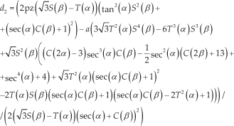
Solving the system, the actuator strokes are defined by d₁, d₂ and d₃ in Eq.(4) as follows:

$\begin{array}{l}\begin{array}{l}{d}_1=(-6aS\left(\alpha \right)T\left(\alpha \right)T^3\left(\beta \right)+aT\left(\beta \right)(-C\left(2\alpha \right)(2\sec \left(\alpha \right)+\\ +3\sec \left(\beta \right))-\sec \left(\beta \right)\left(6C\left(\alpha \right)\sec \left(\beta \right)+7\right))+2aS\left(\beta \right)\end{array}\hfill \\ \begin{array}{l}+2S^2\left(\alpha \right)T^2\left(\beta \right)\left(2\text{pz}-3aS\left(\beta \right)\right)+4\text{pz}{\left(C\left(\alpha \right)\sec \left(\beta \right)+1\right)}^2)/\\ /\left(4{\left(C\left(\alpha \right)+\sec \left(\beta \right)\right)}^2\right)\end{array}\hfill \end{array}$

(19)

$\begin{array}{l}\begin{array}{l}{d}_2=(2\text{pz}\left(\sqrt{3}S\left(\beta \right)-T\left(\alpha \right)\right)({{\displaystyle \tan }}^2\left(\alpha \right)S^2\left(\beta \right)+\\ +{\left(\sec \left(\alpha \right)C\left(\beta \right)+1\right)}^2)-a(3\sqrt{3}{T}^2\left(\alpha \right)S^4\left(\beta \right)-6T^3\left(\alpha \right)S^3\left(\beta \right)\end{array}\hfill \\ \begin{array}{l}+\sqrt{3}{S}^2\left(\beta \right)(\left(C\left(2\alpha \right)-3\right){{\displaystyle \sec }}^3\left(\alpha \right)C\left(\beta \right)-\frac{1}{2}{{\displaystyle \sec }}^2\left(\alpha \right)\left(C\left(2\beta \right)+13\right)+\\ +{{\displaystyle \sec }}^4\left(\alpha \right)+4)+\sqrt{3}{T}^2\left(\alpha \right){\left(\sec \left(\alpha \right)C\left(\beta \right)+1\right)}^2\end{array}\hfill \\ \begin{array}{l}-2T\left(\alpha \right)S\left(\beta \right)\left(\sec \left(\alpha \right)C\left(\beta \right)+1\right)\left(\sec \left(\alpha \right)C\left(\beta \right)-2T^2\left(\alpha \right)+1\right)))/\\ /\left(2\left(\sqrt{3}S\left(\beta \right)-T\left(\alpha \right)\right){\left(\sec \left(\alpha \right)+C\left(\beta \right)\right)}^2\right)\end{array}\hfill \end{array}$

(20)

$\begin{array}{l}\begin{array}{l}{d}_3=\left(2\text{pz}(T\left(\alpha \right)+\sqrt{3}S\left(\beta \right)\right)(T^2\left(\alpha \right)S^2\left(\beta \right)+\\ +\left(\sec \left(\alpha \right)C\left(\beta \right)+{1)}^2\right)-a(3\sqrt{3}{T}^2\left(\alpha \right)S^4\left(\beta \right)+6T^3\left(\alpha \right)S^3\left(\beta \right)\end{array}\hfill \\ \begin{array}{l}+\sqrt{3}{S}^2\left(\beta \right)(\left(C\left(2\alpha \right)-3\right){{\displaystyle \sec }}^3\left(\alpha \right)C\left(\beta \right)-\frac{1}{2}{{\displaystyle \sec }}^2\left(\alpha \right)\left(C\left(2\beta \right)+13\right)+\\ +{{\displaystyle \sec }}^4\left(\alpha \right)+4)+\sqrt{3}{T}^2\left(\alpha \right){\left(\sec \left(\alpha \right)C\left(\beta \right)+1\right)}^2\end{array}\hfill \\ \begin{array}{l}+2T\left(\alpha \right)S\left(\beta \right)(\sec \left(\alpha \right)C\left(\beta \right)+1)\left(\sec \left(\alpha \right)C\left(\beta \right)-2T^2\left(\alpha \right)+1\right)))/\\ /\left(2\left(T\left(\alpha \right)+\sqrt{3}S\left(\beta \right)\right){\left(\sec \left(\alpha \right)+C\left(\beta \right)\right)}^2\right)\end{array}\hfill \end{array}$

(21)

The strokes for joints $j_{i5}$ result in:

$\begin{array}{l}\begin{array}{l}{b}_1=\left(a(3S\left(\alpha \right)T\left(\alpha \right)S\left(\beta \right)T\left(\beta \right)-\sec \left(\alpha \right)C\left(\beta \right)+3C\left(\alpha \right)\sec \left(\beta \right)+2\right)/\\ /\left(2\sqrt{{\left(C\left(\alpha \right)C\left(\beta \right)+1\right)}^2}\right)\end{array}\hfill \end{array}$

(22)

$\begin{array}{l}\begin{array}{l}{b}_2=(a(108T^2\left(\alpha \right)S^5\left(\beta \right)-4\sqrt{3}{T}^3\left(\alpha \right)\sec \left(\alpha \right)\\ \left(C\left(\alpha \right)+C\left(\beta \right)\right)-3\sqrt{3}T\left(\alpha \right){{\displaystyle \sec }}^3\left(\alpha \right)S^2\left(\beta \right)(4C\left(2\alpha \right)(\sec \left(\alpha \right)\end{array}\hfill \\ \begin{array}{l}+3C\left(\beta \right))+\left(5C\left(4\alpha \right)+3\right)\sec \left(\alpha \right))+36\sqrt{3}T\left(\alpha \right)S^4\left(\beta \right)(\sec \left(\alpha \right)(C\left(\beta \right)-\\ -3\sec \left(\alpha \right))+5)+36S^3\left(\beta \right)(\sec \left(\alpha \right)C\left(\beta \right)\end{array}\hfill \\ \begin{array}{l}-3T^2\left(\alpha \right)\left(\sec \left(\alpha \right)C\left(\beta \right)+2\right)+3T^4\left(\alpha \right)+1)+\\ +12T^2\left(\alpha \right)S\left(\beta \right)\left(3\sec \left(\alpha \right)C\left(\beta \right)+T^2\left(\alpha \right)\left(-\left(\sec \left(\alpha \right)C\left(\beta \right)+2\right)\right)+3\right)))\end{array}\hfill \\ \begin{array}{l}/4\sqrt{{\left(C\left(\alpha \right)C\left(\beta \right)+1\right)}^2}(9\sqrt{3}T\left(\alpha \right)S^4\left(\beta \right)+\left(9-27T^2\left(\alpha \right)\right)S^3\left(\beta \right)+\\ +9\sqrt{3}T\left(\alpha \right)\left(T^2\left(\alpha \right)-1\right)S^2\left(\beta \right)-\end{array}\hfill \\ -3T^2\left(\alpha \right)\left(T^2\left(\alpha \right)-3\right)S\left(\beta \right)-\sqrt{3}{T}^3\left(\alpha \right)))\hfill \end{array}$

(23)

$\begin{array}{l}\begin{array}{l}{b}_3=(aC\left(\alpha \right)(-9S\left(\alpha \right)T\left(\alpha \right)S^3\left(\beta \right)-\sqrt{3}T\left(\alpha \right)(C\left(\alpha \right)+\\ +C\left(\beta \right))+3\sqrt{3}T\left(\alpha \right)S^2\left(\beta \right)\left(S\left(\alpha \right)T\left(\alpha \right)+C\left(\beta \right)\right)\end{array}\hfill \\ \begin{array}{l}+3S\left(\beta \right)\left(C\left(2\alpha \right){{\displaystyle \sec }}^2\left(\alpha \right)C\left(\beta \right)+C\left(\alpha \right)\right)))/\\ /\left(\sqrt{{\left(C\left(\alpha \right)C\left(\beta \right)+1\right)}^2}\left(\sqrt{3}S\left(\alpha \right)C\left(\alpha \right)\left(3S^2\left(\beta \right)-1\right)+3C\left(2\alpha \right)S\left(\beta \right)\right)\right)\end{array}\hfill \end{array}$

(24)

The position of the platform in the $XY$ plane is defined by p_x and p_y, while rotation about the Z -axis is defined by the γ angle, which can be expressed as follows:

$\begin{array}{l}{p}_x=\frac{a\left(\sec \left(\alpha \right)C\left(\beta \right)-1\right){\left(\sec \left(\alpha \right)C\left(\beta \right)+1\right)}^2-a{T}^2\left(\alpha \right)S^2\left(\beta \right)\left(3\sec \left(\alpha \right)C\left(\beta \right)+1\right)}{2{\left(\sec \left(\alpha \right)+C\left(\beta \right)\right)}^2}\hfill \end{array}$

(25)

$\begin{array}{l}{p}_y=-\frac{aT\left(\alpha \right)S\left(\beta \right)\left(3S^2\left(\alpha \right)S^2\left(\beta \right)+\left(3C\left(\alpha \right)-C\left(\beta \right)\right)\left(C\left(\alpha \right)+C\left(\beta \right)\right)\right)}{2{\left(C\left(\alpha \right)C\left(\beta \right)+1\right)}^2}\hfill \end{array}$

(26)

$\begin{array}{l}\gamma =\arctan \left(-\frac{S\left(\alpha \right)S\left(\beta \right)}{C\left(\alpha \right)+C\left(\beta \right)}\right)\hfill \end{array}$

(27)

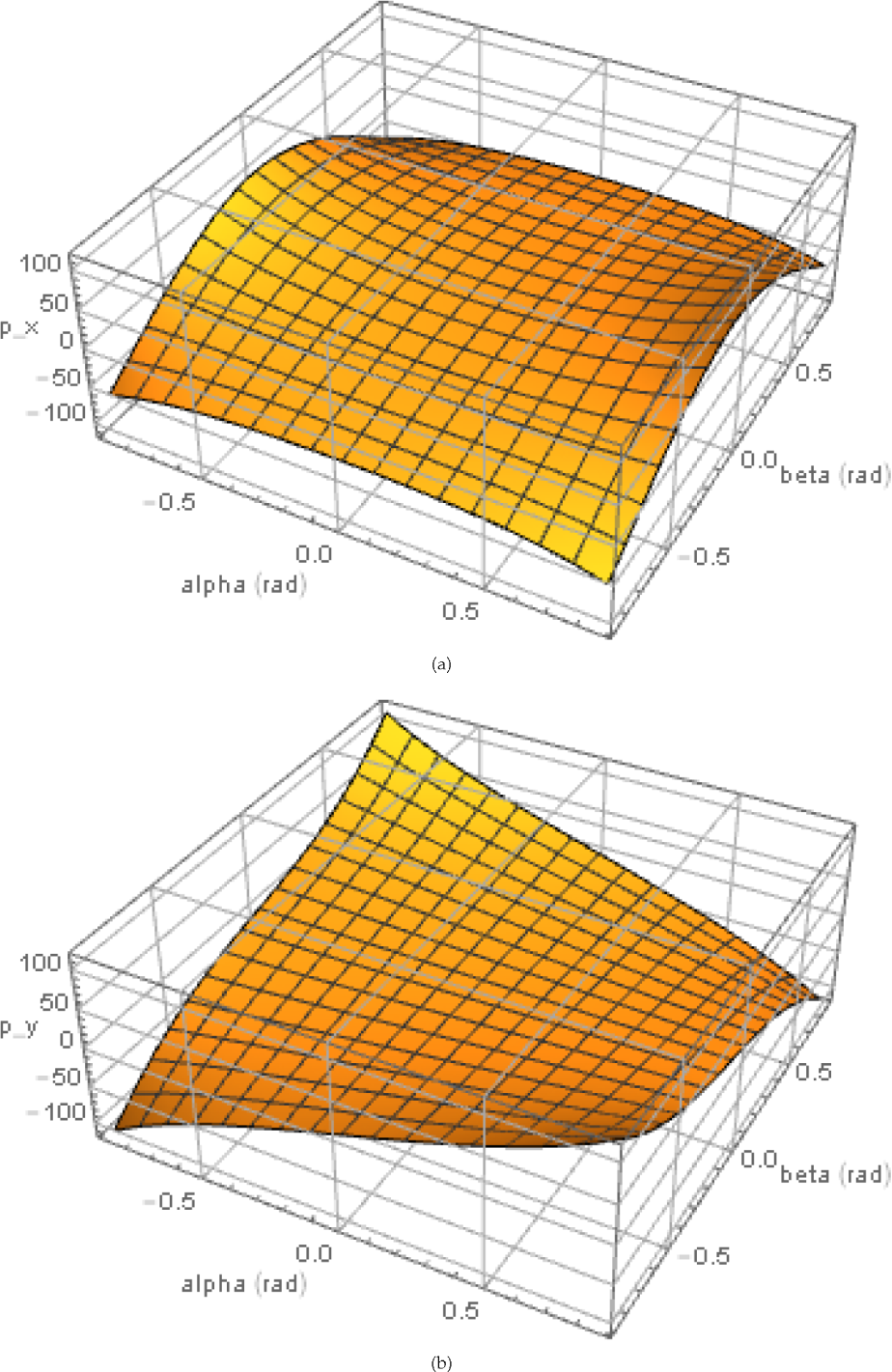
The literature shows that parasitic motions are a major drawback of the general 2R1T PM, since this issue results in complex kinematics that require real-time compensation and also increases difficulties in calibration, leading to possible damage[22]. For the 3-CRC PM, parasitic motions are fully defined for all the configurations of the mechanism by p_x, p_y and γin Eqs. (25)–(27); see Figs. 3(a) and 3(b), which illustrate the undesired motions in the X -axis and Y -axis, respectively.

Figure 3.

Parasitic Motion (a)in the X-axis, (b)in the Y-axis

The direct kinematic problem is well-known in the literature and consists of determining the pose of the moving platform when the input of the magnitude of the strokes of d₁, d₂ and d₃ is known. The pose is composed by the position vector $p$ , while the orientation is defined by the α, β and γ angles. This problem is approached by analysing the position and orientation of the platform independently.

This plane is defined by the points ${\mathrm{B}}_1$ , ${\mathrm{B}}_2$ and ${\mathrm{B}}_3$ , as shown in Fig. 4, where each point ${\mathrm{B}}_i$ is described by $r_{i3}$ , which is related to frame G and is defined as follows:

$r_{i3}=\left[\begin{array}{c}{a}_{i}C\left({\psi }_i\right)\\ a_{i}S\left({\psi }_i\right)\\ d_i\end{array}\right] for i=\mathrm{1,2,} and 3$

(28)

Figure 4.

Vectors q ₁ and q ₂ to determine the orientation of moving platform

The vectors $q_1$ and $q_2$ that lie on the platform $UV$ plane (see Fig. 4) are defined as $q_1=r_{23}-r_{13}$ and $q_2=r_{33}-r_{13}$ . Note that a normal vector to this plane can be obtained as a result of the cross product of $q_1$ and $q_2$ , namely:

$n=q_1\times q_2={\left[n_x\mathrm{,} n_y\mathrm{,} n_z\right]}^T$

(29)

where a unit vector $\widehat{n}$ can be obtained from Eq. (29) as follows:

$\widehat{n}=n/\left|n\right|={\left[{\widehat{n}}_x\mathrm{,} {\widehat{n}}_y\mathrm{,} {\widehat{n}}_z\right]}^T$

(30)

Vector $\widehat{n}$ in Eq. (30) is expressed in the platform frame H and can be transformed to the general frame G as follows:

${\left[{\widehat{n}}_x\mathrm{,} {\widehat{n}}_y\mathrm{,} {\widehat{n}}_z\right]}^T{=}^G{R}_H\cdot {\left[0 0 1\right]}^T$

(31)

where

${\widehat{n}}_x=S(\beta )$

(32)

${\widehat{n}}_y=-S(\alpha )C(\beta )$

(33)

${\widehat{n}}_z=C(\alpha )C(\beta )$

(34)

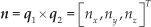
A geometric method is applied in order to obtain the α angle as proposed in [15]. Fig. 5 presents the geometrical constraints that are necessary to define the α angle, whose magnitude depends on the strokes d₂ and d₃ as observed in Eqs. (32)–(34). It can further be seen that α is defined between the Y - and V - axes.

$\alpha =\arctan \left(d_2-d_3/\left|a*S({\psi }_3)\right|+\left|a*S({\psi }_2)\right|\right)$

(35)

Figure 5.

Geometrical analysis to compute the angle α based on [15]

The β angle can be calculated from Eq.(34). Note that computation of the β angle depends on the result of the inverse cosine, where only one result is accepted, considering the geometry of the manipulator. Therefore, a sign function is applied for convenience purposes.

$\beta =\arccos \left[{\widehat{n}}_z/C(\alpha )\right]\text{Sign}\left[\left(\left(d_2+d_3\right)/2\right)-d_1\right]$

(36)

Four simulations are performed in Solidworks in order to validate the geometric approach for obtaining the closed-form solution of α in Eq. (35). Consider that in simulation (i) $d_2(t)=d_3(t)$ and $d_1(t)\ne [d_2(t)\hspace{0.17em}\&\hspace{0.17em}{d}_3(t)]$ ; (ii) $d_2(t)=d_3(t)$ and d₁ is constant; (iii) $d_2\ne d_3$ , while $d_1(t)$ ; (iv) $d_2(t)\ne d_3(t)\ne d_1(t)$ . Table 1 shows the parameters for the above-mentioned cases. Consider that d₁, d₂ and d₃ are given by a slope equation for time (t) and note that the value of α depends directly on d₁ and d₂; if d₁ and d₂ have the same value then $\alpha {=0}^{\circ }$ as in simulations 1 and 2; for any other case the angle α is different to zero as in simulations 3 and 4.

Fig. 6(a) and Fig. 6(b) show that while d₂ and d₃ remain of equal magnitude, the α angle is equal to $0^{\circ }$ , despite the variation in time of the stroke of d₂ and d₃. Furthermore, Fig. 6(c) shows that if d₂ and d₃ are fixed but with different magnitudes, then the α angle is different than zero. In addition, Fig. 6(d) indicates that if d₂ and d₃ are different and variable over time, the α angle is different than zero and variable in time according to Eq. (35).

Table 1.

Orientation simulation parameters

Parameter	Simulation 1	Simulation 2	Simulation 3	Simulation 4
time (s)	10	10	10	10
a(mm)	184.75	184.75	184.75	184.75
d1(mm)	552+(−6.7*t+136)	852	552+(17.9*t+69)	552+(−6.7*t+136)
d2 (mm)	552+(−4.5*t+69)	552+(−6.7*t+136)	552	552+(−4.5*t+69)
d3 (mm)	552+(−4.5*t+69)	552+(−6.7*t+136)	852	552+(17.9*t+69)
α (deg)	0°	0°	−43.15°	from 0° to −34.99°

The equations obtained from the solution of the inverse kinematics problem for the parasitic positions in Eqs. (25) and (26) show that these are dependent on the α and β angles; at the same time, these angles are dependent on the strokes of the passive cylindrical joints of the moving platform in Eq. (22)–(24), where all these equations are used to compute the position of the platform in the Z-axis from the closed-loop in Eq. (18):

$p_z=d_i-b_i\left[u_{z}C{\chi }_i+v_{z}S{\chi }_i\right]$

(37)

In order to clarify the analytical results that were previously obtained, a numerical exercise is performed as follows.

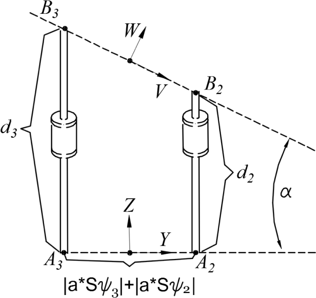
Numerical Example 1. A numerical exercise is performed in order to demonstrate the validity and consistency of the analytical results of the closed-form solutions for the inverse and direct kinematics when compared to motion simulations. This exercise is performed by means of a CAD model of the 3-CRC PM using Solidworks software and numerical computations alongside software Mathematica. The results of this exercise are shown in Table 2.

As shown in Table 2, the corresponding results for the initial and final pose to the inverse and direct kinematics are shown in the first and second column, respectively. Note that the input parameters for each analysis are expressed in bold type lettering i.e. p_z, α and β for the inverse kinematics, while d₁, d₂ and d₃ in the second column corresponds to the parameters for the direct kinematics. For this example, the computation considers that the input parameters for the direct kinematics correspond to the output results of the inverse kinematics. The third column in Table 2 presents the parameters obtained by the CAD software, where d₁, d₂ and d₃ are set in the model and the remainder of the parameters are measured and reported.

Figure 6.

α Angle Magnitudes for (a) Simulation 1, (b) Simulation 2, (c) Simulation 3 and (d) Simulation 4

Table 2.

Pose numerical Exercise 1

	Initial Pose			Final Pose
Parameters	Inverse Kinematic	Direct Kinematic	CAD model	Inverse Kinematic	Direct Kinematic	CAD model
a (mm)	184.75	184.75	184.75	184.75	184.75	184.75
d1 (mm)	687.995	688	688	621.009	621	621
d2 (mm)	621.002	621	621	575.997	576	576
d3 (mm)	621.002	621	621	799.978	800	800
b1 (mm)	192.732	192.732	192.736	171.798	171.798	171.801
b2 (mm)	184.750	184.750	184.752	200.960	200.96	200.958
b3 (mm)	184.750	184.750	184.752	249.201	249.201	249.217
px (mm)	-2.586	-2.586	-2.586	16.546	16.546	16.546
py (mm)	0.000	0.000	0.000	10.407	10.407	10.410
pz (mm)	642.708	642.708	642.708	654.378	654.384	654.378
α (deg)	0	0.00	0	-34.99	-34.99	-34.99
β (deg)	-13.59	-13.59	-13.59	11.20	11.19	11.20
γ (deg)	0.00	0.00	0.00	3.54	3.54	3.54

Note that the results presented in the third column of Table 2 are obtained from the function of displacement measure and Bryant angles in Solidworks, where the maximum discrepancy of the results compared to the simulation show an error of $0.00275\%$ , which is significantly low, despite the complexity of the closed form solution and with higher precision when compared to other 2R1T architectures, as reported in [15]. Concerning the parasitic motions that are fully determined during the simulations and numeric exercises, these are considered acceptable due to their limited magnitude. However, a remaining problem is to determine the maximal amplitude of these motions, given manufacturing tolerances and other sources of uncertainties[23].

According to the results computed in Exercise 1, the initial and final pose can be compared with the simulation obtained from the CAD software package. Figure 7 shows the pose of the moving platform, where Fig. 7(b) is the position of the centroid and Fig. 7(c) is the orientation of the moving platform. The validation and accuracy of the analytical equations obtained in this paper for the inverse and direct kinematics are demonstrated according to the data comparison between the simulation from CAD and the computed results in Exercise 1.

Figure 7.

Moving platform pose: (a) Displacement of cilinders (b) Moving platform position for the 3-CRC PM, (c) Moving platform orientation for the 3-CRC PM

5. Velocity Analysis

The velocity analysis, also known as the instantaneous kinematics analysis, relates the input and output velocities of any mechanism through the use of mathematical expressions, i.e. the Jacobian matrix. The Jacobian matrix can be determined by applying the theory of reciprocal screws and by using a method proposed by Joshi and Tsai in [18]; this approach is particularly useful for studying limited-DOF parallel manipulators. It is important to observe that the methodology presented by Joshi and Tsai in [18] leads to the determination of the inverse instantaneous kinematics, including an analytical proof for two PMs, where no demonstration of the direct instantaneous kinematics is presented.

A summary of the method presented in [18] for obtaining the Jacobian matrix, which relates the velocities of the actuators with the velocities of the moving platform, is presented as follows:

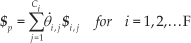
• Calculate the instantaneous twist of the moving platform $_p, which can be expressed as a linear combination of C_i instantaneous twists:

${\$}_p={\displaystyle \sum _{j=1}^{C_i}}{\dot{\theta }}_{i\mathrm{,}j}{\$}_{i\mathrm{,}j} for i=\mathrm{1,2,}\dots \mathrm{F}$

(38)

where C_i is the DOF associated with all the joints of the i th limb, F is the number of limbs, ${\dot{\theta }}_{i\mathrm{,}j}$ denotes the magnitude of the active joint velocity and ${\$}_{i\mathrm{,}j}$ represents a unit screw that is associated with the j th joint of the i th limb. The twist of the moving platform is defined as ${\$}_p={\left[{\omega }^T\hspace{0.17em}\hspace{0.17em}{\nu }_p^T\right]}^T$ , where $\omega$ is the angular velocity of the moving platform and ${\nu }_p$ is the linear velocity of a point in the moving platform that is instantaneously coincident with the origin of the reference frame in which the screws are expressed [18].

• Perform the calculation of the Jacobian of constraints, which is composed by those screws that are reciprocal to all the joint screws of the i th limb to form a $(6-C_i)$ reciprocal screw system. The ${\$}_{r\mathrm{,}i\mathrm{,}{k}_i}$ denote the k th reciprocal unit screw of the i th limb. Taking the orthogonal product of both sides of Eq. (38) with each of the $(6-C_i)$ reciprocal unit screw yields: [18]:

${\$}_{r\mathrm{,}i\mathrm{,}{k}_i}^T{\$}_p=0 for k_i=\mathrm{1,2,}\dots 6-C_i$

(39)

Equation (39) written once for each limb produces ${\displaystyle {\sum }_{i=1}^F}(6-C_i)$ equations, which can be written in matrix form as $Jc$ in Eq. (39) resulting in:

$Jc{\$}_p=0$

(40)

where

$J_c=\left[\begin{array}{c}{\$}_{r\mathrm{,1,}{k}_1}^T\\ {\$}_{r\mathrm{,2,}{k}_2}^T\\ ⋮\\ {\$}_{r\mathrm{,}F\mathrm{,}{k}_F}^T\end{array}\right]$

• Compute the Jacobian of actuation by locking the actuated joint of each limb, followed by obtaining the reciprocal screws for the remainder joint screws. Note that the dimension of the reciprocal screw system is increased by one, hence the new reciprocal unit screw is denoted as ${\$}_{r\mathrm{,}i\mathrm{,}{k}_i+1}$ , which represents a wrench of actuation. Let the g_i th joint in the i th limb be actuated and taking the orthogonal product of both sides of Eq. (38) with ${\$}_{r\mathrm{,}i\mathrm{,}{k}_i+1}$ , the following is obtained [18]:

${\$}_{r\mathrm{,}i\mathrm{,}{k}_i+1}^T{\$}_p={\dot{\theta }}_{g_i\mathrm{,}i}{\$}_{r\mathrm{,}i\mathrm{,}{k}_i+1}^T{\$}_{g_i\mathrm{,}i}$

(41)

Note that the new reciprocal screw is reciprocal to all the joint screws, except for the actuated joint screw. Writing Eq. (41) for each limb produces F equations that can be written in matrix form as:

$J_x{\$}_p=J_q\dot{q}$

(42)

where

$\begin{array}{c}{J}_x=\left[\begin{array}{c}{\$}_{r\mathrm{,1,}{k}_1+1}^T\\ {\$}_{r\mathrm{,2,}{k}_2+1}^T\\ ⋮\\ {\$}_{r\mathrm{,}\mathrm{F}\mathrm{,}{k}_{\mathrm{F}}+1}^T\end{array}\right]\\ J_q=\left[\begin{array}{cccc}{\$}_{r\mathrm{,1,}{k}_1+1}^T{\$}_{g_1\mathrm{,1}}& 0& \dots & 0\\ 0& {\$}_{r\mathrm{,2,}{k}_2+1}^T{\$}_{g_2\mathrm{,2}}& \dots & 0\\ ⋮& ⋮& ⋮& ⋮\\ 0& 0& \dots & {\$}_{r\mathrm{,}\mathrm{F}\mathrm{,}{k}_{\mathrm{F}}+1}^T{\$}_{g_{\mathrm{F}}\mathrm{,}\mathrm{F}}\end{array}\right]\\ \dot{q}=\left[{\dot{\theta }}_{g_1\mathrm{,1}}\mathrm{,} {\dot{\theta }}_{g_2\mathrm{,2}}\mathrm{,} \dots \mathrm{,} {\dot{\theta }}_{g_{\mathrm{F}}\mathrm{,}\mathrm{F}}\right]\end{array}$

Where $J_x$ is the matrix composed by the ${\$}_{r\mathrm{,}i\mathrm{,}{k}_i+1}^T$ for each limb; $J_q$ is a diagonal matrix composed by the orthogonal multiplication of ${\$}_{r\mathrm{,}i\mathrm{,}{k}_i+1}$ and ${\$}_{g_i\mathrm{,}i}$ , and vector $\dot{q}$ is composed of ${\dot{\theta }}_{g_i\mathrm{,}j}$ , which denotes the speed magnitude of the actuated joint. Note that $J_x$ is a $\mathrm{F}\times 6$ matrix and $J_q$ is a $\mathrm{F}\times \mathrm{F}$ diagonal matrix. Multiplying both sides of Eq. (42) by $J_q{}^{-1}$ yields [18]:

$\dot{q}=J_a{\$}_p$

(43)

where

$J_a=J_q{}^{-1}{J}_x=\left[\begin{array}{c}{\$}_{r\mathrm{,1,}{k}_1+1}^T/({\$}_{r\mathrm{,1,}{k}_1+1}^T{\$}_{g_1\mathrm{,1}})\\ {\$}_{r\mathrm{,2,}{k}_2+1}^T/({\$}_{r\mathrm{,2,}{k}_2+1}^T{\$}_{g_2\mathrm{,2}})\\ ⋮\\ {\$}_{r\mathrm{,}\mathrm{F}\mathrm{,}{k}_{\mathrm{F}}+1}^T/({\$}_{r\mathrm{,}\mathrm{F}\mathrm{,}{k}_{\mathrm{F}}+1}^T{\$}_{g_{\mathrm{F}}\mathrm{,}\mathrm{F}})\end{array}\right]$

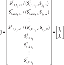
• Substitute Eq. (43) and (40) for obtaining the overall Jacobian matrix ( $J$ ) [18] as follows:

${\dot{q}}_0=J{\$}_p$

(44)

where

$J=\left[\begin{array}{c}{\$}_{r\mathrm{,1,}{k}_1+1}^T/({\$}_{r\mathrm{,1,}{k}_1+1}^T{\$}_{g_1\mathrm{,1}})\\ {\$}_{r\mathrm{,2,}{k}_2+1}^T/({\$}_{r\mathrm{,2,}{k}_2+1}^T{\$}_{g_2\mathrm{,2}})\\ ⋮\\ {\$}_{r\mathrm{,}\mathrm{F}\mathrm{,}{k}_{\mathrm{F}}+1}^T/({\$}_{r\mathrm{,}\mathrm{F}\mathrm{,}{k}_{\mathrm{F}}+1}^T{\$}_{g_{\mathrm{F}}\mathrm{,}\mathrm{F}})\\ {\$}_{r\mathrm{,1,}{k}_1}^T\\ {\$}_{r\mathrm{,2,}{k}_2}^T\\ ⋮\\ {\$}_{r\mathrm{,}\mathrm{F}\mathrm{,}{k}_{\mathrm{F}}}^T\end{array}\right]=\left[\begin{array}{c}{J}_a\\ J_c\end{array}\right]$

(45)

${\dot{q}}_0=\left[\begin{array}{c}{\dot{q}}_{\mathrm{F}\times 1}\\ 0_{(6-\mathrm{F})\times 1}\end{array}\right]$

(46)

The overall Jacobian matrix $J$ in Eq. (45) fully characterizes the instantaneous motion of the moving platform; $J$ is composed of the Jacobian of actuation in Eq. (43) and the Jacobian of constraint in Eq. (40), which generates a square matrix of dimension $6\times 6$ , where the $J_a$ matrix transforms the linear and angular velocities of the moving platform to the input joint, and the $J_c$ matrix constraints and the instantaneous motion of the moving platform to F DOF. In addition, ${\dot{q}}_0$ is a $6\times 1$ vector that is composed of vectors ${\dot{q}}_{F\times 1}$ and $0_{(6-\mathrm{F})\times 1}$ , which enables the correct operation of multiplying $J$ and ${\$}_p$ of Eq. (44). Note that in the method proposed in [18], where the vector $0_{(6-\mathrm{F})\times 1}$ have only zeros, therefore they considered quite irrelevant the possible results of multiply the matrix J_c by vector $_p.

Following the above-noted steps, determination of the inverse instantaneous kinematics for the 3-CRC is presented. For this PM, the instantaneous twist of Eq. (38) corresponds to a linear combination of five instantaneous twists:

${\$}_p={\dot{d}}_{i1}{\$}_{i1}+{\dot{\theta }}_{i2}{\$}_{i2}+{\dot{\theta }}_{i3}{\$}_{i3}+{\dot{\theta }}_{i4}{\$}_{i4}+{\dot{b}}_{i5}{\$}_{i5}$

(47)

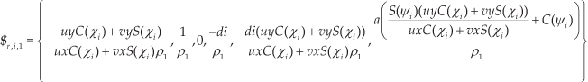
This PM possesses only one reciprocal screw for each limb, which is the general reciprocal screw ${\$}_{r\mathrm{,}i\mathrm{,1}}$ and which can be determined from the motion screw system in Eq. (11):

${\$}_{r\mathrm{,}i\mathrm{,1}}=\left\{-\frac{uyC({\chi }_i)+vyS({\chi }_i)}{uxC({\chi }_i)+vxS({\chi }_i)}\mathrm{,1,0,}-di\mathrm{,}-\frac{di(uyC({\chi }_i)+vyS({\chi }_i))}{uxC({\chi }_i)+vxS({\chi }_i)}\mathrm{,}a\left(\frac{S({\psi }_i)(uyC({\chi }_i)+vyS({\chi }_i))}{uxC({\chi }_i)+vxS({\chi }_i)}+C({\psi }_i)\right)\right\}$

(48)

Normalizing ${\$}_{r\mathrm{,}i\mathrm{,1}}$ in Eq. (48) results in the following unit reciprocal screw ${\$}_{r\mathrm{,}i\mathrm{,1}}$ :

${\$}_{r\mathrm{,}i\mathrm{,1}}=\left\{-\frac{uyC({\chi }_i)+vyS({\chi }_i)}{uxC({\chi }_i)+vxS({\chi }_i){\rho }_1}\mathrm{,}\frac{1}{{\rho }_1}\mathrm{,0,}\frac{-di}{{\rho }_1}\mathrm{,}-\frac{di(uyC({\chi }_i)+vyS({\chi }_i))}{uxC({\chi }_i)+vxS({\chi }_i){\rho }_1}\mathrm{,}\frac{a\left(\frac{S({\psi }_i)(uyC({\chi }_i)+vyS({\chi }_i))}{uxC({\chi }_i)+vxS({\chi }_i)}+C({\psi }_i)\right)}{{\rho }_1}\right\}$

(49)

where

${\rho }_1=\sqrt{1+\frac{{\left(uyC({\chi }_i)+vyS({\chi }_i)\right)}^2}{{\left(uxC({\chi }_i)+vxS({\chi }_i)\right)}^2}}$

The Jacobian of constraint $Jc$ is obtained by applying the orthogonal product of the reciprocal unit screw for each limb according to Eq. (39) and by rearranging these results in matrix form is obtained:

$J_c=\left[\begin{array}{cccccc}\frac{-d1}{{\rho }_1}& -\frac{d1(uyC({\chi }_1)+vyS({\chi }_1))}{uxC({\chi }_1)+vxS({\chi }_1){\rho }_1}& JcA& -\frac{uyC({\chi }_1)+vyS({\chi }_1)}{uxC({\chi }_1)+vxS({\chi }_1){\rho }_1}& \frac{1}{{\rho }_1}& 0\\ \frac{-d2}{{\rho }_1}& -\frac{d2(uyC({\chi }_2)+vyS({\chi }_2))}{uxC({\chi }_2)+vxS({\chi }_2){\rho }_1}& JcB& -\frac{uyC({\chi }_2)+vyS({\chi }_2)}{uxC({\chi }_2)+vxS({\chi }_2){\rho }_1}& \frac{1}{{\rho }_1}& 0\\ \frac{-d3}{{\rho }_1}& -\frac{d3(uyC({\chi }_3)+vyS({\chi }_3))}{uxC({\chi }_3)+vxS({\chi }_3){\rho }_1}& JcC& -\frac{uyC({\chi }_3)+vyS({\chi }_3)}{uxC({\chi }_3)+vxS({\chi }_3){\rho }_1}& \frac{1}{{\rho }_1}& 0\end{array}\right]$

(50)

where

$JcA=\frac{a\left(C({\psi }_1)+\frac{(uyC({\chi }_1)+vyS({\chi }_1))S({\psi }_1)}{uxC({\chi }_1)+vxS({\chi }_1)}\right)}{{\rho }_1}$

$JcB=\frac{a\left(C({\psi }_2)+\frac{(uyC({\chi }_2)+vyS({\chi }_2))S({\psi }_2)}{uxC({\chi }_2)+vxS({\chi }_2)}\right)}{{\rho }_1}$

$JcC=\frac{a\left(C({\psi }_3)+\frac{(uyC({\chi }_3)+vyS({\chi }_3))S({\psi }_3)}{uxC({\chi }_3)+vxS({\chi }_3)}\right)}{{\rho }_1}$

Note that each row of the $J_c$ in Eq. (50) represents a wrench imposed by the joints of a limb that properly constrains the moving platform in order to display F -DOF, where the rank of $J_c$ is equal to $6-\mathrm{F}$ [18].

The Jacobian of actuation $J_a$ in Eq. (43) can be obtained after locking the actuated joint in each limb, which in this case is the $j_{i1}$ prismatic joint, which is the first P joint of each limb. Recall that this results in the generation of an additional reciprocal screw for each limb, which is arranged in the following matrix:

$J_a=\left[\begin{array}{cccccc}aS({\psi }_1)& -aC({\psi }_1)-\frac{d1(uzC({\chi }_1)+vzS({\chi }_1))}{uxC({\chi }_1)+vxS({\chi }_1)}& \frac{a(uzC({\chi }_1)+vzS({\chi }_1))S({\psi }_1)}{uxC({\chi }_1)+vxS({\chi }_1)}& -\frac{uzC({\chi }_1)+vzS({\chi }_1)}{uxC({\chi }_1)+vxS({\chi }_1)}& 0& 1\\ aS({\psi }_2)& -aC({\psi }_2)-\frac{d2(uzC({\chi }_2)+vzS({\chi }_2))}{uxC({\chi }_2)+vxS({\chi }_2)}& \frac{a(uzC({\chi }_2)+vzS({\chi }_2))S({\psi }_2)}{uxC({\chi }_2)+vxS({\chi }_2)}& -\frac{uzC({\chi }_2)+vzS({\chi }_2)}{uxC({\chi }_2)+vxS({\chi }_2)}& 0& 1\\ aS({\psi }_3)& -aC({\psi }_3)-\frac{d3(uzC({\chi }_3)+vzS({\chi }_3))}{uxC({\chi }_3)+vxS({\chi }_3)}& \frac{a(uzC({\chi }_3)+vzS({\chi }_3))S({\psi }_3)}{uxC({\chi }_3)+vxS({\chi }_3)}& -\frac{uzC({\chi }_3)+vzS({\chi }_3)}{uxC({\chi }_3)+vxS({\chi }_3)}& 0& 1\end{array}\right]$

(51)

The overall Jacobian matrix of Eq. (45) results from replacing the $J_a$ matrix of Eq. (51) and the $J_c$ matrix of Eq. (50) in order to solve Eq. (44), which is the inverse instantaneous kinematics.

It is well-established in the literature that it is possible to obtain the direct instantaneous kinematics from Eq. (44) by pre-multiplying the $J^{-1}$ matrix in both sides, resulting in:

${\$}_p=J^{-1}{\dot{q}}_0$

(52)

However, it is noted that the platform velocities obtained from Eq. (52) for lower mobility PMs result in a discrepancy of values when compared to the velocities observed in the simulation. This is due to the default use of vector ${\dot{0}}_{(6-\mathrm{F})\times 1}$ in Eq. (46).

In order to correctly perform the direct instantaneous kinematics, this paper proposes the use of vector ${\dot{q}}_h$ , which is a $(6-\mathrm{F})\times 1$ and which can be expressed as follows:

${\dot{q}}_h=\left[\begin{array}{c}{\dot{q}}_{\mathrm{F}\times 1}\\ m_h{}_{(6-\mathrm{F})\times 1}\end{array}\right]$

(53)

Where vector ${\dot{q}}_h$ is an arrangement of vectors $\dot{q}$ in Eq. (43) and $m_h$ , which represents the velocity constraints for the instantaneous motion of the moving platform given, which in turn is the result of the multiplication of matrix $J_c$ by instantaneous twist ${\$}_p$ of Eq. (44). Vector $m_h$ is important for the computation of the velocities of the moving platform in the direct instantaneous kinematics, as is demonstrated in Numerical Example 2. This vector had not previously been considered in the literature. Note that vector ${\dot{q}}_h$ includes actuator velocities and velocity constraints.

For the correct calculation of the direct instantaneous kinematics it is necessary to compute the inverse instantaneous kinematics in order to receive the values of vector $m_h$ . Hence, Eq. (44) is modified in order to compute the complete inverse instantaneous kinematics, which includes the values of vector $m_h$ for instantaneous velocity as follows:

${\dot{q}}_h=J{\$}_p$

(54)

Therefore, the direct instantaneous kinematics are computed with the inverse of the overall Jacobian in Eq. (45), which is a square matrix. The $J^{-1}$ is pre-multiplied in both sides of Eq. (54) resulting in:

${\$}_p=J^{-1}{\dot{q}}_h$

(55)

where ${\dot{q}}_h$ is expressed in Eq. (53). This vector allows for the correct calculation of the direct instantaneous kinematics.

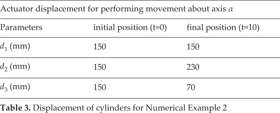
Numerical Example 2. A numerical exercise is performed in order to validate the consistency of the analytical results of the instantaneous kinematic analysis, where the most important elements are the overall Jacobian $J$ and the vector ${\dot{q}}_h$ . A simulation of the 3-CRC PM is performed in Solidworks in order to obtain the linear and angular displacement, as well as the linear and angular velocities of the moving platform. The data provided by the simulation is further compared with the results obtained from the calculation of the inverse and direct instantaneous kinematics determined in Eqs. (54) and (55).

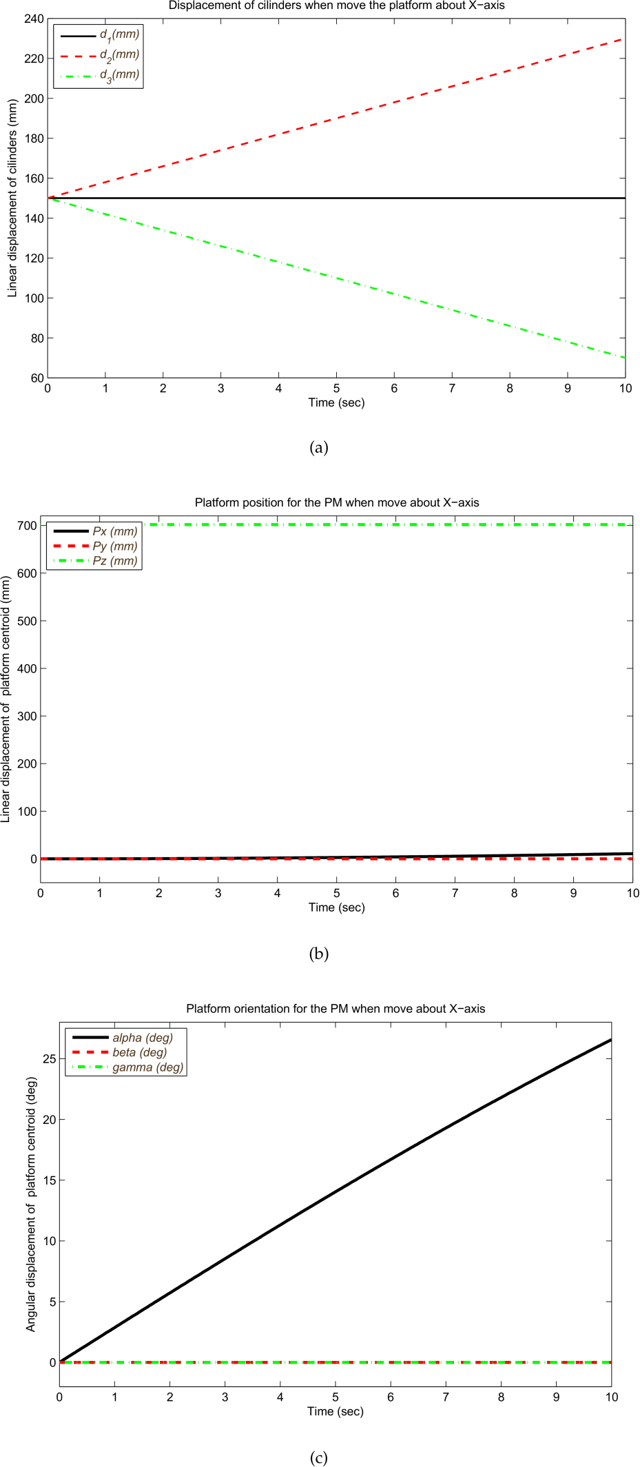
Table 3 includes the motion simulation for the α axis, which is performed in Solidworks and considers a running time of 10 seconds. Initial and final positions for each prismatic actuator is shown in Table 3:

Table 3.

Displacement of cylinders for Numerical Example 2

Actuator displacement for performing movement about axisα
Parameters	initial position (t=0)	final position (t=10)
d1 (mm)	150	150
d2 (mm)	150	230
d3 (mm)	150	70

Table 4.

Instantaneous kinematics of Initial Pose Numerical Exercise 2

Instantaneous velocity in the initial pose of the platform moving about the axisα
Parameters	Inverse instantaneous kinematics with q̇h vector	Direct instantaneous kinematics with q̇h vector	CAD simulation	Direct instantaneous kinematics with q̇0 vector
ḋ1 (mm/sec)	0	0	0	0
ḋ2 (mm/sec)	7.9996	8	8	8
ḋ3 (mm/sec)	-7.9996	-8	-8	-8
mh 1 (mm/sec)	-7.4997	-7.4997	—	0 (by default)
mh 2 (mm/sec)	-3.7498	-3.7498	—	0 (by default)
mh 3 (mm/sec)	-3.7498	-3.7498	—	0 (by default)
ωα (deg/sec)	2.8647	2.8648	2.8647	2.8648
ωβ (deg/sec)	0	0	0	0
ωγ (deg/sec)	0	0	0	0
νx (mm/sec)	0	0	0	0
νy (mm/sec)	0	0.0004	0	7.5
νz (mm/sec)	0	0	0	0

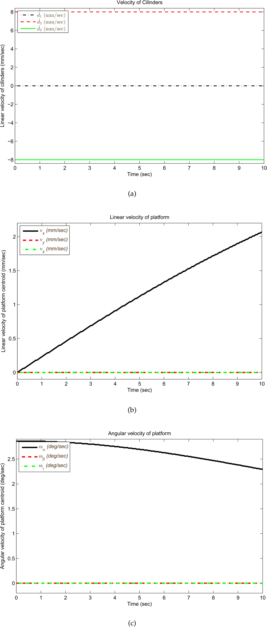
The displacement of the cylinders according to Table 3 produce linear and angular displacement of the moving platform as shown in Fig. 8. Furthermore, Fig. 9 shows the plots for the linear speed of the cylinders and the linear and angular velocities of the platform.

Figure 8.

Moving platform pose performing a rotation about axe α for the 3-CRC PM: (a) Displacement of each actuator in order to perform a rotation about α (b) Platform position according to the rotation about axis α, (c) Platform orientation according to the rotation about axis α

Note that in Tables 4 and 5, the input parameters for each analytical calculation are expressed in bold type lettering. The fourth column shows the data obtained from the simulation in Solidworks for the corresponding parameters.

Table 4 displays the analytical results of the instantaneous kinematics analysis for the initial pose of the moving platform. The inverse instantaneous kinematics is presented in the second column and is obtained by substituting the values showed in Figs. 8(a), 8(b), 8(c), 9(c) and 9(b) at the initial pose ( $t=0$ ) into Eq. (54); these analytical results are shown in standard type lettering, which corresponds to the parameters of vector ${\dot{q}}_h$ in Eq. (53). The third column shows the analytical results of the direct instantaneous kinematics by implementing Eq. (55), while the fifth column includes the results of applying (52), which does not consider the inclusion of vector ${\dot{q}}_h$ .

Figure 9.

Speed of the 3-CRC PM performing a pose: (a) Speed of each actuator in order to perform a rotation about α (b) Linear speed of the moving platform, (c) Angular speed of the moving platform according to the rotation about axis α

Table 5.

Instantaneous kinematics of Final Pose Numerical Exercise 2

Instantaneous velocity in the final pose of the platform moving about axis α
Parameters	Inverse instantaneous kinematics with q̇ h vector	Direct instantaneous kinematics with q̇ h vector	CAD simulation	Direct instantaneous kinematics with q̇ 0 vector
ḋ1(mm/sec)	0	0	0	0
ḋ2(mm/sec)	7.9997	8	8	8
ḋ3 (mm/sec)	-7.9997	-8	-8	-8
mh 1 (mm/sec)	-5.9999	-5.9999	—	0 (by default)
mh 2 (mm/sec)	-3.2539	-3.2539	—	0 (by default)
mh 3 (mm/sec)	-3.2538	-3.2538	—	0 (by default)
ωα (deg/sec)	2.2918	2.2918	2.2918	2.2918
ωβ (deg/sec)	0	0	0	0
ωγ (deg/sec)	0	0	0	0
νx (mm/sec)	2.0655	2.0655	2.0655	2.0656
νy (mm/sec)	0	0.0001	0	6
νz (mm/sec)	0	0	0	0

Furthermore, Table 5 shows the analytical results of the instantaneous kinematics analysis for the final pose of the moving platform. The inverse instantaneous kinematics is presented in the second column and is obtained by substituting the values shown in Figs. 8(a), 8(b), 8(c),9(c) and 9(b) at the final pose ( $t=10$ ) into Eq. (54), the results of which correspond to the parameters of vector ${\dot{q}}_h$ in Eq. (53). The third column displays the analytical results of the direct instantaneous kinematics by implementing Eq. (55). Finally, the fifth column includes the analytical results of Eq. (52). Tables 4 and 5 of Exercise 2 demonstrates the relevance of introducing vector $m_h{}_{(6-\mathrm{F})\times 1}$ to the method proposed by Joshi and Tsai in [18] for the correct determination of the instantaneous kinematics through the use of screw theory. The error of the analytical results using vector $m_h$ (column 3) as it relates to the CAD simulation (column 4) is $0.0143\%$ and for column 5 as it concerns column 4, the result is $261.808\%$ , shown in Table 4. Furthermore, for Table 5, the error between columns 3 and 4 is $0.004\%$ , and between columns 4 and 5 is $290.48\%$ , which means that it is necessary to consider the result of $m_{h1}$ , $m_{h2}$ and $m_{h3}$ , obtained from the inverse instantaneous kinematics, in order to obtain the correct speed for the platform as described by the twist ( ${\$}_p={\left[{\omega }^T\hspace{0.17em}\hspace{0.17em}{\nu }_p^T\right]}^T$ ).

6. Conclusion

This paper presented various kinematics analyses of a novel architecture for the 3-CRC parallel mechanism using screw theory. The branch motion-screws for each limb were obtained; then, the reciprocal screws for each limb and the reciprocal screw system of the platform were determined. The mobility screw system of the platform shows that the 3-CRC PM has 3 DOF, which are: (i) a pure translation along the Z -axis and (ii) two rotations about skew-axes, which produce parasitic motions. The solution for the inverse and direct kinematics problem was presented via the analysis of the closed-loop equation, where the position of the platform along the X - and Y -axes are a function of the orientation of the platform. The inverse instantaneous kinematics was solved by the application of the Jacobian matrix, which is obtained through the use of the reciprocal screws systems of each limb, following the method proposed by Joshi and Tsai [18]. Furthermore, the method for determining the direct instantaneous kinematics was expanded by including vector ${\dot{q}}_h$ , which is composed of the ${\dot{q}}_{(\mathrm{F}\times 1)}$ and the new $m_h{}_{(6-\mathrm{F})x1}$ vector proposed in this paper. Validation of the applied methods for the kinematics analysis presented in this paper is demonstrated by the use of several numeric examples and simulations that prove the plausibility of the analytical results. It is important to emphasize that despite the parasitic motions of the platform, the direct and inverse kinematics and instantaneous kinematics match the simulations conducted. Future research concerning this parallel mechanism will focus on analysing the nature of parasitic motion and the optimization of the geometrical parameters, which will minimize translational parasitic motions. Furthermore, singularities and the workspace will be analysed alongside their corresponding experiments in order to validate the analytical results. Pose control of the platform is considered as a future research project and is expected to have good performance according to the results presented in this article.