
Abstract
This paper presents an overview of admittance control as a method of physical interaction control between machines and humans. We present an admittance controller framework and elaborate control scheme that can be used for controller design and development. Within this framework, we analyze the influence of feed-forward control, post-sensor inertia compensation, force signal filtering, additional phase lead on the motion reference, internal robot flexibility, which also relates to series elastic control, motion loop bandwidth, and the addition of virtual damping on the stability, passivity, and performance of minimal inertia rendering admittance control. We present seven design guidelines for achieving high-performance admittance controlled devices that can render low inertia, while aspiring coupled stability and proper disturbance rejection.
1. Introduction
During physical human–robot interaction (pHRI) a robot measures motions of or forces from the human and adequately responds to these. Several control methods exist for controlling robots in contact with a mechanical environment (Zeng and Hemami, 1997), namely: (in)direct force control (Maples and Becker, 1986), impedance control (Hogan, 1985), admittance control (Newman, 1992; Whitney, 1977), and full-state interaction control (Albu-Schäffer et al., 2004, 2007). The human user is usually seen as a special case of the environment.
In this paper we discuss the admittance control paradigm, a control method that is not commonly used for haptic interaction control (Faulring et al., 2007). By measuring the interaction force with the human user, the set-point to a low-level motion controller is changed through virtual model dynamics to achieve some preferred interaction responsive behavior (Lammertse, 2004; Maples and Becker, 1986; Whitney, 1977) (see Figure 1). The motion controller is commonly a reference following velocity controller, due to power conjugation of force and velocity, and this is what we will assume in the remainder of the text.
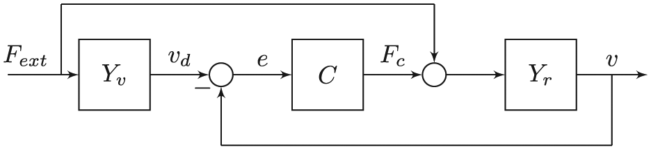
Basic stand-alone admittance control diagram of an uncoupled admittance controlled robot. It shows the measured externally applied force
By making the relation between the measured force and the velocity reference, the virtual model dynamics, consistent with laws of mechanics, simulation of physical dynamical systems is possible (Adams and Hannaford, 1999; Van der Linde et al., 2002).
Admittance control is the opposite, or dual (Adams and Hannaford, 1999; Lammertse, 2004), of the ubiquitous method of impedance control (Hogan, 1985), where forces are applied, either through open-loop or closed-loop control, to the human user after motion is detected. The naming reflects the causality of the used virtual model dynamics. Owing to this dual nature of admittance control and impedance control, they naturally excel at both different ends of the “haptic spectrum” (Adams and Hannaford, 1999; Faulring et al., 2007; Ott et al., 2010; Yokokohji et al., 1996). For admittance controlled devices it is easier to render stiff virtual surfaces and a challenge to render low inertia. It is troubled by dynamically interacting with stiff real surfaces (constrainedmotion) (Adams and Hannaford, 1999; Newman and Zhang, 1994; Surdilovic, 1996). Impedance control, on the other hand, is a better candidate to render low inertia but not to render stiff virtual surfaces. It is troubled by dynamically interacting with low inertia (free motion) (Adams and Hannaford, 1999).
2. Motivation
Although admittance control has been applied successfully in multiple devices (see Section 3.2), an overview of applications, properties, and possibilities of admittance control is lacking. We provide an overview of the development and applications of admittance control. In addition, we briefly recapitulate the notions of stability and passivity of admittance controlled systems. The main contribution of this work is the presentation of an elaborate admittance controller framework and its control scheme that summarizes major contributions from literature and experience, which can be used for controller design and development. Within this framework, we analyze the influence of (1) feed-forward control, (2) force signal filtering, (3) post-sensor inertia compensation, (4) the addition of virtual damping, (5) additional phase lead on the motion reference, (6) motion loop bandwidth, and (7) internal robot flexibility (which in the limit directly relates to series elastic control) on the stability, passivity, and performance of minimal inertia rendering admittance control. Finally, these analyses lead to a set of design guidelines for achieving high-performance admittance controlled devices that can render low inertia, aspiring robust coupled stability. The analyses are focus solely on single-degree-of-freedom (single-DOF), single interface linear-time-invariant (LTI) systems with one-port admittance interaction.
3. Background
3.1. Naming
The name admittance control dates back to 1992 due to the developments of Newman (1992), Gullapalli et al. (1992), and Schimmels and Peshkin (1992). Different names for what is commonly called admittance control can be found in the literature: position-based (Carignan and Smith, 1994; Colbaugh et al., 1992; Heinrichs et al., 1997; Lawrence and Stoughton, 1987; Ott and Nakamura, 2009; Pelletier and Doyon, 1994) or velocity-based impedance control (Duchaine and Gosselin, 2007). It is sometimes interchanged with impedance control (Aguirre-Ollinger et al., 2007; Rahman et al., 1999). In all cases there is the measurement of force that generates a motion control reference or a deviation from such a reference.
Some authors distinguish between motion-based impedance control and admittance control by focusing in the former case on motion tracking and in the latter case on force tracking (Seraji and Colbaugh, 1997; Ueberle and Buss, 2004; Zeng and Hemami, 1997). We choose to use the generic term admittance control for all types of force-to-desired-motion relationships in this work, and recognize the fact that an admittance controller can track both motion and forces simultaneously.
The desired dynamical behavior, the admittance, felt at the “interaction port” where the human interacts with the device, is called by different names: desired dynamics (Carignan and Cleary, 2000), target dynamics (Carignan and Cleary, 2000; Dohring and Newman, 2003), mechanical drive point mobility (Newman, 1992), virtual admittance/environment/model/dynamics (Adams and Hannaford, 1999; Lammertse, 2004), or driving-point dynamics (Colgate and Hogan, 1988). It could also be called the indirect force controller.
Dependent on the form of the desired dynamical behavior, several authors adopt different names for the controller. The term admittance control is used for a inertia simulation (Lammertse, 2004), but also for pure damping (Carmichael and Liu, 2013; Nambi et al., 2011) or generic force to motion simulation (Adams and Hannaford, 1999; Yokokohji et al., 1996). Accommodation control is solely used for pure damping behavior (Newman, 1992; Whitney, 1977). Finally, compliance control is used for pure spring behavior (Zeng and Hemami, 1997). If the controller is to mask only (static) friction effects and keep the same inertia (its natural admittance) as the robot system, Newman and Zhang (1994) proposed the name natural admittance control (NAC).
In this work, we take the aforementioned single analyses, and the major innovations and combine them into a single framework. We use the term virtual dynamics (or virtual admittance) to describe the dynamics we want the device to display to the human, and to refer to the model that is used to calculate a velocity reference for a velocity controller to track. The dynamics that are actually felt by the human will be called the apparent dynamics (or apparent admittance), which preferably approaches the virtual dynamics.
3.2. History and applications
Interaction control gained widespread academic interest after the pioneering work of Hogan (1985) and Colgate (1988) on impedance control and passivity at the end of the 1980s. The first mentions of using a control method very similar to admittance control date back to Whitney (1977), where it was used to respond to hard contact in industrial applications and therefore for indirect force control purposes.
Initially, interaction control was developed for applications such as welding and deburring, where stiff robot position control was highly impractical due to high stiffness and friction of the processed parts (Colbaugh et al., 1992; Schimmels and Peshkin, 1992, 1994; Seraji and Colbaugh, 1997; Whitney, 1977). Accommodation and admittance control were first introduced on retrofitted industrial robots (Colbaugh et al., 1992; Dohring and Newman, 2003; Glosser and Newman, 1994; Maples and Becker, 1986; Pelletier and Doyon, 1994; Whitney, 1977). Ott and Nakamura (2009) exploited a force sensor in the base to increase the safety of the system. Bascetta et al. (2013) use variable admittance control for teaching of industrial manipulators to interact safely during manufacturing.
A patent from Fokker Control Systems (US4398889 A) describes admittance control in flight simulator devices in the field of control loading, starting from 1980. First mentions pHMI come from haptic master devices to render virtual dynamics in flight simulation and later in more generic scenarios (Adams and Hannaford, 2002; Clover, 1999; Strolz and Buss, 2008). In these cases virtual environments with admittance causality could be simulated, allowing more straightforward rendering of constrained motions.
Mentions of active devices capable of safe interaction between human and machines emerged at the beginning of the 1990s (Hogan, 1989; Kazerooni, 1990). Further development of the method led to successful practical admittancebased devices such as the HapticMaster (Van der Linde and Lammertse, 2003; Van der Linde et al., 2002) for generic haptic simulation, the Simodont for the training of dental practice, and Lopes II (Meuleman et al., 2013) for the rehabilitation of human walking, all developed by Moog Inc. (Moog Inc., 2014).
Faulring et al. (2004, 2007) mentioned the use of Cobots with continuous variable transformers (CVTs) to be able to render stiff constraints in an admittance control mode. Other methods employ admittance control in a master-slave setup (Kragic et al., 2005; Lee et al., 2008) for surgery.
Exoskeleton control, used for the upper extremities (Carignan et al., 2009; Huo et al., 2011; Kim et al., 2012; Miller and Rosen, 2010; Yu et al., 2011), is sometimes implemented in multi-DOF admittance-controlled devices to aid in rehabilitation (Carmichael and Liu, 2013; Colombo et al., 2005; Culmer et al., 2005, 2010; Ozkul and Erol Barkana, 2011; Stienen et al., 2010). Rendering low inertia and task-dependent stiffness assist the wearer in making motions with the arm. Owing to the motion-controlled nature of the device, it can switch seamlessly between admittance control and pure motion control. This makes it a good candidate for identification of the human neuromusculoskeletal system dynamics through applied position perturbations, and for switching between automated, reactive, and cooperative tasks, as explained by Stienen et al. (2011).
Several lower-extremity exoskeleton devices use admittance control to render low impedance (high admittance) during the generation of locomotion patterns for rehabilitation purposes (Bortole et al., 2013; Meuleman et al., 2013). For mobile lower-extremity rehabilitation the admittance controller is used to have carts move with the patient with minimal effort (Patton et al., 2008). Other designs are developed for knee recovery specifically (Aguirre-Ollinger et al., 2007; Wang et al., 2009). A method used by Aguirre-Ollinger et al. (2007, 2011) is to use admittance control with acceleration feedback as implicit force control to reduce the inertia of the lower leg of the human to facilitate knee recovery (Aguirre-Ollinger et al., 2012). Rehabilitation of the ankle with admittance control is described by Saglia et al. (2010).
Admittance control for end-point interaction is mainly used for power amplification or load reduction (Colgate et al., 2003; Kazerooni and Guo, 1993; Lecours et al., 2012; Surdilovic and Radojicic, 2007) and the masking of unwanted dynamical effects in industrial applications. In these cases the heavy-load-bearing capabilities of large and strong devices can result in substantial power amplification of a human user.
Special cases of admittance control can be found for interaction with humanoids (Li et al., 2012; Okunev et al., 2012), anthropomorphic arms and hands (Yamada et al., 2013), aerial vehicles (Augugliaro and D’Andrea, 2013), and mobile carts (Wang et al., 2015).
Furthermore, learning and adapting admittance control schemes have been implemented (Gullapalli et al., 1992). Adaptive models, time-varying parameters, or neural networks are used to optimize the interaction between the device and the human towards some objective (Dimeas et al., 2013; Prabhu and Garg, 1998; Yu et al., 2013).
3.3. Design challenges
Owing to the velocity or position controlled nature of many admittance controlled devices, it is straightforward to create stiff or dissipative haptic constraints to assist in cooperative human–robot tasks. When the human is not supposed to be constrained, the device should have high admittance (i.e. low impedance). Preferably, the apparent admittance should be higher than the natural admittance of the inert, heavy, and dissipative robot.
Infinite admittance, or zero impedance, over the complete frequency range is impossible to achieve on an admittance controlled device due to division by zero in the force–velocity relationship. A common approach is to have the virtual dynamics be a pure virtual inertia (Aguirre-Ollinger et al., 2007) that is as “low as possible,” while retaining stability when coupled to the user. The pure virtual inertia assures low impedance for low frequencies, attenuation of high frequencies, and non-dissipative behavior. The low virtual inertia admittance approach is the same as high integral indirect force control with an inner velocity-control loop. The integral force gain is the reciprocal of the virtual inertia. Effectively, the low virtual inertia generates a force controller that attempts to minimize the interaction force between device and the user.
A problem with this method (further described in Section 5.3) is that when lowering the virtual inertia, the robot becomes unstable when in contact with stiffened human limbs or stiff environments. To reduce the apparent inertia while keeping safe and stable interaction behavior is therefore a challenge for admittance control.
Owing to the high bandwidth of the inner motion-control loop, the admittance controller can achieve significant masking of nonlinear static friction effects inherent to the device itself (Newman and Zhang, 1994). The drawback of such a high motion-control bandwidth is the sensitivity of the controller to drive-train backlash and flexibility. Drive-train backlash and flexibility can result in unstable position-velocity limit cycles (Aguirre-Ollinger et al., 2007).
3.4. Admittance control in perspective
3.4.1. Admittance control as a form of teleoperation
Admittance control can be seen as a form of indirect force control (Zeng and Hemami, 1997), or as a specific case of a bilateral teleoperation controller. The latter fits the framework of the 4C Controller, as popularized by Lawrence (1993) and Hashtrudi-Zaad and Salcudean (2001). In this case it comprises a virtual admittance slave with possibly added virtual environment, without any communication delays. In this framework it is called the position–force architecture, reflecting the human causality instead of model causality. Attempting to simulate any “virtual slave” system on an admittance controlled setup is similar to designing a master–slave setup with dissimilar master–slave dynamics and kinematics.
3.4.2. Admittance versus impedance control
The main difference between admittance control and impedance control is that the former controls motion after a force is measured, and the latter controls force after motion or deviation from a set point is measured (Lammertse, 2004).
Impedance controlled devices are commonly used for manual haptic and teleoperation displays. Admittance control is used more often in larger non-backdrivable high-friction devices that are of the full-body type (e.g. wearable robotics) and heavy-duty type (e.g. industry). This difference is mainly due to the ease of designing adequately performing impedance controlled devices withopen-loop force generation. It circumvents the need of using a force sensor, which is generally expensive and sensitive to drift and temperature change, and does not demand stiff mechanics of the robot as is preferred for a closed-loop force controlled system. A drawback of such an impedance control method is the disturbing “feel” of the remaining parasitic dynamics and friction effects of the device itself (Adams and Hannaford, 1999). Therefore, these impedance devices are commonly designed to be lightweight and to have low friction. If the impedance control force generation is open loop, the device is highly forgiving to backlash and drive-train flexibility.
If explicit force control is used in the impedance controller, i.e. impedance control with force feedback (Adams and Hannaford, 1999; Carignan and Cleary, 2000; Faulring et al., 2007), the system’s parasitic dynamics are highly suppressed. However, low-frequency resonant modes and backlash will destabilize the system (Adams and Hannaford, 1999). The closed-loop control of force in impedance control, and the closed-loop control of motion in admittance control, result in better approaching of the virtual dynamics. Possible non-collocation of force sensor and actuator limits the achievable force control bandwidth in impedance control. This is less of a problem in admittance control, since the actuator and velocity sensor are usually collocated, although such internal flexibility allows for less robust coupled stability and reduced approximation of the virtual dynamics. The range of achievable apparent dynamics or z -width (Colgate and Brown, 1994) is higher for admittance control than for impedance control (Adams and Hannaford, 1999; Faulring et al., 2007).
4. Stability and passivity
In contrast to a motion servo, a system that focuses on stable physical interaction aspires several kinds of stability (Colgate and Hogan, 1988), of which the last will be discussed separately.
Uncoupled stability, when the device is “free,” not being in contact with a human.
Contact transition stability, when transitioning from being free to being in contact.
Coupled stability, when the device is and stays in contact with a user or environment.
In practical cases the admittance controlled robot will make contact, or will already be in contact with a human, an object or the fixed world. The possible making or breaking of contact, is a contact transition, which can lead to non-trivial transition or switching instability (Liberzon, 2003). However, we neglect the transitioning stage in our analyses, assuming a robotic device that has been held by, or attached to, a human user for sufficiently long time, or has its controller software started while already fully in contact or when fully uncoupled.
4.1. Coupled stability
A human and machine being in contact, exchanging mechanical power or exerting forces bilaterally, behave as a single coupled system as shown in Figure 2. Coupling stability is non-trivial, since two separately stable systems can exhibit coupled instability (Colgate, 1988), or an unstable robot system could become stable after coupling it to a human user.
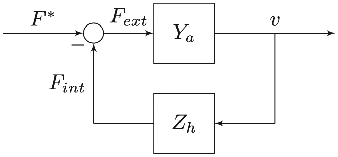
Interconnection of admittance controlled robot that has apparent admittance
The coupling of an admittance controlled device with
4.2. Robust coupled stability: energy passivity
The analysis method related to energy passivity (Raisbeck, 1954) made its way from electrical network coupling stability to robot–human and robot–environment interaction. It allows the use of a similar argument to guarantee stability of robots during interaction (i.e. coupling) with all possible energetically passive environments. The situation where the robot interacts with a human user is different, in the sense that the human user can exhibit non-passive dynamical behavior (Dyck et al., 2013). However, from everyday experience we know that the interaction of humans with passive objects is stable. Therefore, as long as the controlled robot’s apparent dynamics are energetically passive, the interaction between robot and human will be stable.
Energetically passive behavior of the apparent dynamics of the controlled robot, together with good performance, form therefore a design “goal” to aim for, since it puts the responsibility of interaction stability with the human. Passivity conditions are useful during controller design, and are investigated in the remainder of this work.
4.2.1. Definition
The definition of an energetically passive one-port system is that it cannot deliver more energy than what was put into it (Colgate, 1988); i.e. for mechanical systems it would be required that
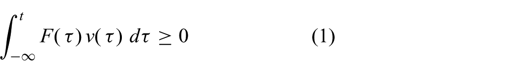
where F and v are power-conjugated force and velocity inputs or outputs of a mechanical system of either admittance or impedance causality. If the apparent dynamical behavior of the robot during free motions is designed to behave like a passive system in accordance with Equation (1), stability is guaranteed for any combination of the passive robot coupled to another passive system.
Colgate (1988) described a method to assess passivity in the frequency domain for LTI systems. A single-DOF LTI controlled robot, in our case the uncoupled apparent dynamics
any imaginary poles of
The first condition we usually conform to in stable motion control. The combination of the second and third conditions is commonly referred to as the positive real condition (Colgate, 1988), which provides useful design guidelines. Following Dohring and Newman (2003), the positive real condition for systems without time delay reduces to the demand that
A consequence of the positive real condition is that, the apparent dynamics
4.2.2. Practicality
Several authors suggest that enforcing passivity is too conservative for human–machine interaction (Adams and Hannaford, 1999; Buerger and Hogan, 2006; Haddadi, 2011; Hashtrudi-Zaad and Salcudean, 2001; Willaert et al., 2009). This is mainly due to the fact that the human interaction impedance in practice is bounded. Therefore, aiming for coupled stability with any human limb that can be infinitely stiff, infinite in inertial mass, or infinitely dissipative, is conservative.
A controller design method used by Adams and Hannaford (1999) to take finite human impedance into account, is to absorb the maximal and minimal human admittance into the robot’s apparent admittance. The new robot admittance is coupled to an abstract passive human impedance that is allowed to take on any value. This allows for application of the positive real condition for design, while still accounting for the limited human impedance range.
Investigations into the limited impedance ranges of the human arm are also discussed by Buerger and Hogan (2006, 2007). The coupled stability problem is consequently handled as a robust control problem with known parametric uncertainty in the human impedance parameters. A constrained optimization method is used to find controller gains that achieve good apparent dynamics and guaranteed stability within a limited human impedance range.
Haddadi (2011) developed a passivity-based robust stability method that is less conservative than the approached described above. Rules and visual aids are developed to incorporate bounds of the human or environment impedance for less-conservative guaranteed stability conditions, with a better trade-off between stability and performance.
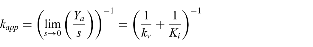
4.3. Ez-width
Passive behavior of a controlled robot might not always be achievable due to controller choices or due to unwanted poor dynamical performance when the robot is behaving passively. If by controller design the apparent dynamics
In this work, the ez-width is used to see in what range the human limb stiffness and damping can be if we depart from the wish for (strict) passivity of the apparent dynamics
It should be noted, however, that the usefulness of ez-width diagrams relies heavily on the major assumption that a second-order passive quasi-linear mass–spring–damper model is sufficient to describe neural feedback-controlled human limb behavior. Although several studies show that for certain tasks this assumption holds (e.g. Hogan, 1989), for other tasks or robot admittance it does not (Dyck et al., 2013). Therefore, the ez-width diagrams only show best-case interaction scenarios where the human would behave fully passively. This assumption could be violated during more realistic real-world tasks, resulting in reduced effective ez-width.
5. Admittance control model
In this section, a generic electromechanical set-up and a control model are presented to explain several of the observed instability and performance effects. The control model incorporates ideas from literature and from our experience. The goal of this section is to give the reader an introduction to a naive admittance controller design to expand upon with the ‘guidelines’ discussed in Section 6.
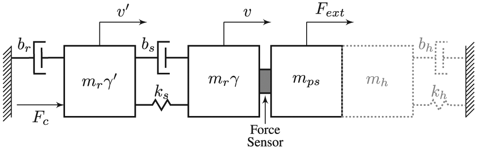
5.1. Physical setup
A schematic admittance controlled device is shown in Figure 3. An actuator generates mechanical power by the supply of electrical power through a controlled current or applied voltage. Such an actuator is commonly an electromechanical motor, although hydraulic actuation has been implemented successfully (Heinrichs et al., 1997). These actuators usually impose forces on the mechanics of the device, which consists of a drive train, moving parts and robotic links. Close to the interaction point a force sensor measures the interaction forces with the user. This sensor is usually non-collocated with the actuator.
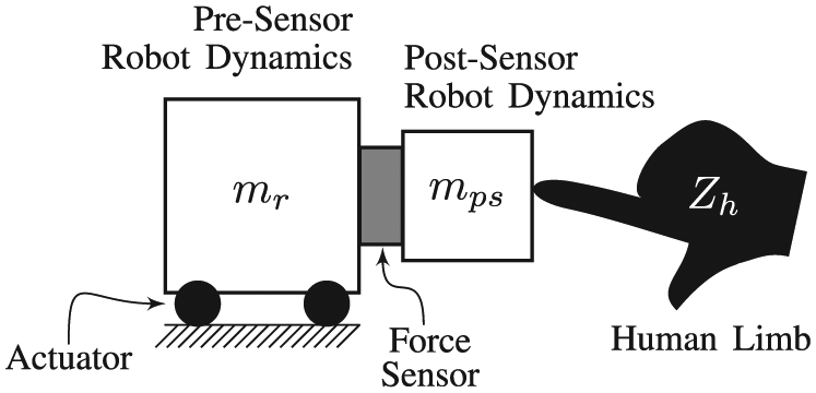
Generic electromechanical system overview of an admittance controlled device. An actuator moves all mechanics (robot inertia
A force sensor has non-zero inertia, and usually a tool (for industrial applications), handle (for manual interaction) or cuff (for exoskeleton-like applications) is attached to the sensor. It will measure these post-sensor dynamics during motion of the pre-sensor system as an impedance effect. These post-sensor dynamics can be thought of as the known time-invariant impedance of the interaction dynamics, and is preferably solely inertial in nature. These post-sensor dynamics do not include the user’s dynamics. We therefore deem the user’s impedance to be the unknown impedance
5.2. Admittance control diagram
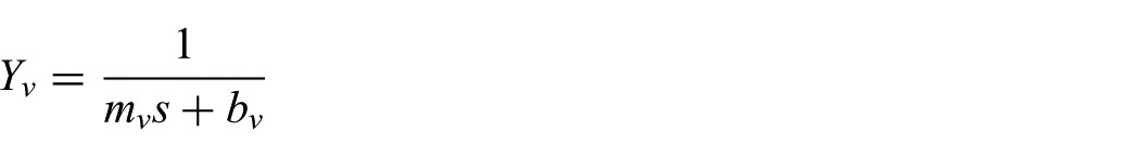
The stand-alone apparent dynamics
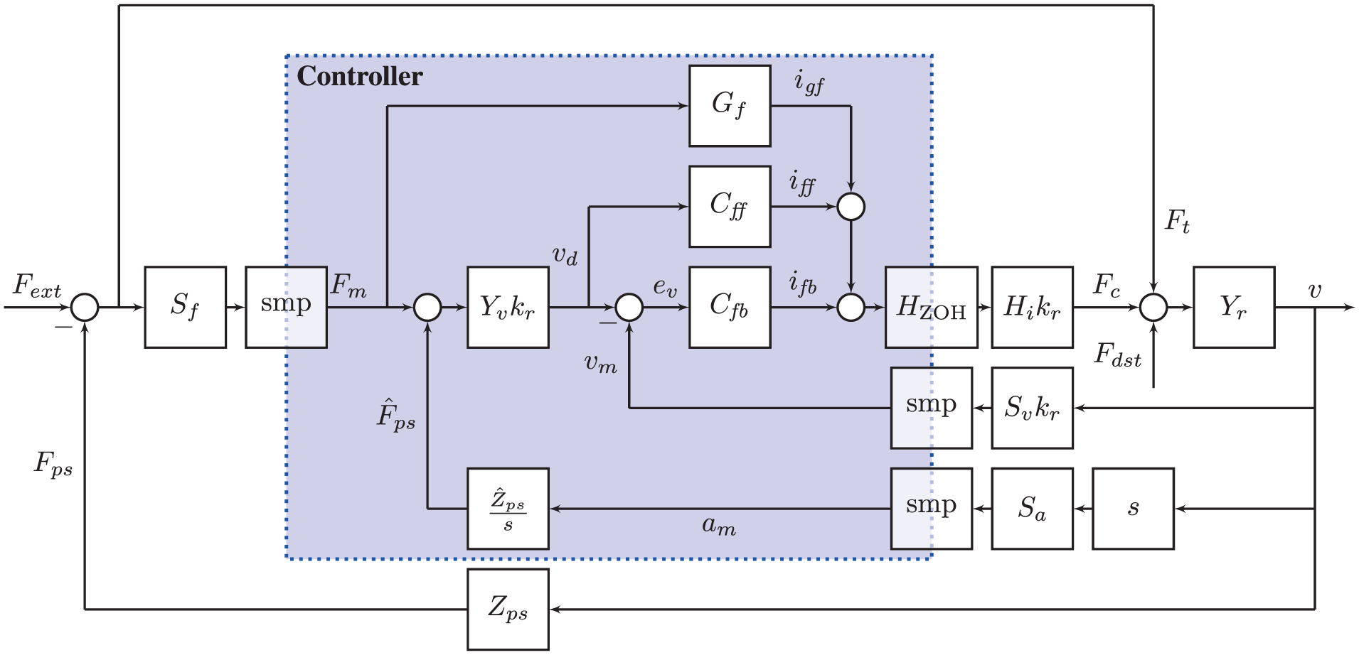
Expansion of the apparent robot dynamics
The total control diagram is composed of several subsystems that will be discussed in the following paragraphs. Dependence on Laplace variable s is mostly omitted for readability and used symbols are explained in Appendix 1.
5.2.1. Forces on the system
Externally applied force (
5.2.2. From measured force to desired velocity
The signal is consequently sampled (
5.2.3. Control and actuation
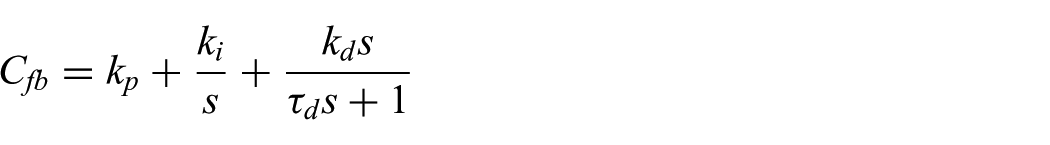
The velocity controller outputs a desired electrical current to be imposed on the actuators by the current controller. The velocity controller consists of a feed-forward (
All reference current values from the force-amplification, feed-forward, and feedback control (
The controlled current generates a motor control force (
5.2.4. Resulting motion and impedance effects
The robot’s resulting motion is due to the sum of these forces. This motion is measured by a velocity sensor or observer (
5.3. Control model
We are interested in a simple model that can explain instability when in contact with stiff human limbs or environments. We call this model the baseline model, with which we can compare performance of possible improvements. It constitutes a naive admittance controller with feedback control only and virtual dynamics as in Figure 1. The robot constitutes a rigid-body mass with some dissipation, and is shown in Figure 5. The apparent dynamics of this baseline system is denoted by
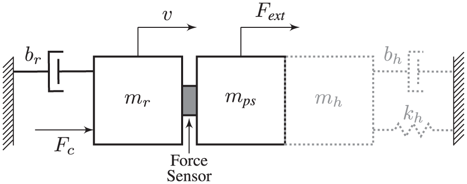
Schematic view of a rigid robot. An external force
This baseline model is derived from the elaborate model in Figure 4. We assume ideal sensors, such that (
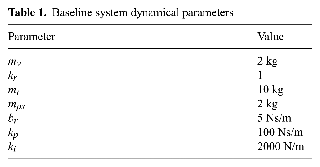
Baseline system dynamical parameters
The equation of motion of the system in Figure 5, omitting the human impedance, absorbing any external force (either from human impedance or extraneous force) into

with

The controller equations for this baseline model for virtual dynamics of inertial form (virtual inertia

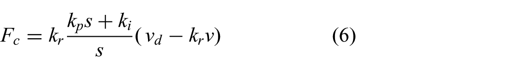
with
5.3.1. Uncoupled stability
For positive choices for all parameters, the apparent dynamics created by Equations (3)–(6) has three poles: one valued zero from the purely inertial virtual dynamics
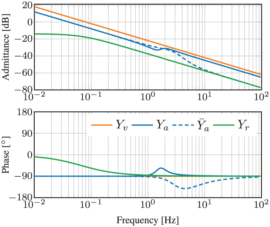
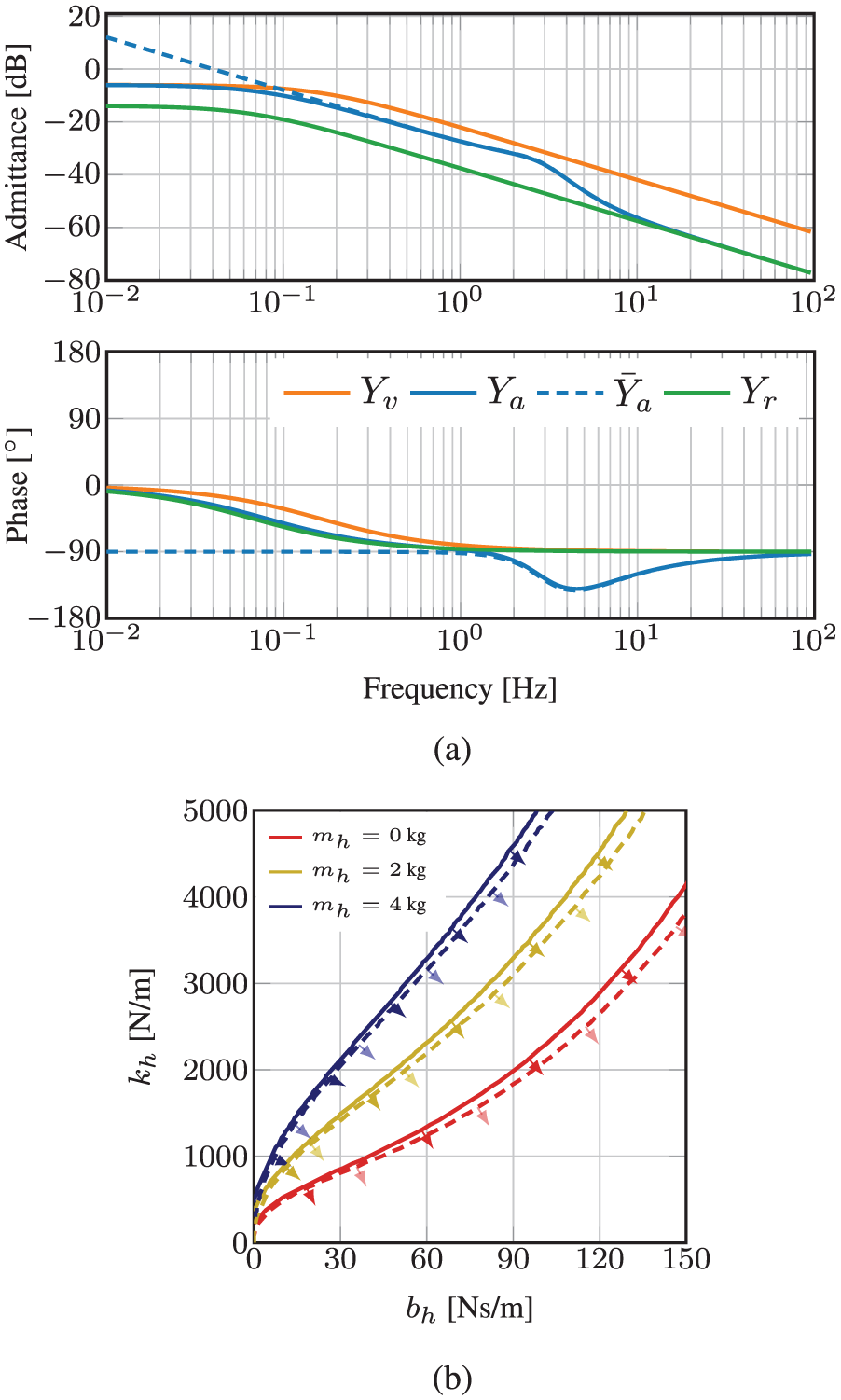
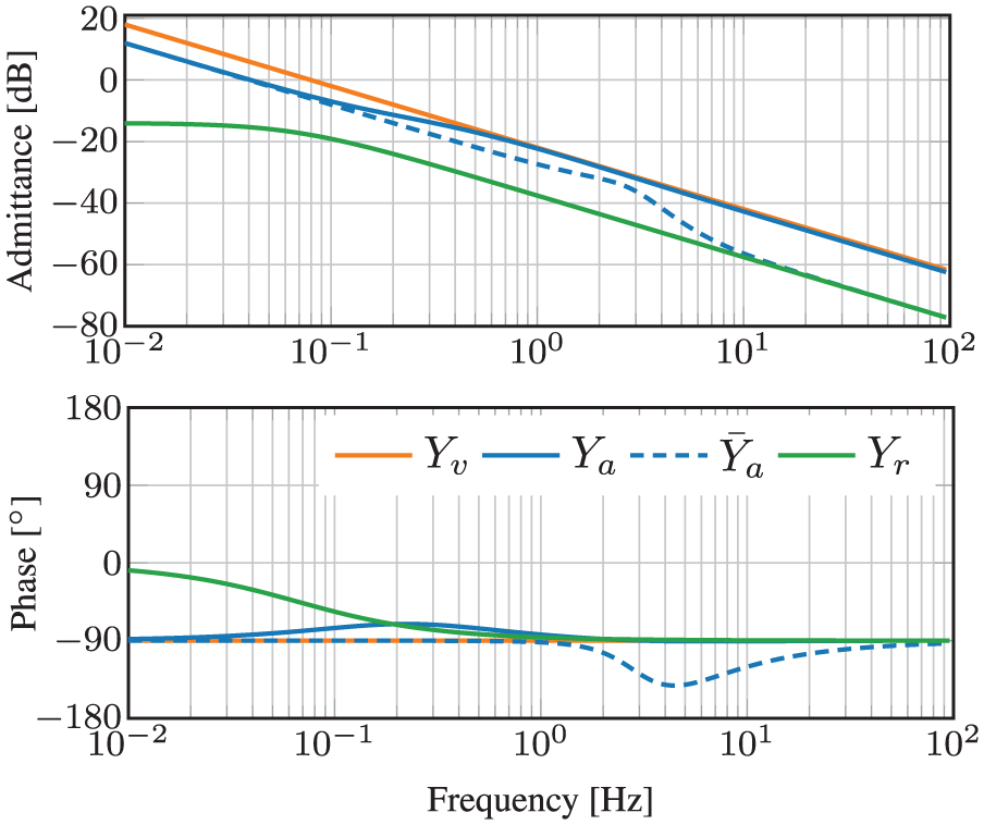
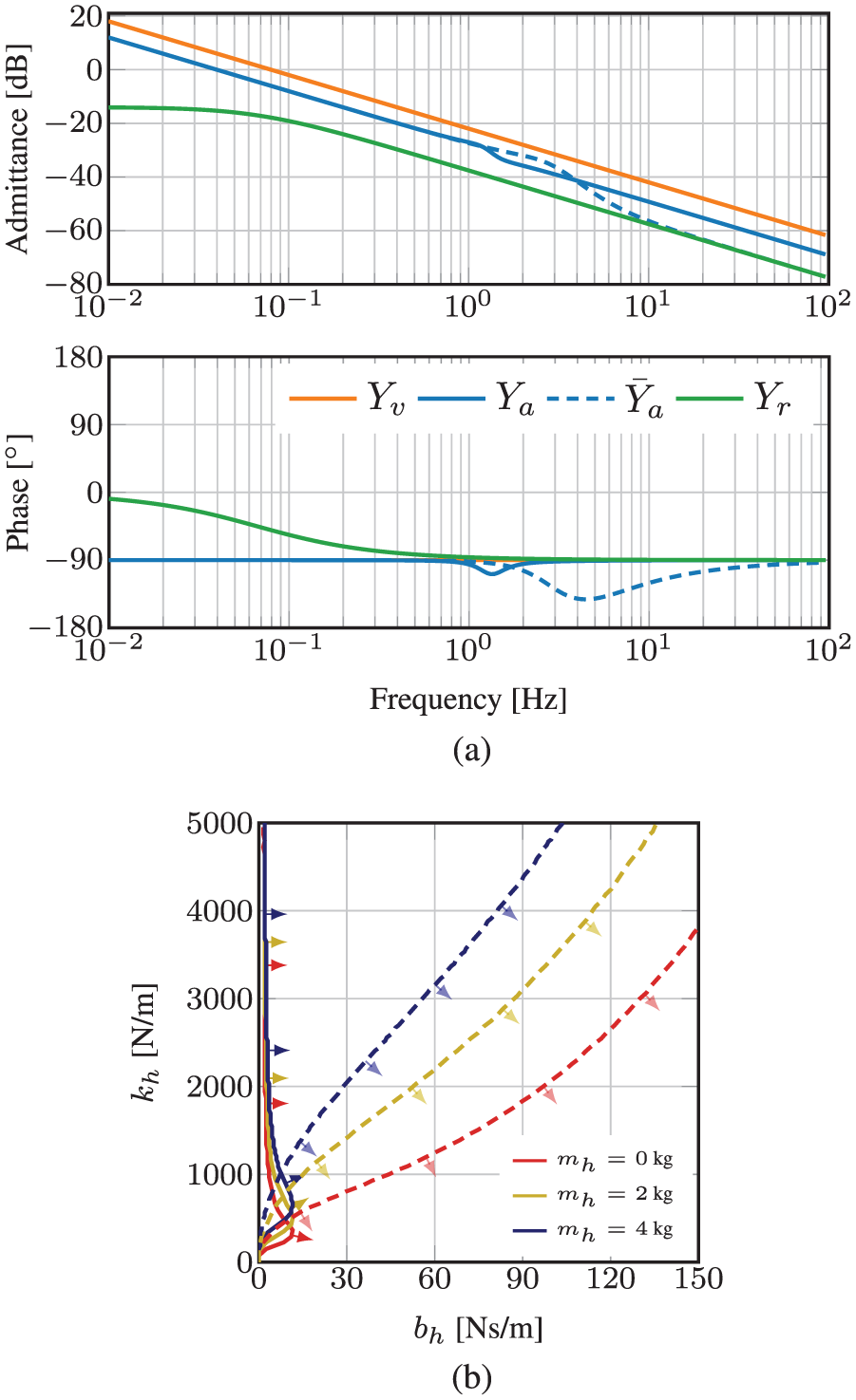
In Figure 6a is shown that the baseline apparent admittance
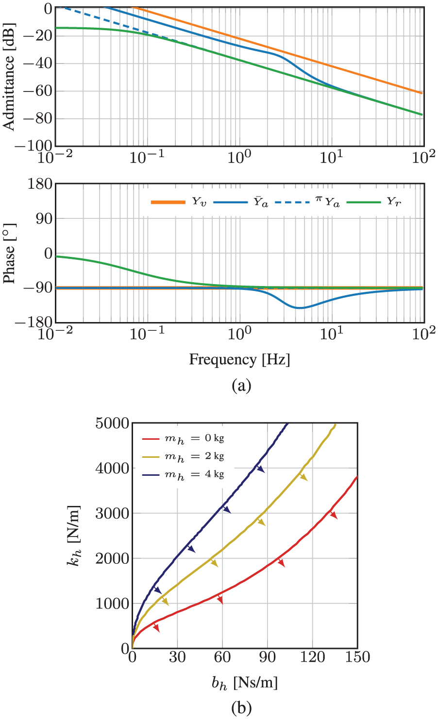
Behavior and performance of a typical admittance controlled system. (a) Bode plot of the uncoupled system: apparent dynamics
5.3.2. Passivity of the uncoupled apparent dynamics
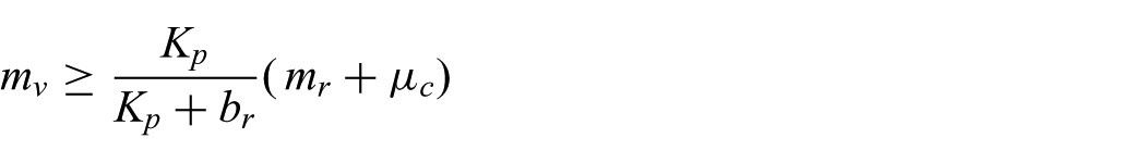
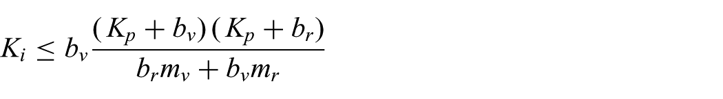
Passivity of this robot is guaranteed if and only if

with
5.3.3. Coupled stability
The uncoupled baseline system with parameters described in Table 1 is not passive and will have finite ez-width, when coupled to a passive human limb, as is shown in Figure 6b.
All the stability boundaries in Figure 6b have in common that they pass through the origin, for any human limb inertia. This shows that admittance controlled systems would never be stable for interaction with pure springs, or pure spring–mass combinations. This is something that is not observed in practice, because all human limbs and realistic mechanical environments have some form of energy dissipation. The upward slope of all curves through the origin shows that adding limb damping yields a decent “stiffness margin” and stable interaction.
5.4. Virtual damping and stiffness behavior
Naive admittance controllers can more straightforwardly render pure virtual damping (i.e. accommodation) and pure stiffness effects passively with decent performance. This is illustrated in Figure 7a and Figure 7b. For low frequencies the apparent admittance approaches the virtual admittance well for both accommodation and stiffness control. Above the feedback controller bandwidth, the apparent admittance becomes inertial in nature due to the robot’s intrinsic dynamics.
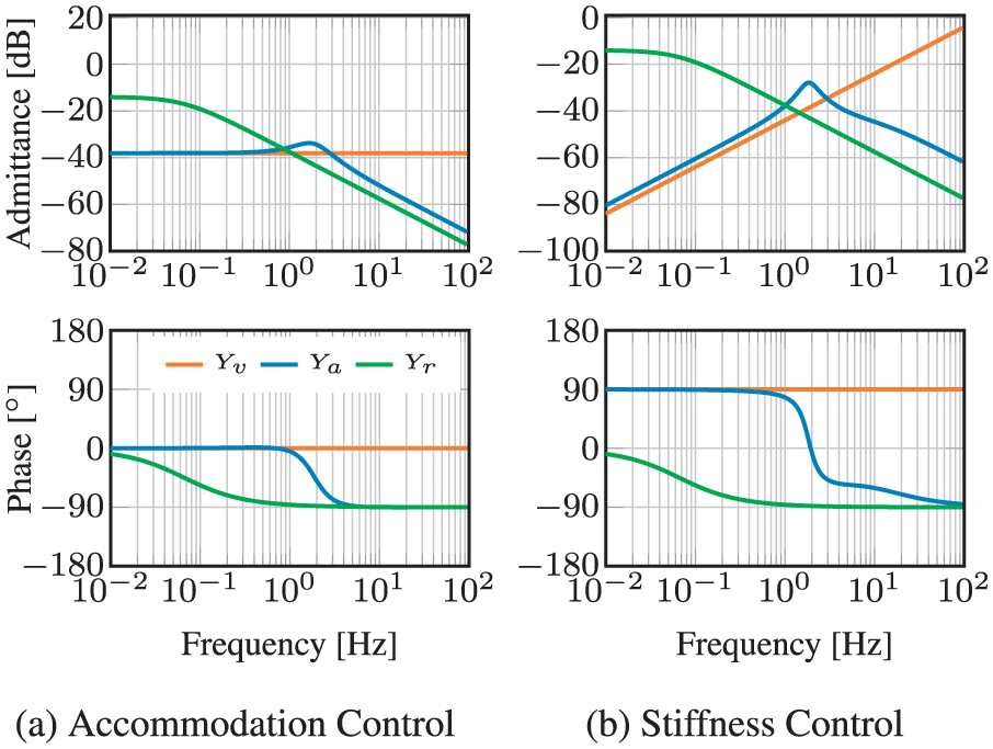
Admittance control apparent dynamics
If in Equation (4) the virtual dynamics are replaced by
This shows again that
If in Equation (4) the virtual dynamics are replaced by
or two springs (the integral/position gain and the virtual stiffness) in series, as can be seen in Figure 7b. The apparent stiffness differs slightly from the virtual stiffness due to finite integral controller gain
5.5. Virtual element combinations
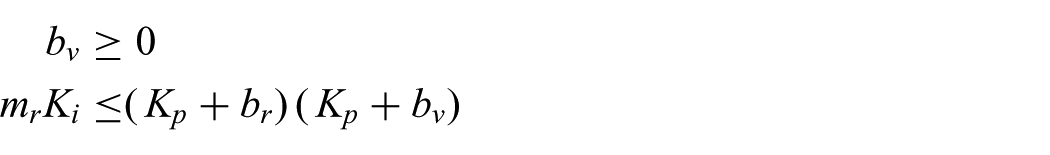
For combinations of mass–spring–damper elements in the virtual dynamics, the passivity conditions become combinations of the conditions presented in the previous sections. This leads to upper and lower limits of robot and controller parameters that become difficult to interpret as design guidelines in some cases. The effective behavior of these passivity conditions, and what they effectively teach us, is shown in Table 2. Note that the mass–damper combination is also discussed in more detail in Section 6.4.
Conditions
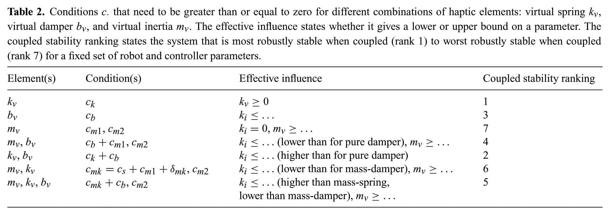
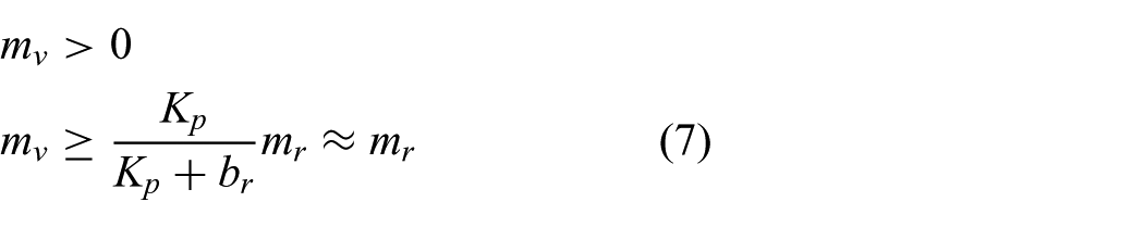
As a rule of thumb it can be stated that if virtual mass is used, the condition in Equation (7) is invariant to addition of other elements. In addition, the conditions for a spring–damper combination add directly (therefore reducing the passivity of a pure spring), but the mass–spring combination acquires an extra addition to the passivity condition.
Table 2 also gives a coupled stability robustness ranking from 1 (the best) to 7 (the worst) showing for a fixed set of controller and robot parameters which virtual admittance makes the robot “most” passive.
Note that the virtual mass–spring–damper case is the only combination that also has a non-trivial uncoupled stability requirement related to an upper limit on
6. Guidelines for minimal inertia
In Section 5.4 it was shown that pure damping and stiffness are readily rendered passively by the robot. Therefore, we focus on the challenge of rendering low system inertia. We expand the naive model from Section 5.3 to incorporate and analyze additions to the control diagram that are shown in Figure 4 and were discussed in Section 5.2. We use the passivity criterion for the uncoupled system, the ez-width of the system coupled to a passive second order system, disturbance rejection and admittance tracking performance (i.e. how well the apparent admittance matches the virtual admittance) to draw conclusions about the feasibility of certain design choices. We will always compare a change in design or model to the “baseline” controller from Section 5.3, and attempt the same inertia reduction of a factor five from 10 to 2 kg.
From this analysis follows a set of guidelines that is presented here in random order. The derivation of the apparent dynamical behavior, the uncoupled stability conditions and positive real conditions for all the guidelines are shown in Appendices 2 and 3.
6.1. Guideline 1: Use feed-forward control
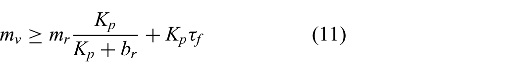
If the robot controller can be used in torque (or current) control mode it is beneficial to use feed-forward control. Feed-forward control can be applied in the form of force gain (
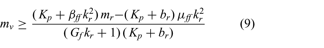

By setting
For high transmission ratios, the passivity condition in Equation (9) reduces to
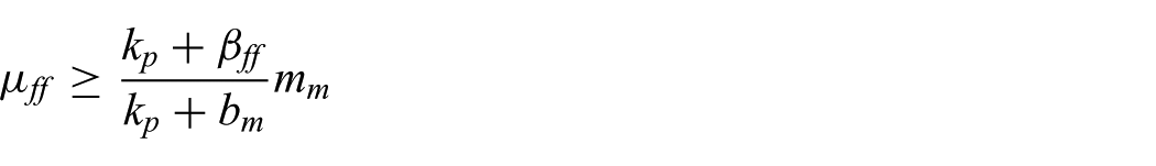
This shows that only with feed-forward does high transmission actually help in achieving some passive low virtual inertia.
The use of feed-forward increases both the ez-width and improves the admittance tracking performance for high frequencies above the velocity controller bandwidth. As is shown in Figure 8, the admittance can be made passive (the ez-width becomes infinite), while approaching the virtual admittance much better at high frequencies than the baseline system
Comparing the use of feed-forward control (
Without any feed-forward (i.e.
6.2. Guideline 2: Avoid force filtering
It is tempting to low-pass filter force sensor measurements to reduce effects of noise or aliasing that cause random motion of the robot. This should be avoided if the virtual admittance is purely inertial (i.e.

with
Setting
Filtering will therefore reduce ez-width (see Figure 9b for an extreme case of low-pass filtering) and limit high-frequency apparent admittance performance (see Figure 9a). This is not problematic for n=1 with accommodation control, or n=2 for stiffness control, which will both effectively become admittance control due to the extra pole(s) of the filter (see Appendix 3).
Influence of low-pass filtering the measured force on system performance and interaction stability. (a) This bode plot shows a system with force filtering (
If filtering is inevitable, e.g. for anti-aliasing, then the filter bandwidth should be as high as possible and the filter order as low as possible.
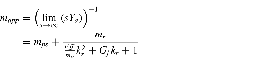
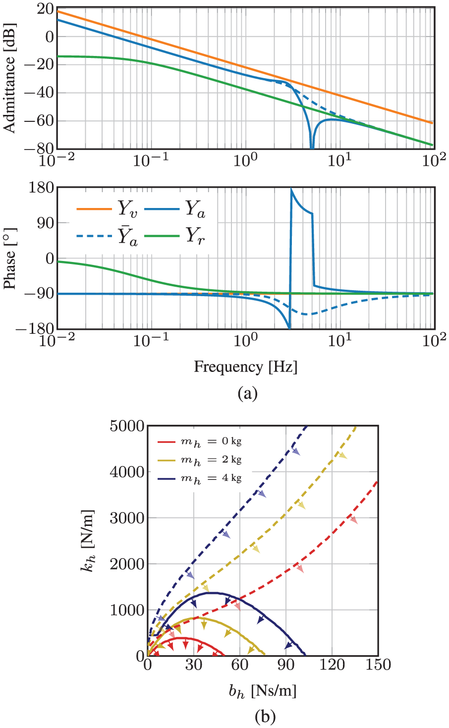
6.3. Guideline 3: Compensate post-sensor inertia
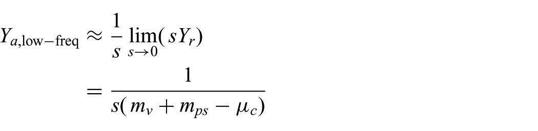
Post-sensor dynamical effects are not reduced or masked by the basic admittance controller (Section 5.3), or by feed-forward control (Section 6.1). The post-sensor inertial effects can be compensated in the low-frequency range by performing post-sensor dynamics compensation (in impedance form) with a compensation inertia
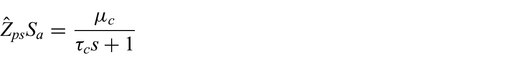
This improves the performance, because indeed we achieve the following apparent inertial behavior at low frequencies:
If
Influence of post-sensor compensation on system performance and interaction stability. (a) This bode plot shows a system with post-sensor compensation (
This method, however, reduces ez-width (see Figure 10b). The passivity condition in Equation (7) changes to (assuming
where
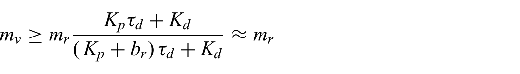
In accordance with Aguirre-Ollinger et al. (2011, 2012) this method can also be used to effectively give the robot negative inertia. This will reduce the inertia of the object or human limb attached to the robot. For this to work,
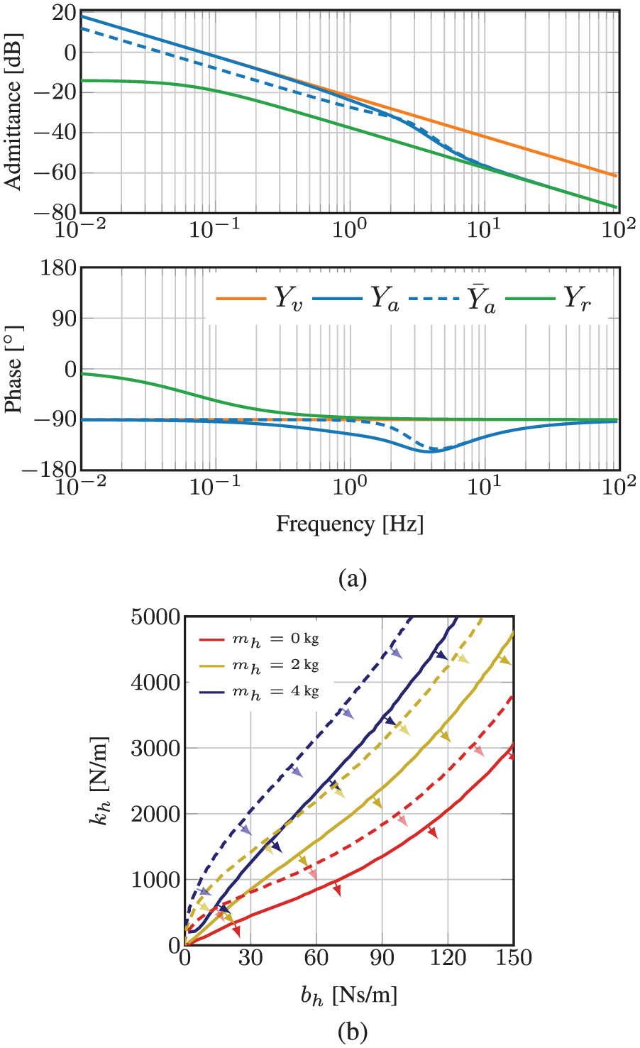
6.4. Guideline 4: Use some virtual damping
Virtual admittance of inertial form can in most applications be changed to a combination of inertia and a small amount of damping
The small amount of damping (
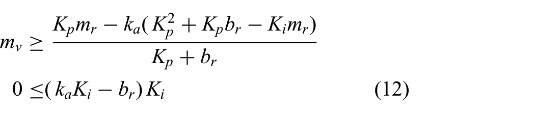
The passivity conditions in Equation (8) changes, when adding some virtual damping, to
Passivity condition in Equation (7) is left unaltered, i.e. adding some virtual damping will not allow for lower
Influence of adding virtual damping on system performance and interaction stability. (a) This bode plot shows a system with some virtual damping (
Figure 11b shows that ez-width becomes larger when adding some virtual damping. A minor penalty for using damping is the dissipative nature, impeding motion.
6.5. Guideline 5: Modify the velocity reference
It is common that industrial robots with “black box” PI velocity control (or equivalently PD position control) are retrofitted with an admittance controller. In that case, adding feed-forward (guideline 1) is not possible, and some other way has to be found to obtain better admittance tracking and good ez-width.
It is possible to change the virtual admittance and add some form of acceleration feed-forward with gain

with
The passivity conditions in Equations (7) and (8) change to
This complex looking condition gives us some advice: (1) use a robot with minimal inertia
Influence of a system with extra phase lead (
6.6. Guideline 6: Increase velocity loop bandwidth
Many passivity conditions in the aforementioned guidelines demand low
6.6.1. Add differential velocity control
An additional method to increase the velocity control bandwidth is to use a PID velocity (PDD2 position) controller (Aung and Kikuuwe, 2015). The feedback controller is augmented with differential gain
To be a proper and implementable transfer function, differentiation is band-limited by the low-pass filter. Unfortunately, the passivity condition from Equation (8) remains unaltered. The passivity condition from Equation (7) becomes
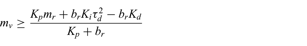
with
Band-limited differential control action has little effect on the passivity conditions, and it cannot make the system passive with
However, as expected, adding a band-limited differential velocity controller assists in achieving the better high-frequency approach of the virtual admittance, as is shown in Figure 13a. Adding differential gain also increases the ez-width drastically, as is shown in Figure 13b. This behavior is due to the introduced zero in the transfer function due to the differentiation, and now we can choose the location of the new pole location that was introduced by the low-pass filter.
Influence of differential velocity control on system performance and interaction stability. (a) Bode plot to compare a system with band-limited differential control (
6.6.2. Reduce time delays
Another method to achieve higher-velocity bandwidth in practical setups is to reduce any additional phase lag due to DA conversion (ZOH) or current controller delays. The ZOH dynamics, for a system with sample time
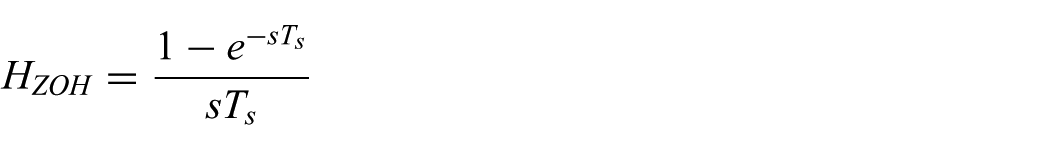
which has
6.7. Guideline 7: Optimize for robot stiffness
If we consider a flexible robot with a low-frequency resonant mode (below the controllers’ Nyquist frequency), we can model this as two inertias sharing a fraction
Schematic view of a flexible robot, or a system with series elastic actuation. The robot now consists of two inertias
According to Colgate and Hogan (1989) the inertia cannot be passively reduced to any inertia smaller than
The performance with a high-frequency mode is acceptable (see Figure 15a). The ez-width is sensitive to

The influence of having a system with finite internal stiffness on system performance and interaction stability (a) This bode plot shows a system with finite stiffness (
7. Discussion
Naive haptic admittance controllers that use only feedback control achieve passivity with good approach of the intended dynamics, when rendering pure virtual stiffness or pure damping. However, such controllers have difficulty rendering pure inertia lower than the original device inertia. This is inconvenient, since the admittance control paradigm is commonly used to attempt inertia reduction of bulky devices. The analyses in this paper, our experience, and reports in literature show that attemptedinertia reduction leads to coupled instability. With a feedback-only velocity controller, admittance controllers become unstable when the device is firmly held by humans (e.g. for cooperative industrial tasks or haptic displays) or when it is attached to limbs (e.g. for rehabilitation devices). However, completely avoiding feedback control is infeasible, since it is required to suppress unwanted disturbances from external forces and friction forces.
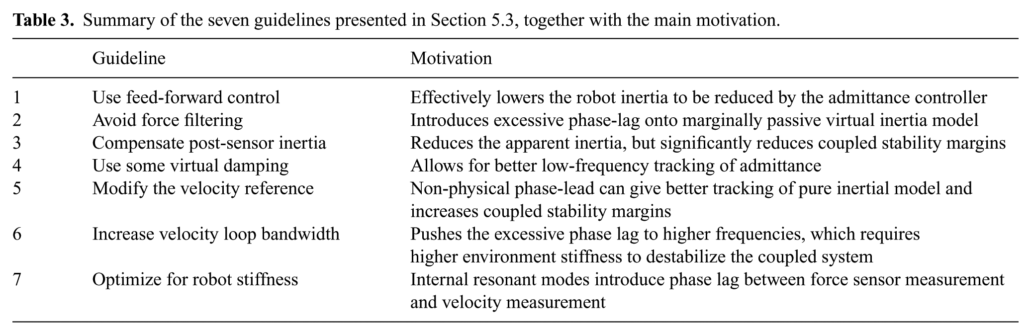
The guidelines presented in this work, summarized in Table 3, propose several solutions to this coupled instability problem when rendering virtual inertia lower than the device inertia. The goal of these guidelines is to simultaneously (1) achieve a better approach of the apparent dynamics to the intended virtual dynamics, and (2) ensure robust coupled stability in the sense of passivity. The guidelines give a qualitative description of how to design key parameters of the mechanical system and control system. These were derived from the fact that the design has to be close to passivity, but also approach the intended dynamics properly with sufficient disturbance rejection. We did not discuss proper controller design (i.e. choices for tuning feedback gains). Any objective in terms of robustness or optimality could be used for determining feedback controller gains, as long as these are within uncoupled stability bounds, and interaction stability bounds given in this work. The ez-width or passivity bounds should be used as optimization constraints during such controller design.
Summary of the seven guidelines presented in Section 5.3, together with the main motivation.
Using the presented framework for designing admittance controlled systems has several limitations. We derived most of the guidelines from an idealized stiff and single-DOF robot. In multi-DOF robots, energetic coupling between nonlinear DOFs could result in instability effects absent in single-DOF analyses. A dynamical model with distributed mechanical compliance might be more useful in practical cases. However, the analysis for a system with a single resonant mode leads to qualitatively non-informative and complex conditions for passivity, uncoupled stability and interaction stability. For a distributed flexible model this would be even more so. Nevertheless, while the conditions might seem complicated, they could be incorporated in design software.
In practice, velocity measurements required for velocity control can be performed by tachometers (EMF-based) or gyroscopes. The more common alternative of numerical differentiation of joint position encoder signals with high spatial resolution leads to quantized and noisy estimates of joint velocity. Such a noisy estimate result in a noisy or grindy feel when interacting with the robot. Low-pass filtering this quantization noise results in unwanted resonance in the PI velocity controller’s feedback loop and jeopardizes passivity. Therefore, estimation methods that use optimal integration of joint position measurements, joint acceleration estimations and a model of the device could give a joint velocity estimation with low phase lag and a high signal-to-noise ratio.
However, measuring or estimating the robot accelerations, also required for guidelines 3 and 6, can be difficult in practice. We have added first-order low-pass filters in the analyses to indicate limited sensor bandwidth observed in practice. Accelerometers output noisy signals, resulting in a noisy feel of the device during interaction. Other acceleration estimation methods, such as double numerical differentiation of joint-encoder measurements yield heavily quantized and noisy estimations as well. Possible state observer models together with optimal sensory integration could aid in obtaining an optimal estimation of the acceleration. Note that guidelines 1 and 5 do not need acceleration measurements. These use the accelerations from the virtual dynamics, which are derived from the force measurements.
The analyses in this work focused mostly on the influence of isolated parameter changes. Coupled parameter changes, for example by using feed-forward control and a low-pass filter on the force concurrently, were not discussed. Applying two guidelines, or changing two system variables could show unexpected interaction.
We briefly discussed the influence of ZOH and time-delay effects on passivity properties. Using discrete time sub-models for the feedback controller, virtual dynamics and possible state estimators might give slightly different and more realistic passivity conditions. Nevertheless, since haptic devices usually use fast sampling frequencies above1,000 Hz, we assume that the found guidelines are valid.
The post-sensor effects analyzed were assumed to be purely inertial. In practice, we notice that post-sensor backlash and flexibility leads to unwanted limit cycles. Whether this behavior is to be expected from the apparent dynamics in combination with coupled post-sensor dynamics, or exhibit a different form of instability, has to be further analyzed.
Footnotes
Appendix 1: Notation and suffixes
Appendix 2: Full system transfer function
The full transfer function for the system shown in Figure 4 is given by
with
The disturbance force influence is given by
In its most elaborate form, the following subsystems are used (see Appendix 1 for the definition of symbols):
Here it is assumed
Appendix 3: Derivations of stability and passivity
Appendix 4: System with internal compliance transfer function and positive real conditions
The equations of motion for the system in Figure 14 are given by
The equations for
The apparent admittance (felt at the distal mass) is given by
with numerator coefficients
and denominator coefficients
Since the denominator polynomial is fourth order, there are two non-trivial conditions to achieve marginal uncoupled stability
These conditions are not insightful and we assume the controller is stable. Stability depends mostly on integral gain
Setting
with
For passivity we therefore require that
Acknowledgements
The authors would like to thank Piet Lammertse, Jos Meuleman, Ralph Macke, and Erik-Jan Euving for their suggestions and sharing their insights.
Funding
This research is part of the H-Haptics programme, supported by the Dutch Technology Foundation (STW), which is part of the Dutch Organisation for Scientific Research (NWO), and which is partly funded by the Ministry of Economic Affairs (Project Number: 12162).