Sage Journals: Discover world-class research

Abstract

Introduction

Randomized trials recruit diverse patients, including some individuals who may be unresponsive to the treatment. Here we follow up on prior conceptual advances and introduce a specific method that does not rely on stratification analysis and that tests whether patients in the intermediate range of disease severity experience more relative benefit than patients at the extremes of disease severity (sweet spot).

Methods

We contrast linear models to sigmoidal models when describing associations between disease severity and accumulating treatment benefit. The Gompertz curve is highlighted as a specific sigmoidal curve along with the Akaike information criterion (AIC) as a measure of goodness of fit. This approach is then applied to a matched analysis of a published landmark randomized trial evaluating whether implantable defibrillators reduce overall mortality in cardiac patients (n = 2,521).

Results

The linear model suggested a significant survival advantage across the spectrum of increasing disease severity (β = 0.0847, P < 0.001, AIC = 2,491). Similarly, the sigmoidal model suggested a significant survival advantage across the spectrum of disease severity (α = 93, β = 4.939, γ = 0.00316, P < 0.001 for all, AIC = 1,660). The discrepancy between the 2 models indicated worse goodness of fit with a linear model compared to a sigmoidal model (AIC: 2,491 v. 1,660, P < 0.001), thereby suggesting a sweet spot in the midrange of disease severity. Model cross-validation using computational statistics also confirmed the superior goodness of fit of the sigmoidal curve with a concentration of survival benefits for patients in the midrange of disease severity.

Conclusion

Systematic methods are available beyond simple stratification for identifying a sweet spot according to disease severity. The approach can assess whether some patients experience more relative benefit than other patients in a randomized trial.

Highlights

Randomized trials may recruit patients at extremes of disease severity who experience less relative benefit than patients at the middle range of disease severity.

We introduce a method to check for possible differential effects in a randomized trial based on the assumption that a sweet spot is related to disease severity.

The method avoids a proliferation of secondary stratified analyses and can apply to a randomized trial with a continuous, binary, or censored survival primary outcome.

The method can work automatically in a randomized trial and requires no additional information, data collection, special software, or investigator judgment.

Such an analysis for identifying a potential sweet spot can also help check whether a negative trial correctly excludes a meaningful effect.

Keywords

randomized trial precision medicine personalized medicine disease severity treatment responsiveness Gompertz function

Introduction

Clinical trials tend to assume the relative treatment benefit is uniform for patients at all levels of disease severity. For example, spironolactone treatment for heart failure may reduce mortality by 30% for a diverse spectrum of patients.¹ Naturally, the absolute benefits may vary depending on baseline risks and random chance.² The presumed uniformity in relative effectiveness is usually the default assumption since small sample sizes preclude an examination of finer nuances.³ The presumed uniformity is also a helpful simplification for summarizing a complex distribution of responses as a single number for clinicians to remember.⁴ A single number for quantifying benefit is also valuable for health advocacy, cost-effectiveness analyses, or planning future trials.^5,6

A sweet spot is a way to relax the presumption of uniformity by postulating that some patients experience more relative benefit than other patients.⁷ In particular, patients with intermediate disease severity may be more responsive to treatment than patients who are stable or who are moribund. Differential responsiveness is often considered during trial planning through selection criteria defined to exclude minimal-stage or end-stage patients.⁸ Differential responsiveness is frequently also reconsidered later during trial interpretation in editorials about a potential Goldilocks zone— especially if a trial is negative.^9,10 Much of the debate about sweet spots has advanced only slowly in recent decades due to a lack of rigorous methodology.^11,12

In follow-up to prior conceptual advances, we now introduce a method that does not rely on stratification to test for a sweet spot in a clinical trial.¹³ The core idea retains concepts of personalized medicine by hypothesizing treatment benefits vary for different patients diagnosed with the same disease.¹⁴ The main assumption is that a sweet spot is related to disease severity as a range and not an exact subgroup. The method capitalizes on matching algorithms for large databases to detect patterns in medical outcomes.¹⁵ The intent is to offer an approach that avoids a profusion of subgroup comparisons, spurious P values, or a proliferation of stratified analyses.¹⁶ The method is fully generalizable to randomized and nonrandomized trials regardless of disease, treatment, or outcome.

Methods

Background Theory

We begin with a hypothetical trial where the primary outcome is a continuous variable and a change is observed for each patient after follow-up (e.g., diet treatment for overweight patients). In this case, a uniform benefit at all levels of disease severity might appear as a horizontal straight line elevated above the null (Figure 1A). Conversely, a sweet spot might appear as a curved line where the net area under the curve is above the null (Figure 1B). Naturally, more complex patterns are possible, including the possibility of detrimental effects at some parts of the distribution. Waterfall plots are an alternative graphical representation of this concept that can highlight how the relative treatment effectiveness may not be uniform for all patients.^17,18

Figure 1

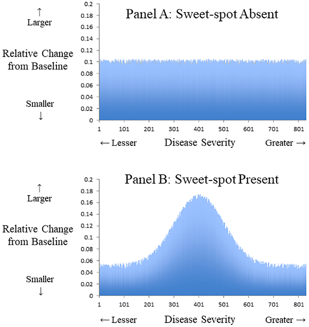
Relative benefit and continuous outcome. Hypothetical data from a trial where primary outcome is a continuous variable that gauges clinical effectiveness. The x-axis denotes disease severity measured at baseline. The y-axis denotes relative change from baseline following treatment. (A) Uniform relative benefit at all levels of disease severity. (B) Potential sweet spot with greater relative benefit at middle range and less benefit at extremes of disease severity. An example could be a diet intervention for overweight patients where the average participant drops 0.1 pounds per day, yet those at extremes of baseline weight have smaller relative changes.

Many patient outcomes are binary indicators rather than continuous variables. In this case, cumulative plots of collective benefits can show the results without resorting to smoothing models or subgroup stratification.¹⁹ For example, a uniform relative benefit at all levels of disease severity might appear as a diagonal line rising with a steady slope above the null (Figure 2A). Conversely, a sweet spot might appear as a sigmoidal curve with a trajectory above the null and a midrange of disproportionate gains (Figure 2B). These cumulative plots are not usually tested in medicine due to a lack of matched data (unlike repeated-measures designs) and due to the reduced statistical power of binary data for identifying a sigmoidal pattern (unlike continuous data).²⁰

Figure 2

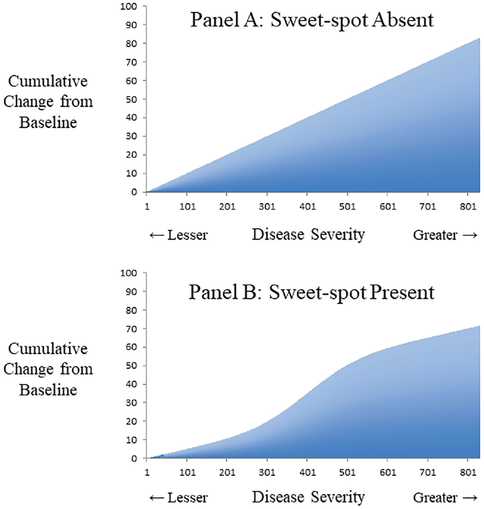
Cumulative benefit and continuous outcome. Hypothetical data from a trial where primary outcome is a continuous variable that gauges clinical effectiveness. The x-axis denotes disease severity measured at baseline. The y-axis denotes cumulative change in outcome from baseline following treatment. (A) Uniform relative benefit at all levels of disease severity. (B) Potential sweet spot with greater relative benefit at middle range and less benefit at extremes of disease severity. An example could be a diet intervention for overweight patients where the total cohort drops 80 pounds per day, yet those at extremes of baseline weight have smaller relative changes.

Testing Sigmoidality

All tests for a sigmoidal pattern face 3 important challenges. First, a linear model might often be a good approximation and leave little remaining systematic variation. Second, sigmoidal functions such as the Gompertz, logistic, or Weibull can be unfamiliar to readers.²¹ Third, a specific sigmoidal function tends to have added degrees of freedom that mandate a check of goodness of fit to avoid overfitting. The net implication is that a sigmoidal function requires large amounts of valid data. This prerequisite may explain why tests for a sigmoidal function are rare in clinical research (despite theorized in common dose–response curves) and tend to be more popular in public health science (such as describing a disease epidemic).

The Gompertz curve is a generalized logistic function developed 2 centuries ago and is the traditional sigmoidal curve for studying numerical growth.^22,23 Similar to all sigmoidal functions, the Gompertz curve describes modest positive beginnings that accelerate in the midrange and decelerate to an upper asymptote. Unlike a conventional logistic function, the Gompertz curve is slightly asymmetric where the upper asymptote is approached more slowly than the initial baseline growth. Diverse applications of the Gompertz curve have included modeling worldwide population counts, forest growth over time, cancer tumor size in laboratory conditions, market uptake of cellular phones, and learning curves from extended education.²⁴

Introducing a Gompertz curve to replace a simple linear model requires checking if the effort is worthwhile. The Akaike information criterion (AIC) was developed half a century ago for model selection based on information theory.²⁵ An AIC can assess different models of the same data to gauge goodness of fit with penalties for adding coefficients (lower values better).²⁶ An AIC can be computed for most statistical models, including linear regression (based on the number of coefficients, residual sum of squares, sample size). An AIC is generally superfluous when checking an individual regression model because each coefficient can be tested directly. The AIC is necessary when evaluating incongruous models such as comparing a linear model to a Gompertz curve.

An additional way to check model validity or avoid overfitting is by cross-validation. Such validation requires splitting the original data into a training sample to derive coefficients and a separate testing sample to examine resulting errors.²⁷ The leave-one-out cross-validation (LOOCV) approach involves computationally intensive techniques that iterate through an entire data set to generate a laborious and unbiased estimate of the error rate.²⁸ The LOOCV approach, therefore, serves to check the superior goodness of fit of a Gompertz model relative to a simple linear model.²⁹ Another strength of this approach is to provide an R² estimate as a more familiar measure of goodness of fit for both the Gompertz model and the linear model.

Clinical Application

In this study, we examined a clinical trial that tested the benefits of an implantable defibrillator for preventing all-cause mortality in cardiac patients.³⁰ By random assignment, one-third received a defibrillator and two-thirds received medical management only. A total of 2,521 patients were followed (median duration = 3.8 years), and overall mortality was lower for the defibrillator group (182 / 829 = 22%) than the control group (484 / 1,692 = 29%), indicating a significant reduction (P < 0.001). Stratification suggested the survival advantage was mostly explained by patients in the middle range of disease severity.³¹ This pattern implies a potential sweet spot in disease severity where some patients experienced more relative benefit than others.

Similar to other clinical trials, this study also collected data on multiple baseline patient features relevant to estimating disease severity. Because no preexisting disease severity index was available, a simple approach was to build a prediction model to determine how these combined baseline features might predict the patient’s outcome over the study duration (see Appendix, available online). This prediction score to gauge disease severity was based solely on the control patients to avoid misinterpreting patients who received a treatment that altered the natural history.³² Such predictive models are also called endogenous stratification in the econometrics literature.³³ Split-sample prevalidation was not included but can be an added way to avoid overfitting disease severity predictions.³⁴

Results

Descriptive Overview

An analysis for identifying a sweet spot requires forming clusters of similar patients.³⁵ In this case, we used a greedy nearest-neighbor matching algorithm (caliper width = 0.2, no replacement) to form triplets where 1 patient received a defibrillator, 2 patients did not receive a defibrillator, and all 3 patients had a similar baseline disease severity score.^36–39 The intent was to convert the randomized trial into a matched randomized trial and estimate an apparent survival advantage for each triplet. Overall, we obtained 829 triplets (sample size = 2,487) that retained all defibrillator patients (n = 829) and most control patients (n = 1,658). The median follow-up was slightly reduced (duration = 3.4 years), and the final outcome counts equaled 661 total deaths.

As expected, these matched patients again showed lower patient mortality in the defibrillator group (182 / 829 = 22%) compared to the control group (479 / 1,658 = 29%), equal to nearly a one-third reduction in odds (odds ratio = 0.69; 95% confidence interval [CI], 0.57–0.84; P < 0.001). The survival advantage with defibrillator treatment was sufficiently clear that it could be confirmed by directly classifying patients as dead or alive at study termination. As in the unmatched analysis, the observed survival advantage was mostly apparent among patients in the middle range of disease severity (Figure 3). Relatively little of the survival advantage from defibrillators was observed for patients with the greatest disease severity or those with the least disease severity.

Figure 3

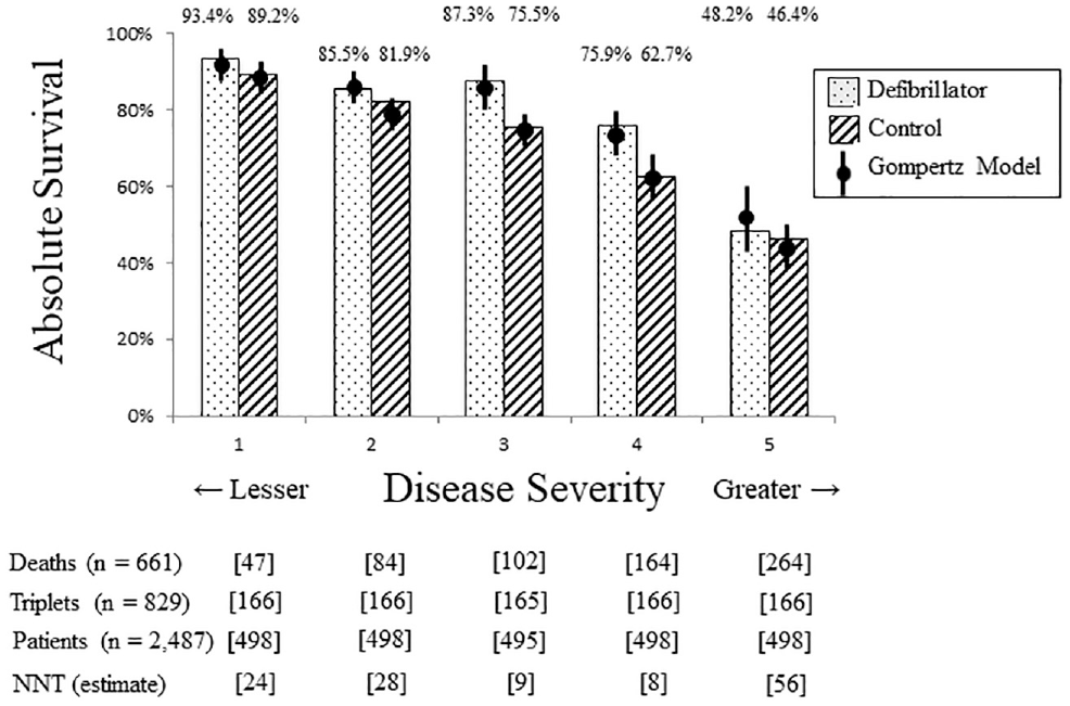
Survival in quintiles of disease severity. Analysis of survival benefit stratified by of five categories of disease severity. X-axis shows disease severity with least severe quintile on left and most severe quintile on right. Y-axis shows proportion of each group alive at study termination. Bars show observed data and circles show results from Gompertz model. Speckled pattern denotes defibrillator group, striped pattern denotes control group, and floating percentages indicate actual survival in each group. Lower square brackets provide count of triplets, individual patients, observed deaths, and estimated number-needed-to-treat (NNT) in each quintile. Results show higher probability of survival with defibrillator treatment for each quintile, accentuated increase in middle quintile, and close fit of Gompertz model with observed data in all quintiles.

The matched cohort then allowed the collective survival advantage to be depicted by a cumulative plot according to the disease severity in each triplet. A triplet where the defibrillator patient survived, 1 control patient died, and the other control survived, for example, suggested a 0.5 patient survival advantage from defibrillator treatment (observed survival = 1.0, expected survival = 0.5). This cumulative plot followed a sigmoidal shape that highlighted how the survival advantage was mostly for patients with midrange severity (Figure 4). The net survival advantage was 57 defibrillator patients (95% CI, 32–80). This latter analysis ignored the timing of death and could be subjected to a global test of statistical significance as a sigmoidal model.

Figure 4

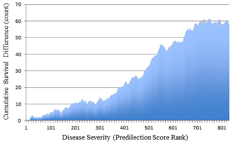
Cumulative survival advantage for defibrillator patients. Histogram of cumulative survival advantage comparing defibrillator patients to control patients. The x-axis shows consecutive triplets of matched patients who are sequenced ordinally by increasing disease severity. The y-axis shows cumulative count of survival advantage for defibrillator patients. Display contains 829 bars for 829 matched triplets (1 defibrillator patient and 2 control patients in each triplet, all with similar disease severity). Results show survival advantage of defibrillator patients mostly explained by individuals with intermediate disease severity.

Linear and Gompertz Models

We analyzed the cumulative survival advantage as a linear model and as a Gompertz model.⁴⁰ The linear model yielded a significant survival advantage across the spectrum of increasing disease severity (intercept = −7.32, β = 0.0847, P < 0.001). As expected, the linear model had high goodness of fit (R² = 95%) and information (AIC = 2,491). Similarly, a Gompertz model yielded a significant survival advantage across the spectrum of increasing disease severity (α = 93, β = 4.939, γ = 0.00316, P < 0.001 for all). As expected, the Gompertz model had high goodness of fit (F = 44,834) and information (AIC = 1,660). The contrast suggested lost information in the linear model compared to the Gompertz model (2,491 v. 1,660, P < 0.001).

The LOOCV approach also confirmed the superior goodness of fit of the Gompertz model (Figure 4).⁴¹ The simple linear model had a median absolute error of 0.068 when comparing observed values to predicted values. The Gompertz model had a median absolute error of 0.029 when checking observed values to predicted values. Overall, this equated to the simple linear model demonstrating a strong relationship of disease severity with accumulating survival advantage (R² = 95.31%) and the Gompertz model demonstrating an even stronger relationship (R² = 99.20%). Model validation through the LOOCV approach indicated this superior goodness of fit was unlikely due to change (P < 0.001).

Alternative Sigmoidal Models

Three alternative sigmoidal models were also considered for sensitivity analysis.²⁴ A logistic model suggested a sweet spot in the midrange of disease severity (α = 115, β = −2.24, ED-50 = 736, P < 0.001 for all) and reasonable information (AIC = 1,823). A Weibull growth model suggested a sweet spot in the midrange of disease severity (α = 74.1, β = 2.28, ED-50 = 617, P < 0.001 for all) and reasonable information (AIC = 1,753). A Chapman–Richards model suggested a sweet spot in the midrange of disease severity (α = 118, β = 0.0019, γ = 2.60, P < 0.001 for all) and reasonable information (AIC = 1,868). Together, the similarity of AIC values confirmed the overall findings of the Gompertz sigmoidal curve.

Extension to Time-to-Event Data

The clinical trial provided a secondary analysis of an alternate end point since outcomes were recorded as time-to-event data (survival analysis) rather than end-of-trial vital status (logistic analysis). This meant 2 patients who both died could have different implications if 1 patient had died later than the other. Addressing this nuance and accounting for censoring required scoring each matched triplet by comparative survival (Appendix). For example, if the defibrillator patient died later than the matched control, the defibrillator patient was scored as superior survival. Other patterns were scored depending on which and when matched patients died (Appendix). This analysis thereby accounted for the timing of death and again yielded a sigmoidal curve to identify a sweet spot (Appendix).

The LOOCV approach also confirmed the superior goodness of fit of the Gompertz model for the time-to-event data. The simple linear model had a median absolute error of 0.049 when checking observed values to predicted values. The Gompertz model had a median absolute error of 0.019 when checking observed values to predicted values. Overall, this equated to the simple linear model demonstrating a strong relationship of disease severity with accumulating survival advantage (R² = 96.96%) and the Gompertz model demonstrating an even stronger relationship (R² = 99.26%). Model validation through the LOOCV approach indicated this superior goodness of fit was unlikely due to change (P < 0.001).

Model Interpretation

The coefficients from a Gompertz curve can be difficult to interpret. As one approach, we modeled the estimated survival advantage for each quintile of disease severity (Figure 3). We found a substantial reduction in mortality for patients in the mid-zone of disease severity (estimated odds ratio = 0.52; 95% CI, 0.32–0.86). In contrast, we found modest reductions in mortality for patients with the lowest severity (estimated odds ratio = 0.68; 95% CI, 0.35–1.33) or highest severity (estimated odds ratio = 0.71; 95% CI, 0.49–1.02). For example, the highest-severity patients showed relatively modest absolute survival gains with a defibrillator, equal to a number needed to treat of 56 to avoid 1 death.

A different approach to interpreting Gompertz models is based on the coefficients. A linear model, for example, presumes a consistent marginal benefit regardless of severity with a slope that estimates the gains for an average triplet. In our case, a slope of 0.0847 means treatment for the average triplet saves 0.0847 lives, implying a number needed to treat of 12 to avoid 1 death (1 / 0.0847). Similarly, the inflection point of a Gompertz curve yields a slope calculated from the amplitude and curvature (slope = α×γ / e) that estimates the gains at the sweet spot. In our case, a slope of 0.1081 (93 × 0.00316 / 2.7183) means treatment for the sweet-spot triplet saves 0.1081 lives, implying a number needed to treat of 9 to avoid 1 death (1 / 0.1081).

Discussion

In this article, we focus on the concept of a sweet spot in a randomized trial and introduce a method testing whether a study might underestimate or overestimate the effects of a treatment on diverse patients. The core assumption is that a sweet spot is related to disease severity. The strategy is to explore for a sigmoidal relationship of disease severity with cumulative treatment effect (Box). The analysis then tests whether a sigmoidal relationship is superior to a linear relationship for describing accumulating differences. In follow-up to prior theory, the approach does not rely on subgroup stratification.⁴² Using this method, we detected a potential sweet spot in a randomized trial of defibrillators for preventing mortality in cardiac patients.

Box

Identifying a Sweet Spot in a Randomized Trial^a

General Steps for a Sweet-Spot Analysis

• Build a severity score based on controls

• Compute each patient’s baseline severity

• Assemble matched clusters with similar severity

• Determine the apparent benefit in each cluster

• Assess cumulative benefit with increasing severity

• Inspect for an apparent sigmoid shape

• Test sigmoid model against linear model

• Show results translated back to natural units

General Limitations of a Sweet-Spot Analysis

• Spurious P values from capitalizing on chance

• Insufficient sample size and diversity

• Fallible estimations of disease severity

• Faulty matching algorithm

• Mistaken selection of a particular sigmoidal model

• Inability to estimate exact boundary of sweet spot

• Trivial clinical magnitude of estimated sweet spot

• Propagation of failures in underlying trial design

• Vulnerability to data falsification

• Difficulties generalizing to other patient populations

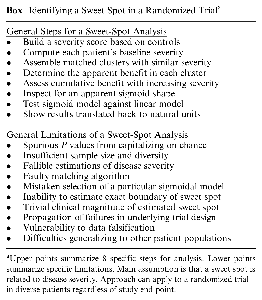
Upper points summarize 8 specific steps for analysis. Lower points summarize specific limitations. Main assumption is that a sweet spot is related to disease severity. Approach can apply to a randomized trial in diverse patients regardless of study end point.

Our method has limitations. The creation of matched sets requires extending the concept of a randomized trial to imply patients tend to be balanced both at the sample average and at finer substratifications. The functional form of a sigmoidal curve differs from polynomial or spline regressions that provide more complex models for studying nonlinear associations.⁴³ The actual coefficients of a sigmoidal curve of cumulative benefit can also vary slightly depending on whether later matched sets are scaled in a weighted or unweighted manner. The subsequent estimates for pinpointing a sweet spot are imprecise and do not identify exact boundaries for a sweet spot. The analyses do not directly account for equity, diversity, inclusion, or other societal priorities.

Several other methods are available as alternative ways of testing how treatment effects might vary by patient characteristics. Forest plots can provide separate analyses based on individual characteristics but can also create type I or type II statistical errors, unlike a single test based on a severity score. Regression analysis with interaction terms is an approach in population epidemiology that can also be hard for clinicians to interpret, unlike a visual display that can show relative risk, absolute risk, or number needed to treat. More advanced generalized estimating equations can allow other functional forms but tend to also require substantial sophistication and iteration, unlike our approach that can be standardized.

Testing for a sweet spot in a clinical trial is rarely the primary analysis (unless testing a treatment known to be effective or theorized to have a highly responsive subgroup). As such, a sweet-spot analysis deserves skepticism due to the risk of multiple hypothesis testing and capitalizing on chance. The study sample needs to have substantial variability in disease severity that can be quantified in a single metric.⁴⁴ A matching algorithm must also be available to assemble clusters of matched patients randomized to different treatments.^45–47 Overall, a study will require plentiful sample size and outcome events to avoid overfitting.⁴⁸ The importance of these conditions may explain why a sweet-spot analysis of randomized trials is often discussed but rarely attempted.³

A related caveat is the risk of a false-negative analysis and mistakenly concluding no sweet spot is present. Indeed, it is impossible to prove a sweet spot does not exist. The specific trial analyzed herein suggests the relative benefit of a defibrillator in reducing mortality depends on disease severity. The same pattern might also help explain why a subsequent trial of patients who had mild disease severity found no significant mortality benefit.⁴⁹ Together, the modest results might have undercut enthusiasm for an effective intervention and indirectly promoted costly alternatives such as external defibrillators in public spaces.^50–52 More generally, the basic concept of a sweet spot could help inform cost-effectiveness analyses and policy decisions around expensive interventions.

Future research can extend ideas in different directions. Methodologists could address different severity scores and different sigmoidal functional forms. Experts in machine learning could develop high-dimensional algorithms for creating matched sets of similar patients.⁵³ Statisticians might also wish to tackle more complex cases that include competing risks or when a sweet spot is not unimodal. Policy analysts could conduct simulations to assess how differences in patient recruitment might shift subsequent study results. Meta-analysts could consider how to incorporate a sweet spot into the GRADE framework.⁵⁴ Trialists could adopt our approach to review the frequency of a sweet spot in past randomized trials in diverse fields. We encourage these and other directions for future research.

Public domain software for an R module is now in development for the CRAN site to help guard against faulty execution and other statistical nuances of a sweet-spot analysis. Of course, no analysis can compensate for a failure of randomization, lack of blinding, specious second-guessing, or other biases in study design.⁵⁵ In addition, scientists are prone to self-deception that can be exacerbated by sunk-cost reasoning in the aftermath of a costly trial.⁵⁶ A small amount of data falsification, furthermore, can quickly cause spurious results when estimating a sigmoidal function. These caveats merit attention since the methodology described here can be readily replicated in randomized trials worldwide to check whether a potential sweet spot might be important.

Supplemental Material

sj-pdf-1-mdm-10.1177_0272989X211025525 – Supplemental material for Testing for a Sweet Spot in Randomized Trials

Supplemental material, sj-pdf-1-mdm-10.1177_0272989X211025525 for Testing for a Sweet Spot in Randomized Trials by Donald A. Redelmeier, Deva Thiruchelvam and Robert J. Tibshirani in Medical Decision Making

Footnotes

Acknowledgements

We thank Peter Austin, Erin Craig, Michael Fralick, Fizza Manzoor, Cindy Mian-Mian, Sheharyar Raza, Therese Stukel, Jonathan Zipursky, and the Stanford biostatistics group for helpful suggestions on specific points.

The author(s) declared no potential conflicts of interest with respect to the research, authorship, and/or publication of this article.

The author(s) disclosed receipt of the following financial support for the research, authorship, and/or publication of this article: This project was supported by a Canada Research Chair in Medical Decision Sciences, the Canadian Institutes of Health Research, and the BrightFocus Foundation. The views expressed are those of the authors and do not necessarily reflect the Ontario Ministry of Health & Long-term Care.

Data Sharing

The deidentified data collected for this study are available in an appendix included at the time of original manuscript submission and also are available following publication for researchers whose proposed use of data has been approved by an independent review committee.

ORCID iD

Donald A. Redelmeier

Supplemental Material

Supplementary material for this article is available on the Medical Decision Making website at .

References

Pitt

Zannad

Remme

, et al. Effect of spironolactone on morbidity and mortality in patients with heart failure. Randomized Aldactone Evaluation Study Investigators. N Engl J Med. 1999;341(10):709–17.

Caverly

Prochazka

Binswanger

Kutner

Matlock

. Confusing relative risk with absolute risk is associated with more enthusiastic beliefs about the value of cancer screening. Med Decis Making. 2014;34(5):686–92.

Kent

Paulus

van Klaveren

, et al. The predictive approaches to treatment effect heterogeneity (PATH) statement. Ann Intern Med. 2020;172(1):35–45.

Caverly

Prochazka

Combs

, et al. Doctors and numbers: an assessment of the critical risk interpretation test. Med Decis Making. 2015;35(4):512–24.

Heath

Manolopoulou

Baio

. A review of methods for analysis of the expected value of information. Med Decis Making. 2017;37(7):747–58.

Tolbert

Brundage

Bantug

, et al. Picture this: presenting longitudinal patient-reported outcome research study results to patients. Med Decis Making. 2018;38(8):994–1005.

Alper

. Searching for medicine’s sweet spot. Science. 2001;291(5512):2338–43.

Hulley

Cummings

Browner

Grady

Newman

. Designing Clinical Research. Philadelphia, PA: Lippincott Williams & Wilkins; 2013.

Blanke

DeMatteo

. Duration of adjuvant therapy for patients with gastrointestinal stromal tumors: where is goldilocks when we need her? JAMA Oncol. 2016;2(6):721–2.

10.

Jhun

Wei

Herbert

. The neonatal airway and the Goldilocks phenomenon. Ann Emerg Med. 2017;69(2):167–70.

11.

Kent

Nelson

Dahabreh

Rothwell

Altman

Hayward

. Risk and treatment effect heterogeneity: re-analysis of individual participant data from 32 large clinical trials. Int J Epidemiol. 2016;45(6):2075–88.

12.

Watson

Holmes

. Graphing and reporting heterogeneous treatment effects through reference classes. Trials. 2020;21(1):386.

13.

Redelmeier

Tibshiran

. An approach to explore for a sweet spot in randomized trials. J Clin Epidemiol. 2020;120:59–66.

14.

Basu

Carlson

Veenstra

. A framework for prioritizing research investments in precision medicine. Med Decis Making. 2016;36(5):567–80.

15.

Austin

. An introduction to propensity score methods for reducing the effects of confounding in observational studies. Multivariate Behav Res. 2011;46(3):399–424.

16.

Wicherts

Veldkamp

Augusteijn

Bakker

van Aert

van Assen

. Degrees of freedom in planning, running, analyzing, and reporting psychological studies: a checklist to avoid p-hacking. Front Psychol. 2016;7:1832.

17.

Gillespie

. Understanding waterfall plots. J Adv Pract Oncol. 2012;3(2):106–11.

18.

Kwak

Bang

Camidge

, et al. Anaplastic lymphoma kinase inhibition in non-small-cell lung cancer. N Engl J Med. 2010;363(18):1693–703.

19.

Larson

. Descriptive statistics and graphical displays. Circulation. 2006;114(1):76–81.

20.

Moses

. Graphical methods in statistical analysis. Annu Rev Public Health. 1987;8:309–53.

21.

Yin

Goudriaan

Lantinga

Vos

Spiertz

. A flexible sigmoid function of determinate growth. Ann Bot. 2003;91(3):361–71.

22.

Gompertz

. On the nature of the function expressive of the law of human mortality, and on a new mode of determining the value of life contingencies. Phil Trans R Soc B Biol Sci. 1825;182:513–85.

23.

Makeham

. On the integral of Gompertz’s function for expressing the values of sums depending upon the contingency of life. J Instit Actuaries. 1873;17(5):305–27.

24.

Tjørve

KMC

Tjørve

. The use of Gompertz models in growth analyses, and new Gompertz-model approach: an addition to the Unified-Richards family. PLoS One. 2017;12(6):e0178691.

25.

Akaike

. A new look at the statistical model identification. IEEE Trans Autom Control. 1974;19:716–23.

26.

Vrieze

. Model selection and psychological theory: a discussion of the differences between the Akaike information criterion (AIC) and the Bayesian information criterion (BIC). Psychol Methods. 2012;17(2):228–43.

27.

Lachenbruch

Mickey

. Estimation of error rates in discriminant analysis. Technometrics. 1968;10(1):1–11.

28.

James

Witten

Hastie

Tibshirani

. An Introduction to Statistical Learning. New York: Springer; 2013.

29.

Friedman

Hastie

Tibshirani

. The Elements of Statistical Learning. New York: Springer; 2001.

30.

Bardy

Lee

Mark

, et al., for the Sudden Cardiac Death in Heart Failure Trial (SCD-HeFT) Investigators. Amiodarone or an implantable cardioverter-defibrillator for congestive heart failure. N Engl J Med. 2005;352(3):225–37.

31.

Redelmeier

Tibshiran

. An approach to explore for a sweet spot in randomized trials. J Clin Epidemiol. 2020;120:59–66.

32.

Sackett

Haynes

Tugwell

. Clinical Epidemiology: A Basic Science for Clinical Medicine. Boston: Little, Brown; 1985.

33.

Abadie

Chingos

West

. Endogenous stratification in randomized experiments. Rev Econ Stat. 2018;100(4):567–80.

34.

Höfling

Tibshirani

. A study of pre-validation. Ann Appl Stat. 2008;2(2):643–64.

35.

Rosenbaum

Rubin

. Constructing a control group using multivariate matched sampling methods that incorporate the propensity score. Am Stat. 1985;39(1):33–8.

36.

Parsons

. Reducing bias in a propensity score matched-pair sample using greedy matching. Available from: https://www.researchgate.net/publication/253998470_Reducing_Bias_in_a_Propensity_Score_Matched-Pair_Sample_Using_Greedy_Matching_Techniques

37.

Austin

. Statistical criteria for selecting the optimal number of untreated subjects matched to each treated subject when using many-to-one matching on the propensity score. Am J Epidemiol. 2010;172(9):1092–7.

38.

Austin

. Optimal caliper widths for propensity-score matching when estimating differences in means and differences in proportions in observational studies. Pharm Stat. 2011;10(2):150–61.

39.

Austin

. A comparison of 12 algorithms for matching on the propensity score. Stat Med. 2014;33(6):1057–69.

40.

Seber

Wild

. Nonlinear Regression. New York: John Wiley; 1989.

41.

Molinaro

Simon

Pfeiffer

. Prediction error estimation: a comparison of resampling methods. Bioinformatics. 2005;21(15):3301–7.

42.

Redelmeier

Tibshiran

. An approach to explore for a sweet spot in randomized trials. J Clin Epidemiol. 2020;120:59–66.

43.

Heinzl

Kaider

. Gaining more flexibility in Cox proportional hazards regression models with cubic spline functions. Comput Methods Programs Biomed. 1997;54(3):201–8.

44.

Burke

Hayward

Nelson

Kent

. Using internally developed risk models to assess heterogeneity in treatment effects in clinical trials. Circ Cardiovasc Qual Outcomes. 2014;7(1):163–9.

45.

D’Agostino

Jr.

Propensity score methods for bias reduction in the comparison of a treatment to a non-randomized control group. Stat Med. 1998;17(19):2265–81.

46.

Dehejia

Wahba

. Propensity score-matching methods for nonexperimental causal studies. Rev Econ Stat. 2002;84(1):151–61.

47.

Austin

Stuart

. Estimating the effect of treatment on binary outcomes using full matching on the propensity score. Stat Methods Med Res. 2017;26(6):2505–25.

48.

van Klaveren

Balan

Steyerberg

Kent

. Models with interactions overestimated heterogeneity of treatment effects and were prone to treatment mistargeting. J Clin Epidemiol. 2019;114:72–83.

49.

Køber

Thune

Nielsen

, et al.; DANISH Investigators. Defibrillator implantation in patients with nonischemic systolic heart failure. N Engl J Med. 2016;375(13):1221–30.

50.

Groeneveld

Kwong

Liu

, et al. Cost-effectiveness of automated external defibrillators on airlines. JAMA. 2001;286(12):1482–9.

51.

Bailey

Hodges

Church

. Decision to implant a cardioverter defibrillator after myocardial infarction: the role of ejection fraction v. other risk factor markers. Med Decis Making. 2007;27(2):151–60.

52.

Andersen

Holmberg

Granfeldt

James

Caulley

. Cost-effectiveness of public automated external defibrillators. Resuscitation. 2019;138:250–8.

53.

Stuart

. Matching methods for causal inference: a review and a look forward. Stat Sci. 2010;25(1):1–21.

54.

Guyatt

Oxman

Vist

, et al. GRADE: an emerging consensus on rating quality of evidence and strength of recommendations. BMJ. 2008;336(7650):924–6.

55.

Alshreef

Latimer

Tappenden

, et al. Statistical methods for adjusting estimates of treatment effectiveness for patient nonadherence in the context of time-to-event outcomes and health technology assessment: a systematic review of methodological papers. Med Decis Making. 2019;39(8):910–25.

56.

Kwon

Allen

Scherer

, et al. The effect of total cost information on consumer treatment decisions: an experimental survey. Med Decis Making. 2018;38(5):584–92.

Supplementary Material

Please find the following supplemental material available below.

For Open Access articles published under a Creative Commons License, all supplemental material carries the same license as the article it is associated with.

For non-Open Access articles published, all supplemental material carries a non-exclusive license, and permission requests for re-use of supplemental material or any part of supplemental material shall be sent directly to the copyright owner as specified in the copyright notice associated with the article.

0.00 MB

0.53 MB