Sage Journals: Discover world-class research

Abstract

In meta-analysis, between-study heterogeneity indicates the presence of effect-modifiers and has implications for the interpretation of results in cost-effectiveness analysis and decision making. A distinction is usually made between true variability in treatment effects due to variation in patient populations or settings and biases related to the way in which trials were conducted. Variability in relative treatment effects threatens the external validity of trial evidence and limits the ability to generalize from the results; imperfections in trial conduct represent threats to internal validity. We provide guidance on methods for meta-regression and bias-adjustment, in pairwise and network meta-analysis (including indirect comparisons), using illustrative examples. We argue that the predictive distribution of a treatment effect in a “new” trial may, in many cases, be more relevant to decision making than the distribution of the mean effect. Investigators should consider the relative contribution of true variability and random variation due to biases when considering their response to heterogeneity. In network meta-analyses, various types of meta-regression models are possible when trial-level effect-modifying covariates are present or suspected. We argue that a model with a single interaction term is the one most likely to be useful in a decision-making context. Illustrative examples of Bayesian meta-regression against a continuous covariate and meta-regression against “baseline” risk are provided. Annotated WinBUGS code is set out in an appendix.

Keywords

cost-effectiveness analysis Bayesian meta-analysis comparative effectiveness systematic reviews

When combining results of different studies in a meta-analysis, heterogeneity (i.e., between-trials variation in relative treatment effects) has implications for the interpretation of results and decision making. We provide guidance on techniques that can be used to explore the reasons for heterogeneity, as recommended in the National Institute for Health and Clinical Excellence (NICE) Guide to Methods of Technology Appraisal.¹ We focus particularly on the implications of different forms of heterogeneity, the technical specification of models that can estimate or adjust for potential causes of heterogeneity, and the interpretation of such models in a decision-making context. There is a considerable literature on the origins and measurements of heterogeneity,² and this is beyond the scope of this article.

Heterogeneity in treatment effects is an indication of the presence of effect-modifying mechanisms—in other words, of interactions—between the treatment effect and the trial or trial-level variable. A distinction is usually made between 2 kinds of interaction effects: clinical variation in treatment effects, resulting from variation between treatment effects due to different patient populations, settings, or protocols across trials and deficiencies in the way the trial was conducted. The first type of interaction is said to represent a threat to the external validity of trials, limiting the extent to which one can generalize trial results from one situation to another. The second threatens the internal validity of trials: the trial delivers a biased estimate of the treatment effect in its target population, which may or may not be the same as the target population for decision. Typically, these biases are considered to vary randomly over trials and do not necessarily have a zero mean. For example, the biases associated with markers of poor trial quality, such as lack of allocation concealment or lack of double blinding, have been shown to be associated with larger treatment effects.^3,4 A general model for heterogeneity that encompasses both types of interaction has been proposed,⁵ but it is seldom possible to determine what the causes of heterogeneity are and how much is due to true variation in clinical factors and how much is due to other unknown causes of biases.

In a decision-making context, the response to high levels of heterogeneity is a critical issue. Investigators should compare the size of the treatment effect with the extent of between-trials variation. If the latter approximates the former, interpretation of mean treatment effects is difficult.^6,7 Figure 1 portrays a situation in which a random effects (RE) model has been fitted. The posterior mean of the mean treatment effect is 0.70 with a posterior standard deviation (SD) of 0.2, making the mean effect clearly different from zero with a 95% credible interval (CrI) of (0.31, 1.09). However, the posterior mean of the between-trials standard deviation is σ = 0.68, comparable in size to the mean effect. What is a reasonable confidence interval for our prediction of the outcome of a future trial of infinite size? An approximate answer in classical statistics is found by adding the variance of the mean to the between-trials variance, which gives SD²+σ² = 0.50, giving a predictive standard deviation of 0.71. Note that the 95% predictive interval is now (−0.69, 2.09), easily spanning zero effect, including a range of harmful effects. If we interpret these distributions in a Bayesian way, we would find that the probability that the mean effect is less than zero is only 0.0002, whereas the probability that a new trial would show a negative effect is much higher: 0.162 (Figure 1).

Figure 1

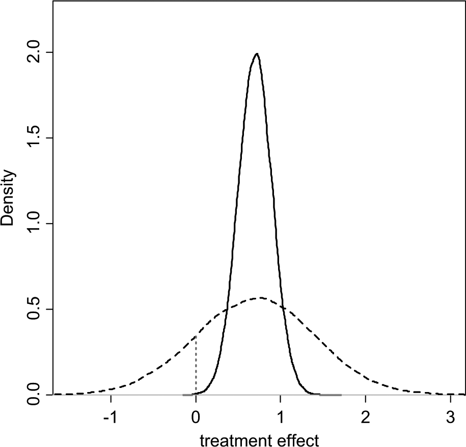
Posterior (solid) and predictive (dashed) densities for a treatment effect with mean = 0.7, standard deviation = 0.2, and heterogeneity (standard deviation) = 0.68. The area under the curve to the left of the vertical dotted line is the probability of a negative value for the treatment effect.

This issue has been discussed before,^{5

–8} and it has been proposed that, in the presence of heterogeneity, the predictive distribution, rather than the distribution of the mean treatment effect, better represents our uncertainty about the comparative effectiveness of treatments in a future “rollout” of a particular intervention. In a Bayesian Markov chain Monte Carlo (MCMC) setting, a predictive distribution is easily obtained by drawing further samples from the distribution of effects:

δ_{new} ~ N (d, σ^{2}),

where d is the estimated (common) mean treatment effect and σ² the estimated between-trial heterogeneity variance.

Where there are high levels of unexplained heterogeneity, the implications of this recommendation for the uncertainty in a decision can be quite profound, and it is therefore important that the degree of heterogeneity is not exaggerated and that the causes of the heterogeneity are investigated.^9,10 The variance term in the predictive distribution should consist only of true variation between trial populations,⁵ but at present, there is no clear methodology to distinguish between different sources of variation in treatment effect. Recent meta-epidemiological work on the determinants of between-study variation is beginning to shed some light on this.¹¹

Meta-regression is used to relate the size of a treatment effect obtained from a meta-analysis to potential effect modifiers—covariates—that may be characteristics of the trial participants or connected with the trial setting or conduct. These covariates may be categorical or continuous. In common with other forms of meta-analysis, meta-regression can be based on aggregate (trial-level) outcomes and covariates, or individual patient data (IPD) and covariates when available. However, even if we restrict attention to randomized controlled trial (RCT) data, the study of effect-modifiers is inherently observational^2,12 as it is not possible to randomize patients to one covariate value or another. As a consequence, meta-regression inherits all the difficulties of interpretation and inference that attach to nonrandomized studies: confounding, correlation between covariates, and, most important, the inability to infer causality from association.

We provide guidance on methods for meta-regression and bias-adjustment that can address the presence of heterogeneity using aggregate data and trial-level covariates and discuss the limitations of this approach and the potential advantages of meta-regression with IPD.

Subgroup Effects (Appendix: Example 1)

We start with the simplest form of meta-regression: adjusting for subgroup effects in a pairwise meta-analysis. The theory set out in this section is then generalized to other types of meta-regression and to multiple treatments. The methods outlined here can be seen as extensions to the common generalized linear modeling framework for pairwise and network meta-analysis.¹³

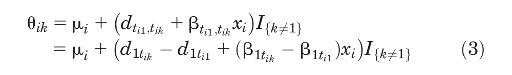
In the context of treatment effects in RCTs, a subgroup effect can be understood as a categorical trial-level covariate that interacts with the treatment. The hypothesis would be that the size of the treatment effect is different, for example, in male and female patients or that it depends on age group or previous treatment. Separate analyses can be carried out for each group and the relative treatment effects compared. However, if the models have random treatment effects, having separate analyses means having different estimates of between-trial variation. As there are seldom enough data to estimate the between-trial variation, it may make more sense to assume that it is the same for all subgroups. Furthermore, running separate analyses does not immediately produce the test of interaction that is required to reject the null hypothesis of equal effects. It is therefore preferable to have a single integrated analysis with a single between-trial variation term and an interaction term, β, introduced on the treatment effect, as follows:

θ_{ik} = μ_{i} + (δ_{i, 1 k} + β x_{i}) I_{{k \neq 1}},

(1)

where x_i is the trial-level covariate for trial i, which can represent a subgroup, a continuous covariate, or baseline risk; θ_ik is the linear predictor¹³ (e.g., the log-odds or mean) in arm k of trial i;µ_i are the trial-specific baseline effects in a trial i, treated as unrelated nuisance parameters; δ_i,1k are the trial-specific treatment effects of the treatment in arm k relative to the treatment in arm 1 in that trial, with k = 1, 2 and

I_{{u}} = {\begin{matrix} 1 & if u is true \\ 0 & otherwise \end{matrix}

(2)

We can rewrite equation (1) as

\begin{matrix} θ_{i 1} = μ_{i} \\ θ_{i 2} = μ_{i} + δ_{i, 12} + β x_{i} \end{matrix}

and note that the treatment and covariate interaction effects (δ and β) act only in the experimental arm, not in the control. For an RE model, the trial-specific log-odds ratios come from a common distribution: $δ_{i, 12} ~ N (d_{12}, σ^{2})$ . For a fixed effect (FE) model, we replace equation (1) with $θ_{ik} = μ_{i} + (d_{12} + β x_{i}) I_{{k \neq 1}}$ . In the Bayesian framework d ₁₂, β and σ will be given independent (noninformative) priors: for example, d ₁₂, β ~ N(0, 100²) and σ ~ Uniform(0, 5).

Meta-Regression Models in Network Meta-Analysis

In a network meta-analysis (NMA) context, variability in relative treatment effects can also induce inconsistency¹⁴ across pairwise comparisons. The methods introduced here are therefore also appropriate for dealing with inconsistency. Unless otherwise stated, when we refer to heterogeneity in this context, this can be interpreted as heterogeneity and/or inconsistency.

A large number of meta-regression models can be proposed for NMA, each with very different implications. There are 3 main approaches: unrelated interaction terms for each treatment, exchangeable and related interaction terms, and one single interaction effect for all treatments. We argue that the third model is the most likely to have a useful interpretation in a decision-making context.

Consider a binary between-trial covariate (e.g., primary v. secondary prevention trials) in a case where s treatments are being compared.^15,16 We take treatment 1 (e.g., a placebo or standard treatment) as the reference treatment in the NMA. Following the approach to consistency models adopted previously,¹³ we have (s– 1) basic parameters for the relative treatment effects d ₁₂, d ₁₃, . . ., d _1s of each treatment relative to treatment 1. The remaining (s– 1)(s– 2)/2 treatment contrasts are expressed in terms of these parameters using the consistency equations: for example, the effect of treatment 4 compared with treatment 3 is written as d ₃₄ = d ₁₄–d ₁₃.¹³ We set out a range of fixed treatment effect interaction models, which are later extended to random treatment effects.

1. Unrelated Treatment-Specific Interactions

If there is an interaction effect between, say, primary/secondary prevention and treatment, but these interactions are different for every treatment, the model will have as many interaction terms as there are basic treatment effects (e.g., β₁₂, β₁₃, . . ., β_1s), each representing the additional (interaction) treatment effect in secondary prevention (compared with primary) in comparisons of treatments 2, 3, . . ., s to treatment 1. These terms are exactly parallel to the main effects d ₁₂, d ₁₃, . . ., d _1s, which now represent the treatment effects in primary prevention populations. As with the main effects, for trials comparing, say, treatments 3 and 4, the interaction term is the difference between the interaction terms on the effects relative to treatment 1, so that β₃₄ = β₁₄–β₁₃. The fixed treatment effects model for the linear predictor is

\begin{matrix} θ_{ik} = μ_{i} + (d_{t_{i 1}, t_{ik}} + β_{t_{i 1}, t_{ik}} x_{i}) I_{{k \neq 1}} \\ = μ_{i} + (d_{1 t_{ik}} - d_{1 t_{i 1}} + (β_{1 t_{ik}} - β_{1 t_{i 1}}) x_{i}) I_{{k \neq 1}} \end{matrix}

(3)

with t_ik representing the treatment in arm k of trial i, x_i the covariate/subgroup indicator, and I defined in equation (2). In all models, we set d ₁₁ = β₁₁ = 0. The remaining interaction terms are given unrelated vague prior distributions in a Bayesian analysis.

The relative treatment effects in secondary prevention are d ₁₂+β₁₂, d ₁₃+β₁₃, . . ., d _1s+β_1s. The interpretation is that the relative efficacy of each of the s treatments in primary prevention populations is entirely unrelated to their relative efficacy in secondary prevention populations.

2. Exchangeable and Related Treatment-Specific Interactions

This model has the same structure as the model above, but now the (s– 1) “basic” interaction terms are drawn from a random distribution with a common mean and between-treatment variance: $β_{1 k} ~ N (b, τ^{2})$ , for treatment k = 2, . . ., s. The mean interaction effect and its variance are estimated from the data, although informative priors that limit how similar or different the interaction terms are can be used. The interpretation is that there are real differences between the relative treatment effects, although these are centered on a common mean, with a common variance.

3. Same Interaction Effect for All Treatments

In this case, there is a single interaction term b that applies to the relative effects of all the treatments relative to treatment 1, so that $β_{1 k} = b$ for k = 2, . . ., s. The treatment effects relative to treatment 1, d₁₂, d ₁₃…d _1s in primary prevention, are all higher or lower by the same amount, b in secondary prevention: d ₁₂+b, d ₁₃+b . . . d _1s+b. However, the effects of treatments 2, 3, . . ., s relative to each other in primary and secondary prevention populations are the same because the interaction terms cancel out. For example, consider the effect of treatment 4 relative to treatment 3 in secondary prevention: $d_{14} + b - (d_{13} + b) = d_{14} - d_{13}$ , which is the same as in primary prevention. This means that the choice of reference treatment becomes important, and results for models with covariates are sensitive to this choice.

Note that although we have presented the models in the context of subgroup effects, models for meta-regression with continuous covariates, including baseline risk, have the same structure.

If an unrelated interactions model is being considered (model 1), this requires 2 connected networks (one for each subgroup), including all the treatments, that is, with at least (s– 1) trials in each. With related interaction effects (model 2), it may not be necessary to have 2 complete networks, but a substantial number of trials are needed to identify both random treatment effects and random interactions. However, to use such a model, there needs to be a clear rationale for exchangeability of interactions with a common mean and variance. One rationale could be to allow for different covariate effects for different treatments within the same class. Thus, treatment 1 is a standard or placebo treatment, whereas some of the treatments 2, . . ., s belong to a “class.” For example, one might imagine one set of exchangeable interaction terms for aspirin-based treatments for atrial fibrillation relative to placebo and a second set of interactions for warfarin-based treatments relative to placebo.¹⁷

Although exchangeable and related interactions seem an attractive model in theory, they could lead to situations where the relative efficacy or the relative cost-effectiveness of a set of active treatments in the same class, and hence optimal treatment decisions, will depend on covariate values. However, differences between interaction terms are unlikely to be robust, and treatment decisions could then be driven by statistically insignificant interaction terms. Therefore, although these more complex models can be fitted,^17,18 their best role may be in exploratory analyses. Here we explore only model 3, which assumes an identical interaction effect across all treatments with respect to the reference treatment.

Network Meta-Regression with a Continuous Covariate

When dealing with a continuous covariate, we will use centered covariate values.¹⁹ This is achieved by subtracting the mean covariate value, $\bar{x}$ , from each x_i . To fit a random treatment effects model that assumes a common interaction effect for all treatments with covariate centering, we rewrite equation (3) as

θ_{ik} = μ_{i} + (δ_{i, 1 k} + (β_{1 t_{ik}} - β_{1 t_{i 1}}) (x_{i} - \bar{x})) I_{{k \neq 1}},

(4)

where β₁₁ = 0, β_1k = b (k = 2, . . . ,7) and $δ_{i, 1 k} ~ N (d_{1 t_{ik}} - d_{1 t_{i 1}}, σ^{2})$ .

We retain the treatment-specific interaction effects but set them all equal to b, so that the terms cancel out in comparisons not involving the reference treatment. To produce treatment effect estimates at covariate value z, the outputs from this model should be “uncentered”: $d_{1 k} - b (\bar{x} - z)$ , k = 2, . . ., s.

Example: Certolizumab Meta-Regression on Mean Disease Duration (Appendix: Example 2)

Data are available from a review of trials of certolizumab pegol (CZP) for the treatment of rheumatoid arthritis in patients who had failed on disease-modifying antirheumatic drugs, including methotrexate (MTX).²⁰ Twelve MTX controlled trials were identified, comparing 6 different treatments with placebo (Figure 2).

Figure 2

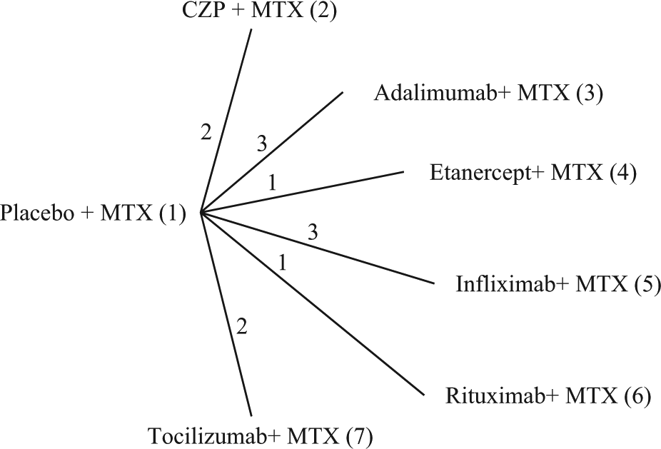
Certolizumab example²⁰: treatment network. Lines connecting 2 treatments indicate that a comparison between these treatments has been made. The numbers on the lines indicate how many randomized controlled trials compare the 2 connected treatments. CZP, certolizumab pegol; MTX, methotrexate.

Table 1 shows the number of patients who have improved by at least 50% on the American College of Rheumatology scale (ACR50) at 6 months, r_ik , out of all included patients, n_ik , for each arm of the included trials, along with the mean disease duration in years for patients in each trial, x_i (i = 1, . . ., 12; k = 1, 2). The crude odds ratios (ORs) from Table 1 are plotted (on a log-scale) against mean disease duration in Figure 3, with the numbers 2 to 7 representing the OR of that treatment relative to placebo plus MTX (chosen as the reference treatment). Example 1 in the Appendix gives details of priors and the WinBUGS²¹ code for the model in equation (4).

Table 1

Certolizumab Example²⁰: Number of Patients Achieving ACR50 at 6 Months,^a r, Out of the Total Number of Patients, n, in Arms 1 and 2 of the 12 Trials and Mean Disease Duration (in Years) for Patients in Trial i, x_i

			Arm 1		Arm 2
Study Name	Treatment in Arm 1, t_i ₁	Treatment in Arm 2, t_i ₂	No. Achieving ACR50, r_i ₁	Total No. of Patients, n_i ₁	No. Achieving ACR50, r_i ₂	Total No. of Patients, n_i ₂	Mean Disease Duration (Years), x_i
RAPID 1	Placebo	CZP	15	199	146	393	6.15
RAPID 2	Placebo	CZP	4	127	80	246	5.85
Kim 2007	Placebo	Adalimumab	9	63	28	65	6.85
DE019	Placebo	Adalimumab	19	200	81	207	10.95
ARMADA	Placebo	Adalimumab	5	62	37	67	11.65
Weinblatt 1999	Placebo	Etanercept	1	30	23	59	13
START	Placebo	Infliximab	33	363	110	360	8.1
ATTEST	Placebo	Infliximab	22	110	61	165	7.85
Abe 2006^b	Placebo	Infliximab	0	47	15	49	8.3
Strand 2006	Placebo	Rituximab	5	40	5	40	11.25
CHARISMA^b	Placebo	Tocilizumab	14	49	26	50	0.915
OPTION	Placebo	Tocilizumab	22	204	90	205	7.65

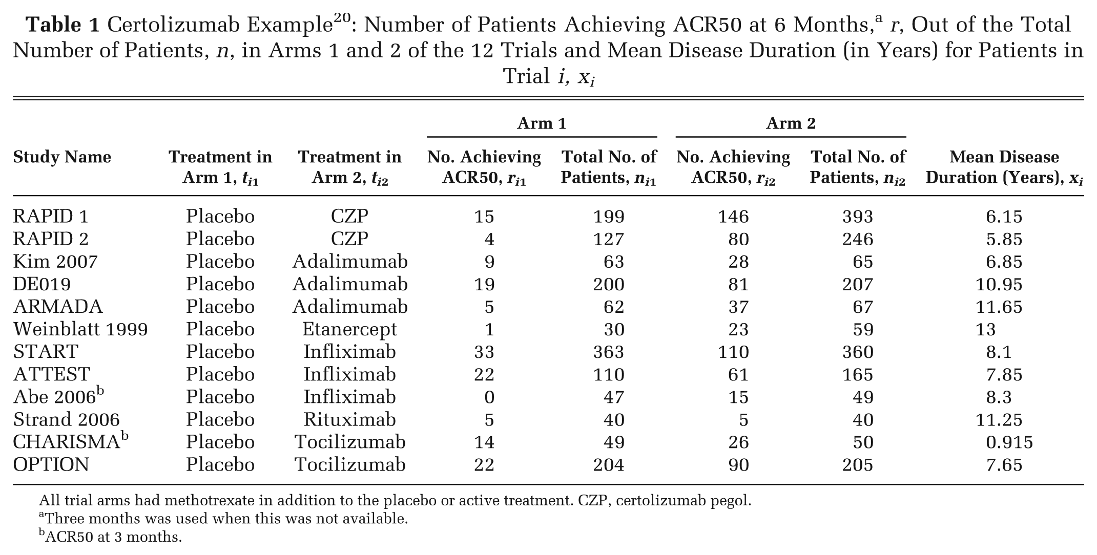
All trial arms had methotrexate in addition to the placebo or active treatment. CZP, certolizumab pegol.

Three months was used when this was not available.

ACR50 at 3 months.

Figure 3

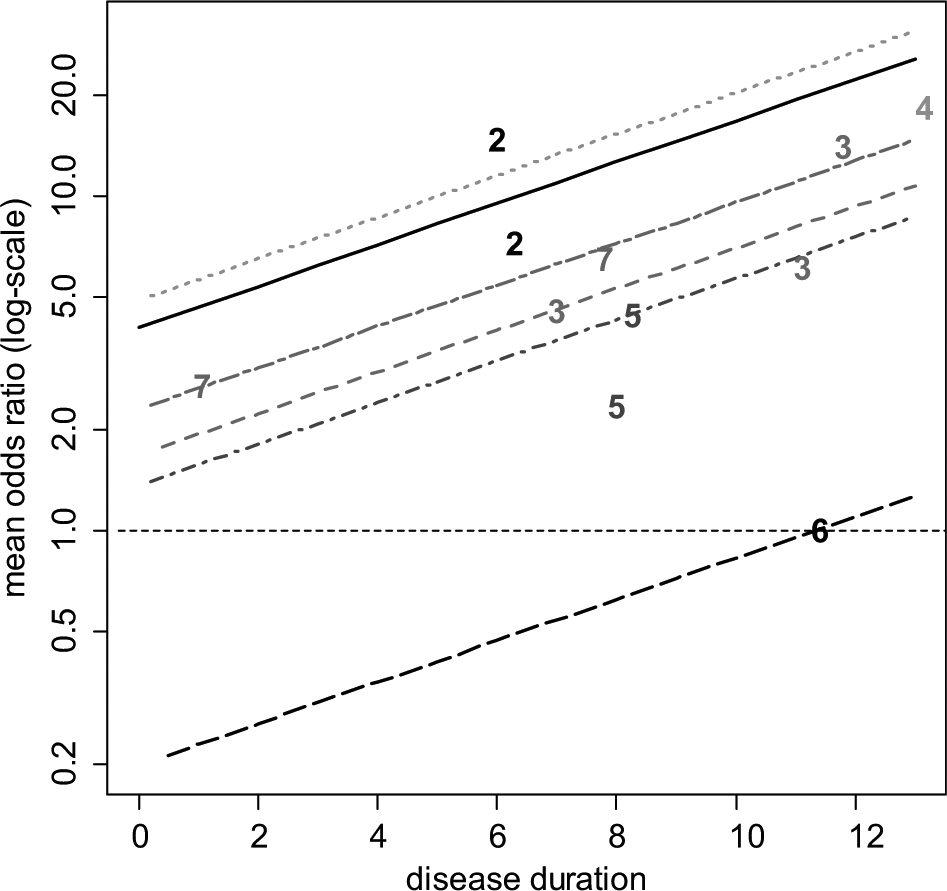
Certolizumab example²⁰: plot of the crude odds ratio (OR) (on a log-scale) of the 6 active treatments relative to placebo plus methotrexate (MTX) against mean disease duration (in years). For plotting purposes, the odds of response on placebo plus MTX for the Abe 2006 study were assumed to be 0.01. The plotted numbers refer to the treatment being compared with placebo plus MTX, and the lines represent the relative effects of the following treatments compared with placebo plus MTX based on a random effects meta-regression model (from top to bottom): etanercept plus MTX (treatment 4, dotted green line), certolizumab pegol (CZP) plus MTX (treatment 2, solid black line), tocilizumab plus MTX (treatment 7, short-long dash purple line), adalimumab plus MTX (treatment 3, dashed red line), infliximab plus MTX (treatment 5, dot-dashed dark blue line), and rituximab plus MTX (treatment 6, long-dashed black line). Odds ratios above 1 favor the plotted treatment, and the horizontal line (thin dashed) represents no treatment effect.

Table 2 shows the results of fitting fixed and random treatment effects NMA¹³ and interaction models with disease duration as the covariate. The estimated ORs for different durations of disease are represented by the parallel lines in Figure 3. Note that the treatment effects obtained are the estimated log-odds ratios at the mean covariate value ( $\bar{x} = 8.21$ years in this case) and that credible interval lines have not been included in Figure 3.

Table 2

Certolizumab Example²⁰: Posterior Mean, SD, and 95% CrI for the Interaction Estimate (b) and Log-Odds Ratios d_XY of Treatment Y relative to Treatment X

	No Covariate						Covariate “Disease Duration”
	FE			RE^a			FE			RE^a
	Mean	SD	CrI	Mean/ Median	SD	CrI	Mean	SD	CrI	Mean/ Median	SD	CrI
b	NA	NA	NA	NA	NA	NA	0.14	0.06	(0.01, 0.26)	0.14	0.09	(−0.03, 0.32)
d ₁₂	2.21	0.25	(1.73, 2.72)	2.27	0.39	(1.53, 3.10)	2.50	0.29	(1.96, 3.08)	2.57	0.42	(1.79, 3.44)
d ₁₃	1.93	0.22	(1.52, 2.37)	1.97	0.33	(1.33, 2.64)	1.66	0.25	(1.19, 2.16)	1.71	0.34	(1.04, 2.41)
d ₁₄	3.47	1.34	(1.45, 6.74)	3.46	1.41	(1.26, 6.63)	2.82	1.34	(0.71, 5.96)	2.77	1.42	(0.42, 6.01)
d ₁₅	1.38	0.17	(1.06, 1.72)	1.48	0.33	(0.90, 2.21)	1.40	0.17	(1.08, 1.74)	1.48	0.30	(0.95, 2.15)
d ₁₆	0.00	0.71	(−1.40, 1.39)	0.01	0.82	(−1.61, 1.63)	−0.42	0.73	(−1.86, 1.04)	−0.44	0.84	(−2.08, 1.21)
d ₁₇	1.65	0.22	(1.22, 2.10)	1.56	0.38	(0.77, 2.28)	1.98	0.28	(1.45, 2.53)	2.00	0.45	(1.12, 2.93)
σ	NA	NA	NA	0.34	0.20	(0.03, 0.77)	NA	NA	NA	0.28	0.19	(0.02, 0.73)
${\bar{D}}_{res}$ ^b	37.6			30.9			33.8			30.2
p_D	18.0			21.2			19.0			21.3
DIC	55.6			52.1			52.8			51.4

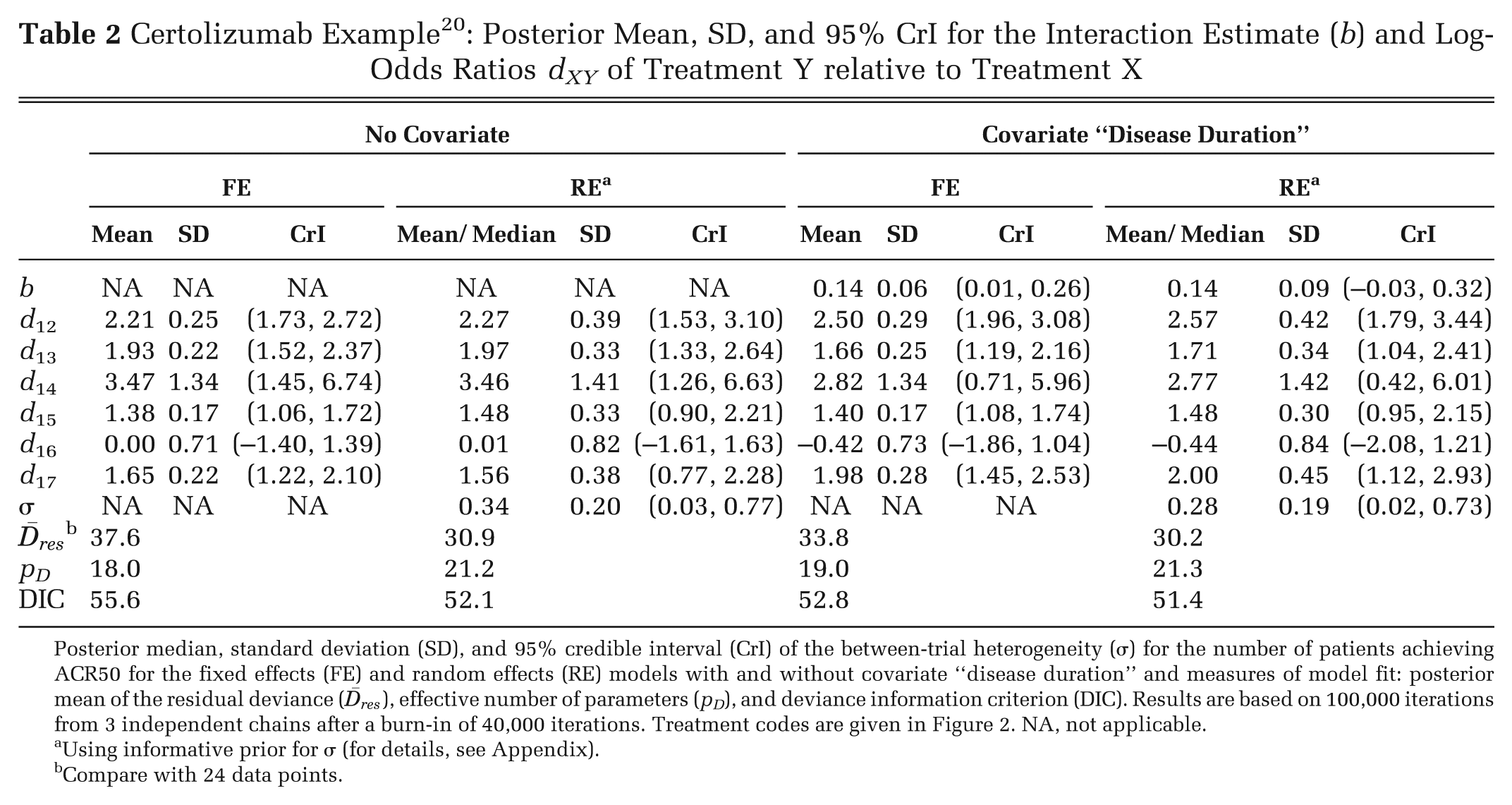
Posterior median, standard deviation (SD), and 95% credible interval (CrI) of the between-trial heterogeneity (σ) for the number of patients achieving ACR50 for the fixed effects (FE) and random effects (RE) models with and without covariate “disease duration” and measures of model fit: posterior mean of the residual deviance ( ${\bar{D}}_{res}$ ), effective number of parameters (p_D ), and deviance information criterion (DIC). Results are based on 100,000 iterations from 3 independent chains after a burn-in of 40,000 iterations. Treatment codes are given in Figure 2. NA, not applicable.

Using informative prior for σ (for details, see Appendix).

Compare with 24 data points.

The deviance information criterion (DIC) provides a measure of model fit that penalizes model complexity²²—lower values of the DIC suggest a more parsimonious model. We calculate the DIC as the sum of the posterior mean of the residual deviance, ${\bar{D}}_{res}$ , and the leverage, p_D .¹³ The DIC and posterior means of the residual deviances in Table 2 do not decisively favor a single model (differences less than 3 or 5 are not considered meaningful). The fit of the FE model is improved by including the covariate interaction term b, which also has a CrI that does not include zero. Addition of the covariate to the RE model reduces the heterogeneity from a posterior median of 0.34 to 0.28, but the CrI for the interaction parameter b includes zero. In this example, the meta-regression models are all reasonable but not strongly supported by the evidence, although the finding of smaller treatment effects with a shorter disease duration has been reported previously.¹⁸

Should the use of biologics be confined to patients whose disease duration was above a certain threshold? This seems reasonable, but it would be difficult to determine this threshold on the basis of this evidence alone. The slope is largely determined by treatments 3 and 7 (adalimumab and tocilizumab), which are the only treatments trialed at more than 1 disease duration and appear to have different effects at each duration (Figure 3). However, the linearity of relationships is highly questionable, and the prediction of negative effects for treatment 6 (rituximab) is not plausible. This suggests that other explorations of the causes of heterogeneity in this network should be undertaken (see below).

Network Meta-Regression on Baseline Risk

The meta-regression model presented above can be extended to use the baseline risk in each trial as a covariate, taking into account the error in the estimation of baseline risk and its correlation to the OR. The model is the same as in equation (4) but now x_i = µ_i, the trial-specific baseline for the control arm in each trial. An important property of this Bayesian formulation is that it takes the “true” baseline (as estimated by the model) as the covariate and automatically takes the uncertainty in each µ_i into account.^23,24 Naive approaches, which regress against the observed baseline risk, fail to take the correlation between the treatment effect and baseline risk, as well as the consequent regression to the mean phenomenon, into account.

Example: Certolizumab Meta-Regression on Baseline Risk (Appendix: Example 3)

Both FE and RE models with a common interaction term were fitted. Due to covariate centering, the treatment effects in Table 3 for the models with covariate adjustment are the effects for patients with a baseline log-odds ACR50 of −2.421, the mean of the observed log-odds on treatment 1. This corresponds to a baseline ACR50 probability of 0.082.

Table 3

Certolizumab Example²⁰: Posterior Mean, SD, and 95% CrI for the Interaction Estimate (b) and Log-Odds Ratios d_XY of Treatment Y Relative to Treatment X

	FE			RE
	Mean	SD	CrI	Mean/Median	SD	CrI
b	−0.93	0.09	(−1.03, −0.69)	−0.95	0.10	(−1.10, −0.70)
d ₁₂	1.85	0.10	(1.67, 2.06)	1.83	0.24	(1.35, 2.29)
d ₁₃	2.13	0.11	(1.90, 2.35)	2.18	0.22	(1.79, 2.63)
d ₁₄	2.08	0.34	(1.47, 2.80)	2.04	0.46	(1.19, 2.94)
d ₁₅	1.68	0.10	(1.49, 1.86)	1.71	0.22	(1.30, 2.16)
d ₁₆	0.36	0.50	(−0.72, 1.27)	0.37	0.59	(−0.86, 1.45)
d ₁₇	2.20	0.14	(1.93, 2.46)	2.25	0.27	(1.75, 2.79)
σ	NA	NA	NA	0.19	0.19	(0.01, 0.70)
${\bar{D}}_{res}$ ^a	27.3			24.2
p_D	19.0			19.4
DIC	46.3			43.6

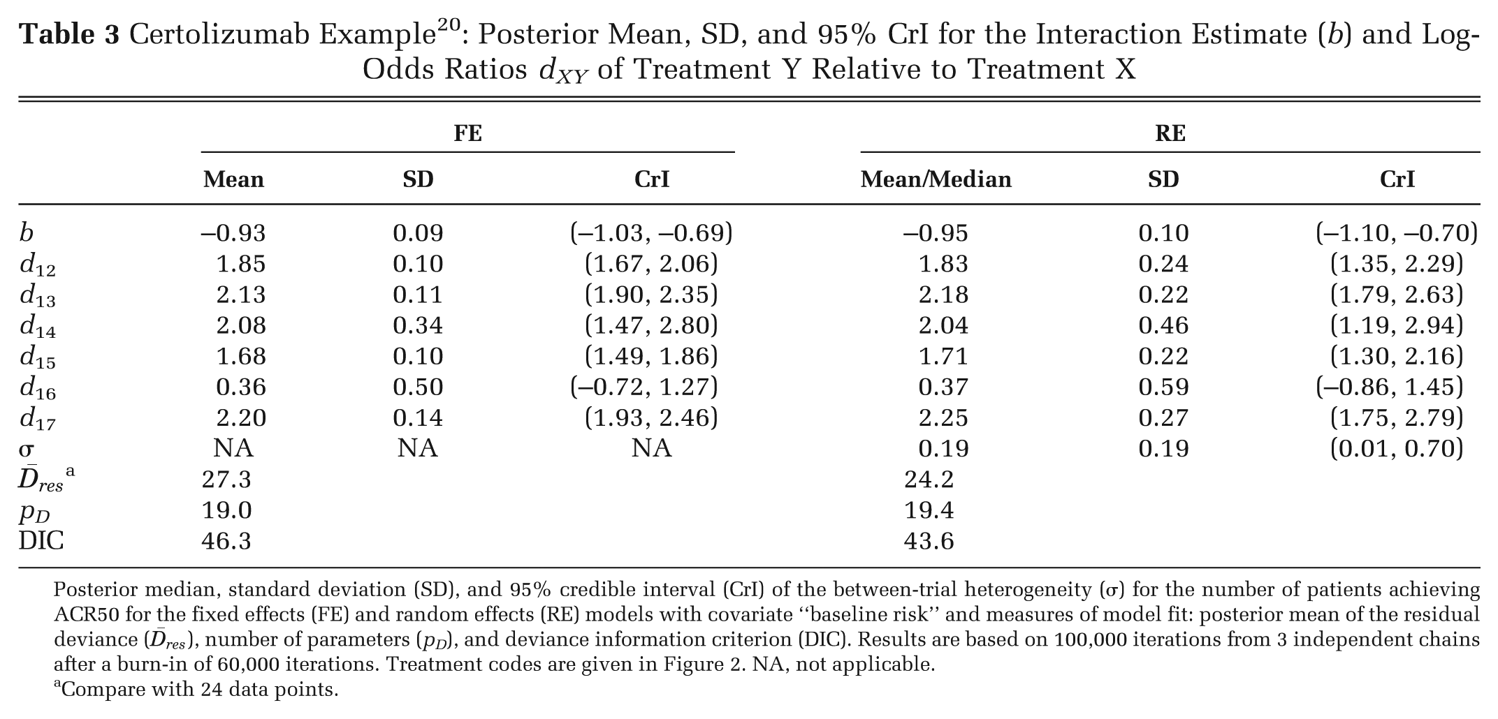
Posterior median, standard deviation (SD), and 95% credible interval (CrI) of the between-trial heterogeneity (σ) for the number of patients achieving ACR50 for the fixed effects (FE) and random effects (RE) models with covariate “baseline risk” and measures of model fit: posterior mean of the residual deviance ( ${\bar{D}}_{res}$ ), number of parameters (p_D ), and deviance information criterion (DIC). Results are based on 100,000 iterations from 3 independent chains after a burn-in of 60,000 iterations. Treatment codes are given in Figure 2. NA, not applicable.

Compare with 24 data points.

In both models, the 95% CrIs for covariate term exclude zero, suggesting a strong interaction effect between the baseline risk and the treatment effects. The estimated RE model is shown in Figure 4: the differences between the lines represent treatment differences controlling for baseline risk. However, note that there is considerable uncertainty around these lines, which is not represented in Figure 4. The DIC statistics and the posterior means of the residual deviance also marginally favor the RE model with the covariate. In interpreting the results of this model, it should be noted that treatment effect is being defined on a percent change scale: the extent of change is therefore automatically increased as the baseline is lowered. Hence, the observed interaction may to some extent be an artifact of the measurement scale.

Figure 4

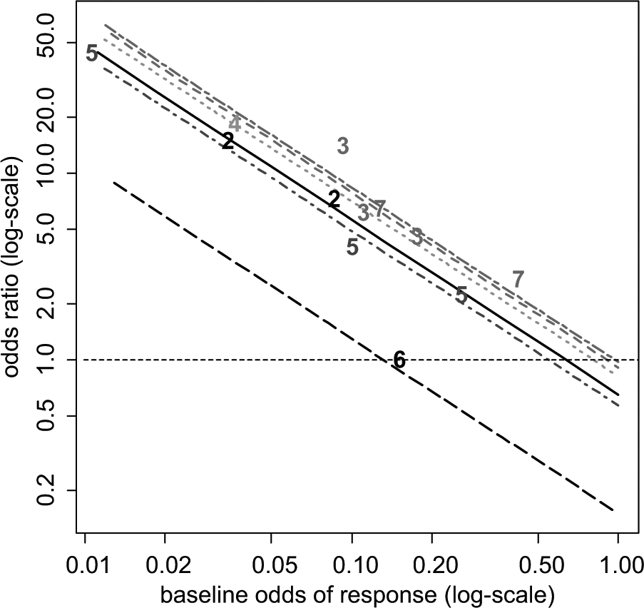
Certolizumab example²⁰: plot of the crude odds ratio (OR) of the 6 active treatments relative to placebo plus methotrexate (MTX) against odds of baseline response on a log-scale. For plotting purposes, the odds of response on placebo plus MTX for the Abe 2006 study were assumed to be 0.01. The plotted numbers refer to the treatment being compared with placebo plus MTX, and the lines represent the relative effects of the following treatments (from top to bottom) compared with placebo plus MTX based on a random effects meta-regression model: tocilizumab plus MTX (treatment 7, short-long dash purple line), adalimumab plus MTX (treatment 3, dashed red line), etanercept plus MTX (treatment 4, dotted green), certolizumab pegol (CZP) plus MTX (treatment 2, solid black line), infliximab plus MTX (treatment 5, dot-dashed dark blue line), and rituximab plus MTX (treatment 6, long-dashed black line). Odds ratios above 1 favor the plotted treatment, and the horizontal line (dashed) represents no treatment effect.

Bias and Bias-Adjustment

If it is thought that heterogeneity is due to bias in some of the included studies, models for bias-adjustment can be used. The difference between “bias-adjustment” and the meta-regression models described above is slight but important. In meta-regression, we concede that even within the formal scope of the decision problem, there are distinct differences in relative treatment efficacy. In bias-adjustment, we have in mind a target population for decision making, but the evidence available, or at least some of the evidence, provides biased, or potentially biased, estimates of the target parameter, perhaps because the trials have internal biases, they concern different populations or settings, or both.

Adjustment for Bias Based on Meta-Epidemiological Data

Confronted by trial evidence of mixed quality, investigators have 3 options: 1) to restrict attention to studies of high quality, ignoring what may be a substantial proportion of the evidence; 2) to include trials of both high and low quality in a single analysis, which risks delivering a biased estimate of the treatment effect; or 3) to use all the data but simultaneously adjust and down-weight the evidence from studies at risk of bias.²⁵ The latter uses information on the expected bias, as well as between-study variation in bias, derived from statistical analysis of meta-epidemiological data. The analysis assumes that the study-specific biases in the data set of interest are exchangeable with those in the meta-epidemiological data used to provide the prior distributions used for adjustment. This approach can form the basis for sensitivity analyses to show whether the presence of studies at risk of bias, with potentially over-optimistic results, has an impact on the decision.²⁵

It is expected that this bias-adjustment method will be used more when more data are available on how the degree of bias depends on the nature of the outcome measure and the clinical condition.⁴ In principle, the same form of bias-adjustment could be extended to other types of bias or to mixtures of RCTs and observational studies. Each of these extensions, however, depends on the applicability of analyses of very large meta-epidemiological data sets that are starting to become available.^11,26

Estimation and Adjustment for Bias in Network Meta-Analysis

In NMA, if we assume that the mean and variance of the study-specific biases are the same for each treatment, it is possible to simultaneously estimate the treatment effects and the bias effects in a single analysis and to produce treatment effects that are based on the entire body of data and also adjusted for bias.²⁷ If A is placebo or standard treatment and B, C, and D are all active treatments, it would be reasonable to expect the same bias distribution to apply to the AB, AC, and AD trials. But it is less clear what the direction of the bias should be in BC, BD, and CD trials. Assuming that the average bias is always in favor of the newer treatment, this becomes a model for novelty bias.^28,29 Another approach might be to propose a separate mean bias term for active v. active comparisons.²⁷

This method can in principle be extended to include syntheses that are mixtures of trials and observational studies, and it can also be extended to any form of “internal” bias. A particularly interesting application is to “small-study bias,” which is one interpretation of “publication bias.” The idea is that smaller studies have greater bias. The “true” treatment effect can therefore be conceived as the effect that would be obtained in a study of infinite size, which is taken to be the intercept in a regression of the treatment effect against the study variance.^30,31

Elicitation of Bias Distributions

This method³² is conceptually the simplest of all bias-adjustment methods, applicable to trials and observational studies alike, but it is also the most difficult and time-consuming. One of its advantages is that it can be used when the number of trials is insufficient for meta-regression approaches. Each study is considered by several independent experts using a predetermined protocol that itemizes a series of potential internal and external biases. Each expert is asked to provide information that is used to develop a combined bias distribution. The mean and variance of the bias distributions are statistically combined with the original study estimate and its variance to create a new, adjusted estimate of the treatment effect in each study. The final stage is a conventional synthesis of the adjusted study-specific estimates using standard pairwise or network meta-analysis methods.

Discussion

We have detailed methods to explore or explain heterogeneity in pairwise and network meta-analyses using study-level covariates, including baseline risk (variation in “baseline” natural history is dealt with in another tutorial in this series³³), although we have not covered the closely related topic of outlier detection.^16,34,35

However, meta-regression based on aggregate data and study-level covariates suffers from several bias and confounding problems as well as typically having low power. When a categorical covariate is considered, one can contrast a within-trial comparison (e.g., treatment effects reported separately for males and females) and a between-trial comparison where different trials are run on male and female patients. The contrast is similar to the difference between a paired and an unpaired t test. With between-trial comparisons, a given covariate effect (i.e., interaction) will be harder to detect as it has to be distinguishable from the “random noise” created by the between-trial variation. However, for within-trial comparisons, the between-trial variation is controlled for, and the interaction effect needs only to be distinguishable from sampling error. A further drawback of between-trial comparisons is that, because the number of observations (trials) may be very low while the precision of each trial may be relatively high, it is quite possible to observe a highly statistically significant relation between the treatment effect and the covariate that is entirely spurious.³⁶ Furthermore, between-trial comparisons are more vulnerable to ecologic bias or ecologic fallacy,³⁷ where, for example, a linear regression coefficient of treatment effect against the covariate in the between-trial case can be entirely different from the coefficient for the within-trial data.

With continuous covariates and IPD, not only does the within-trial comparison avoid ecological bias, but it also has far greater statistical power to detect a true covariate effect. This is because the variation in patient covariate values will be many times greater than the variation between the trial means,^38,39 and the precision in any estimated regression coefficient depends directly on the variance in covariate values. For these reasons, IPD meta-analyses and meta-regression are taken to be the “gold standard,”⁴⁰ although IPD is not available in most situations.

Two broad approaches to IPD meta-regression have been considered.⁴¹ In the 2-step approach, the analyst first estimates the interaction effect sizes and their standard errors from each study and then conducts a standard meta-analysis on these summaries. This is appropriate for inference on the existence of an interaction, but for decision making, we recommend a 1-step method in which main effects and interaction are estimated simultaneously. This is because the parameter estimates of the main effects and interaction terms will be correlated, and their joint uncertainty can most easily be propagated through the decision model by estimating them simultaneously. IPD RE pairwise meta-analysis models have been developed for continuous,^42,43 binary,⁴⁴ survival,⁴⁵ and ordinal⁴⁶ variables. Although most of the models are presented in the single pairwise comparison context, it is possible to extend them to an NMA context.^{42,47

–51} Criteria for determining the potential benefits of IPD to assess patient-level covariates have recently been outlined.⁵²

When IPD is available only in a subset of studies, it is possible to incorporate both types of data in the same analysis using dual effect models.^{48,50,53
–55} This makes the best possible use of all available data, but a decision has to be made on whether between-study variability is to be included in the estimation of effects. Statistical tests are unlikely to have sufficient power to inform a decision. In an NMA with IPD, we would recommend use of models with a single interaction term for each covariate, at least within a class of treatments, for decision making, but more complex structures have been attempted.⁴⁹

Finally, it needs to be appreciated that in cases where the covariate does not interact with the treatment effect but modifies the baseline risk, the effect of pooling data over the covariate is to bias the estimated treatment effect toward the null effect. This is a form of ecologic bias known as aggregation bias,³⁷ which does not affect strictly linear models, where pooling data across such covariates will not create bias. Usually, it is significant only when both the covariate effect on baseline risk and the treatment effect are quite strong. It is a particular danger in survival analysis because the effect of covariates such as age on cancer risk can be particularly marked and because the log-linear models routinely used are highly nonlinear. When covariates that affect risk are present, even if they do not modify the treatment effect, the analysis must be based on pooled estimates of treatment effects from a stratified analysis for group covariates and regression for continuous covariates and not on treatment effects estimated from pooled data.

Bias-adjustment methods are another form of accounting for differences between studies. These methods should be considered semi-experimental as there is a need for further experience with applications and for further meta-epidemiological data on the relationships between the many forms of internal bias that have been proposed.²⁹ However, they represent reasonable and valid methods for bias-adjustment and are likely to be superior to no bias-adjustment in situations where data are of mixed quality. At the same time, caution is required as the method is essentially a meta-regression based on “between-studies” comparisons, with no certainty of a causal mechanism.

We have suggested that choice between models with and without the covariate or bias-adjustment coefficients should be based on examining the DIC and the CrI of the regression coefficient. However, in general, the DIC is not able to inform choice between RE models with and without covariates as both will tend to fit equally well and have a similar effective number of parameters. Other considerations, such as a reduction in the heterogeneity, will play a greater role in choosing between RE models. For FE models with and without covariates, the DIC is suitable for model choice.

Footnotes

Appendix

Acknowledgements

We thank Jenny Dunn at NICE DSU and Julian Higgins, Jeremy Oakley, and Catrin Tudor-Smith for reviewing previous versions of this article.

This series of tutorial papers were based on Technical Support Documents in Evidence Synthesis (available from ), which were prepared with funding from the NICE Decision Support Unit. The views, and any errors or omissions, expressed in this document are of the authors only.

References

National Institute for Health and Clinical Excellence (NICE). Guide to the Methods of Technology Appraisal. London, UK: NICE; 2008.

Higgins

JPT

Green

, eds. Cochrane Handbook for Systematic Reviews of Interventions Version 5.0.0 [updated February 2008]. Chichester, UK: The Cochrane Collaboration, Wiley; 2008.

Schulz

Chalmers

Hayes

Altman

. Empirical evidence of bias: dimensions of methodological quality associated with estimates of treatment effects in controlled trials. JAMA. 1995;273(5):408–12.

Wood

Egger

Gluud

. Empirical evidence of bias in treatment effect estimates in controlled trials with different interventions and outcomes: meta-epidemiological study. BMJ. 2008;336:601–5.

Higgins

JPT

Thompson

Spiegelhalter

. A re-evaluation of random-effects meta-analysis. J R Stat Soc Ser A. 2009;172:137–59.

Ades

Higgins

JPT

. The interpretation of random effects meta-analysis in decision models. Med Decis Making. 2005;25(6):646–54.

Welton

White

Higgins

JPT

Ades

Hilden

. Correction: interpretation of random effects meta-analysis in decision models. Med Decis Making. 2007;27:212–4.

Spiegelhalter

Abrams

Myles

. Bayesian Approaches to Clinical Trials and Health-Care Evaluation. New York: John Wiley; 2004.

Thompson

. Why sources of heterogeneity in meta-analyses should be investigated. BMJ. 1994;309:1351–5.

10.

Thompson

. Why and how sources of heterogeneity should be investigated. In: Egger

Davey Smith

Altman

, eds. Systematic Reviews in Health Care: Meta-Analysis in Context. 2nd ed. London, UK: BMJ Books; 2001. p 157–75.

11.

Turner

Davey

Clarke

Thompson

Higgins

JPT

. Predicting the extent of heterogeneity in meta-analysis, using empirical data from the Cochrane Database of Systematic Reviews. Int J Epidemiol. 2012;41:818–27.

12.

Borenstein

Hedges

Higgins

JPT

Rothstein

. Introduction to Meta-Analysis. Chichester, UK: John Wiley; 2009.

13.

Dias

Sutton

Ades

Welton

. Evidence synthesis for decision making 2: a generalized linear modeling framework for pairwise and network meta-analysis of randomized controlled trials. Med Decis Making. 2013;33(5):2013;33(5):607-617.

14.

Dias

Welton

Sutton

Caldwell

Ades

. Evidence synthesis for decision making 4: inconsistency in networks of evidence based on randomized controlled trials. Med Decis Making. 2013;33(5):641-656.

15.

Sutton

. Meta-Analysis Methods for Combining Information from Different Sources Evaluating Health Interventions. Leicester, UK: University of Leicester; 2002.

16.

Dias

Sutton

Welton

Ades

. NICE DSU Technical Support Document 3: Heterogeneity: subgroups, meta-regression, bias and bias-adjustment. 2011. Available from: http://www.nicedsu.org.uk

17.

Cooper

Sutton

Morris

Ades

Welton

. Addressing between-study heterogeneity and inconsistency in mixed treatment comparisons: application to stroke prevention treatments in individuals with non-rheumatic atrial fibrillation. Stat Med. 2009;28:1861–81.

18.

Nixon

Bansback

Brennan

. Using mixed treatment comparisons and meta-regression to perform indirect comparisons to estimate the efficacy of biologic treatments in rheumatoid arthritis. Stat Med. 2007;26(6):1237–54.

19.

Draper

Smith

. Applied Regression Analysis. 3rd ed. New York: John Wiley; 1998.

20.

National Institute for Health and Clinical Excellence. Certolizumab pegol for the treatment of rheumatoid arthritis. 2010. Report No. TA186. Available from: http://guidance.nice.org.uk/TA186

21.

Lunn

Thomas

Best

Spiegelhalter

. WinBUGS—a Bayesian modelling framework: concepts, structure, and extensibility. Stat Comput. 2000;10:325–37.

22.

Spiegelhalter

Best

Carlin

van der Linde

. Bayesian measures of model complexity and fit. J R Stat Soc Ser B. 2002;64(4):583–616.

23.

McIntosh

. The population risk as an explanatory variable in research synthesis of clinical trials. Stat Med. 1996;15:1713–28.

24.

Thompson

Smith

Sharp

. Investigating underlying risk as a source of heterogeneity in meta-analysis. Stat Med. 1997;16:2741–58.

25.

Welton

Ades

Carlin

Altman

Sterne

JAC

. Models for potentially biased evidence in meta-analysis using empirically based priors. J R Stat Soc Ser A. 2009;172(1):119–36.

26.

Savovic

Harris

Wood

. Development of a combined database for meta-epidemiological research. Res Synthesis Methods. 2010;1:212–25.

27.

Dias

Welton

Marinho

VCC

Salanti

Higgins

JPT

Ades

. Estimation and adjustment of bias in randomised evidence by using mixed treatment comparison meta-analysis. J R Stat Soc Ser A. 2010;173(3):613–29.

28.

Salanti

Dias

Welton

. Evaluating novel agent effects in multiple treatments meta-regression. Stat Med. 2010;29:2369–83.

29.

Dias

Welton

Ades

. Study designs to detect sponsorship and other biases in systematic reviews. J Clin Epidemiol. 2010;63:587–8.

30.

Moreno

Sutton

Ades

. Assessment of regression-based methods to adjust for publication bias through a comprehensive simulation study. BMC Med Res Methodol. 2009;9:2.

31.

Moreno

Sutton

Turner

. Novel methods to deal with publication biases: secondary analysis of antidepressant trials in the FDA trial registry database and related journal publications. BMJ. 2009;339:b2981.

32.

Turner

Spiegelhalter

Smith

GCS

Thompson

. Bias modelling in evidence synthesis. J R Stat Soc Ser A. 2009;172:21–47.

33.

Dias

Welton

Sutton

Ades

. Evidence synthesis for decision making 5: the baseline natural history model. Med Decis Making. 2013;33(5):657-670.

34.

Madan

Stevenson

Ades

Cooper

Whyte

Akehurst

. Consistency between direct and indirect trial evidence: is direct evidence always more reliable? Value Health. 2011;14:953–60.

35.

Welton

Sutton

Cooper

Abrams

Ades

. Evidence Synthesis for Decision Making in Healthcare. New York: John Wiley; 2012.

36.

Higgins

JPT

Thompson

. Controlling the risk of spurious findings from meta-regression. Stat Med. 2004;23:1663–82.

37.

Rothman

Greenland

Lash

. Modern Epidemiology. 3rd ed. Philadelphia, PA: Lippincott, Williams & Wilkins; 2008.

38.

Lambert

Sutton

Abrams

Jones

. A comparison of summary patient-level covariates in meta-regression with individual patient data meta-analysis. J Clin Epidemiol. 2002;55:86–94.

39.

Berlin

Santanna

Schmid

Szczech

Feldman

. Individual patient- versus group-level data meta-regressions for the investigation of treatment effect modifiers: ecological bias rears its ugly head. Stat Med. 2002;21:371–87.

40.

Stewart

Clarke

. Practical methodology of meta-analyses (overviews) using updated individual patient data. Stat Med. 1995;14:2057–79.

41.

Simmonds

Higgins

JPT

Stewart

Tierney

Clarke

Thompson

. Meta-analysis of individual patient data from randomized trials: a review of methods used in practice. Clin Trials. 2005;2:209–17.

42.

Higgins

JPT

Whitehead

Turner

Omar

Thompson

. Meta-analysis of continuous outcome data from individual patients. Stat Med. 2001;20:2219–41.

43.

Goldstein

Yang

Omar

Turner

Thompson

. Meta-analysis using multilevel models with an application to the study of class size effects. Appl Stat. 2000;49:399–412.

44.

Turner

Omar

Yang

Goldstein

Thompson

. A multilevel model framework for meta-analysis of clinical trials with binary outcomes. Stat Med. 2000;19:3417–32.

45.

Tudor Smith

Williamson

Marson

. Investigating heterogeneity in an individual patient data meta-analysis of time to event outcomes. Stat Med. 2005;24:1307–19.

46.

Whitehead

Omar

Higgins

JPT

Savaluny

Turner

Thompson

. Meta-analysis of ordinal outcomes using individual patient data. Stat Med. 2001;20:2243–60.

47.

Tudor Smith

Marson

Chadwick

Williamson

. Multiple treatment comparisons in epilepsy monotherapy trials. Trials. 2007;8:34.

48.

Achana

Cooper

Dias

. Extending methods for investigating the relationship between treatment effect and baseline risk from pairwise meta-analysis to network meta-analysis. Stat Med. 2013;32:752–71.

49.

Saramago

Sutton

Cooper

Manca

. Mixed treatment comparisons using aggregate and individual participant level data. Stat Med. 2012;31:3516–36.

50.

Donegan

Williamson

D’Alessandro

Garner

Tudor Smith

. Combining individual patient data and aggregate data in mixed treatment comparison meta-analysis: individual patient data may be beneficial if only for a subset of trials. Stat Med. 2013;32:914–30.

51.

Donegan

Williamson

D’Alessandro

Tudor Smith

. Assessing the consistency assumption by exploring treatment by covariate interactions in mixed treatment comparison meta-analysis: individual patient-level covariates versus aggregate trial-level covariates. Stat Med. 2012;31:3840–57.

52.

Simmonds

Higgins

JPT

. Covariate heterogeneity in meta-analysis: criteria for deciding between meta-regression and individual patient data. Stat Med. 2007;26:2982–99.

53.

Riley

Abrams

Lambert

Sutton

Thompson

. An evaluation of bivariate random-effects meta-analysis for the joint synthesis of two correlated outcomes. Stat Med. 2007;26:78–97.

54.

Riley

Lambert

Staessen

Wang

Gueyffier

Boutitie

. Meta-analysis of continuous outcomes combining individual patient data and aggregate data. Stat Med. 2008;27:1870–93.

55.

Sutton

Kendrick

Coupland

CAC

. Meta-analysis of individual- and aggregate-level data. Stat Med. 2008;27:651–69.

56.

Dias

Welton

Sutton

Ades

. NICE DSU Technical Support Document 2: A generalised linear modelling framework for pair-wise and network meta-analysis of randomised controlled trials. 2011. Available from: http://www.nicedsu.org.uk

Evidence Synthesis for Decision Making 3

Abstract

Keywords

Subgroup Effects (Appendix: Example 1)

Meta-Regression Models in Network Meta-Analysis

1. Unrelated Treatment-Specific Interactions

2. Exchangeable and Related Treatment-Specific Interactions

3. Same Interaction Effect for All Treatments

Network Meta-Regression with a Continuous Covariate

Example: Certolizumab Meta-Regression on Mean Disease Duration (Appendix: Example 2)

Network Meta-Regression on Baseline Risk

Example: Certolizumab Meta-Regression on Baseline Risk (Appendix: Example 3)

Bias and Bias-Adjustment

Adjustment for Bias Based on Meta-Epidemiological Data

Estimation and Adjustment for Bias in Network Meta-Analysis

Elicitation of Bias Distributions

Discussion

Footnotes

Appendix

Acknowledgements

References