Simultaneous measurement of water transport across the blood–brain and blood–CSF barrier in the human brain with arterial spin labeling MRI

Abstract

Previously, water exchange across the blood–brain barrier (BBB) and blood–cerebrospinal barrier (BCSFB) was assessed by multi-delay, multi-echotime (TE) arterial spin labeling, albeit in separate acquisitions with different settings. In this study, we present a protocol for simultaneous measurement of BBB and BCSFB water exchange using a multi-TE 3D-GRASE acquisition combined with T₂-preparation. We evaluate several modeling approaches, comparing two- and three-compartment models to estimate water exchange rates from blood to gray matter (K_bl_→ GM), and to CSF (K_bl_→ CSF). ASL signal was consistent with expectations: at early time points, signal decayed rapidly across TEs in blood and GM, whereas at later time points decay was slower, consistent with label accumulation in CSF. All models yielded CBF and ATT values consistent with literature. K_bl_→ CSF was highest in the choroid plexus (≈1.75 × 10⁻² s^–1), with lower values in GM and subarachnoid space (≈1.4 × 10⁻² s^–1), and white matter (≈1.2 × 10⁻² s^–1) ROIs. In contrast, K_bl_→ GM was homogenous across the brain. The three-compartment model yielded similar Akaike Information Criterion values to the two-compartment model, but allows more insight into physiology and is thus preferred. Overall, the protocol allowed simultaneous characterization of BBB and BCSFB dynamics, with the three-compartment model offering the most informative representation of water exchange.

Keywords

Arterial spin labeling blood–brain barrier blood–CSF barrier brain clearance glymphatics MRI water exchange

Introduction

The blood–brain barrier (BBB) and blood–cerebrospinal fluid barrier (BCSFB) are vital structures of the human brain which protect neuronal tissue from harmful pathogens, regulate the transport of metabolic, immunologic, and hormonal molecules between fluids and tissues to preserve homeostasis, and facilitate the clearance of waste products.^1–4 The BBB refers to the set of membranes and junctions which form the boundary between blood and tissue found throughout the brain, while the BCSFB refers to the boundary between blood and CSF. The main exchange between blood and CSF is traditionally understood to occur at the choroid plexus (CP), a small structure located within the ventricles. The BCSFB is also implicated in the process of brain waste clearance by regulating the exchange of water and waste products between the blood and CSF. Disruptions in the function of the BBB and BCSFB are involved in a wide variety of neurological disorders such as Alzheimer’s disease, stroke, small-vessel disease, hydrocephalus, as well as the brain’s aging process.^4–12 Therefore, assessing the function of the BBB and BCSFB provides crucial information about brain health and progression of brain diseases and preferably one would like to assess both barriers at the same time, because of the close interactions between blood water, CSF, and interstitial fluid (ISF).

Traditionally, MRI measurements of BBB and BCSFB leakage are performed using gadolinium-based contrast agents (Gd), however there are limitations to these techniques. Firstly, they are invasive, measuring the leakage rate of intravenously injected Gd across the BBB¹³ or the perivascular influx of Gd after intrathecal injection.^14,15 For the latter, injections directly into the CSF may also disturb the equilibrium of the system we aim to characterize.¹⁶ Secondly, Gd crosses the barriers at a very slow rate unless there is substantial disruption to the tight junctions of the endothelial cells at the BBB and the epithelial cells at the BCSFB, which regulate the paracellular movement of Gd.^17,18 Whilst Gd has been found to cross the barriers at measurable levels in several neurodegenerative diseases as well as in the aging brain,^13,19–25 using a smaller tracer may offer improved sensitivity to subtle or early-stage barrier impairment. Additionally, contrast-enhanced techniques cannot detect damage to other transport routes across the barrier, as Gd exclusively traverses via paracellular pathways. There is also a growing concern with the deposition of Gd in the brain over time from repeated contrast injections. Therefore, there has been increasing interest in using water as an endogenous contrast medium to measure BBB and BCSFB function as it is fully non-invasive, has the potential to provide measurements of more subtle disruptions in function, and represents healthy physiology, that is, existing processes of exchange which are naturally present in the brain.

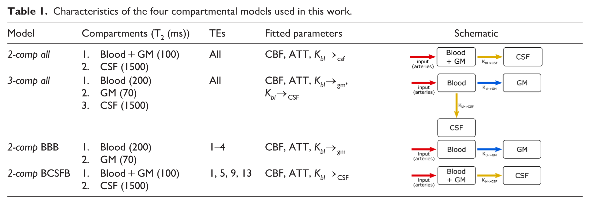
Most of the proposed methods to assess water transport across the BBB and BCSFB employ arterial spin labeling (ASL) MRI,^26–31 a technique which is generally used to measure cerebral perfusion. By optimizing ASL labeling parameters and readout strategies, blood water can be tracked as it traverses from large vessels into the tissue or CSF. Because of the different nature of the tissues and fluids involved, different techniques are used for the assessment of the integrity of the BBB and BCSFB. In all cases, multiple labeling durations (LD) and/or post-labeling delays (PLD) are employed to capture the dynamic process and either multiple echo times (TE) or different levels of flow-crushing are performed to determine in what compartment the label resides. When exploiting the difference in T₂ between compartments, the technique of choice to characterize the BBB is the combination of time-encoding with a T₂-preparation (T_2prep) module.^29,32–34 Time-encoding (or Hadamard encoding) is an efficient method for acquiring multiple LD/PLDs, especially short ones like those required for BBB imaging (~200–2000 ms). T_2prep offers the advantage of allowing flexible effective echo times (eTEs), however it considerably increases scan time as only one eTE can be acquired per TR. For BBB water transport measurements, conventionally four short (<200 ms) eTEs are acquired. For BCSFB water exchange, we have previously proposed to use separate scans with different LD/PLDs in combination with a multi-TE gradient and spin-echo (GRASE) readout.²⁸ For this method, longer LD/PLDs (~500–4000 ms) are acquired as water exchange from blood to CSF is believed to occur more slowly and to a lesser extent than exchange from blood to GM.²⁸ Consequently, Hadamard encoding was found not very efficient and did not significantly reduce scan time. To isolate water signal in the CSF, extra-long TEs (>500 ms) must be acquired as CSF has a very long T₂, which makes multi-TE GRASE an effective readout option. It has the advantage of acquiring multiple TEs simultaneously in one TR, albeit with longer inter-echo spacing. These long TE spacings (~260 ms in our previous work) do not allow proper separation of blood and GM signal because of their relatively short and similar T₂s. In this work, we aim to reconcile the advantages and disadvantages of these two techniques (see Table 1) to measure blood water exchange to both GM and CSF in a single scan. In order for our protocol to contain a wide range of both TEs and PLDs, we combined T_2prep and a multi-echo GRASE readout into one sequence and sequentially acquired multiple LD/PLDs.

Table 1.

Characteristics of the four compartmental models used in this work.

Model	Compartments (T₂ (ms))	TEs	Fitted parameters
2-comp all	1. Blood + GM (100) 2. CSF (1500)	All	CBF, ATT, K_bl_→ csf
3-comp all	1. Blood (200) 2. GM (70) 3. CSF (1500)	All	CBF, ATT, K_bl_→ gm, K_bl_→ CSF
2-comp BBB	1. Blood (200) 2. GM (70)	1–4	CBF, ATT, K_bl_→ gm
2-comp BCSFB	1. Blood + GM (100) 2. CSF (1500)	1, 5, 9, 13	CBF, ATT, K_bl_→ CSF

This study’s aims are therefore twofold:

• To investigate the use of a combination of T_2prep and multi-TE acquisition for measurement of ASL signal at both intermediate and long TEs.

• To compare the use of two- and three- compartment models tailored to differentiate the contributions from several compartments (blood, GM, or CSF) to the ASL-signal for characterization of water transport both from blood-to-GM (BBB) as well as from blood-to-CSF (BCSFB).

Methods

MRI acquisition

Data was acquired from six healthy volunteers (1 M/5 F, age 21–63) on a Philips Achieva XT 3 T system (Philips, Best, the Netherlands) with a 32-channel head coil. This study was approved by the Medisch Etische Toetsingscommissie (METC), Leiden–Den Haag–Delft. The main imaging sequence in this protocol is a pseudo-continuous ASL (PCASL) scan with multi-echo 3D GRASE readout (as described in our previous work²⁸), with the addition of a T_2prep module before readout. Here, the multi-TE readout has been shortened to four TEs acquired sequentially (TE = 10 + n × 209 ms, n = 0:3). The TSE factor was 80, the slice oversampling factor 1.8, and the in-plane acquisition matrix was 64 × 60 (RL × AP), reconstructed to a volume of 80 × 80 × 28 voxels of 3 × 3 × 6 mm³. The EPI readout in the phase-encoding direction (AP) was divided into four segments (15 lines/segment). A T_2prep module was incorporated to increase the sampling density of the T₂ decay curve, allowing more effective separation of tissue signals—particularly blood and GM, which have rather similar T₂ values and therefore require closer effective echo times to be distinguished. Four T_2prep modules were applied with lengths of 0 (no T_2prep), 40, 80, and 160 ms. These were cycled along the dynamics, that is, the acquisition of echoes was interleaved: in the first dynamic (eTE = 0), TEs = 10 + n × 209 ms, n = 0:3 (i.e. TEs #1,5,9,13) were acquired, in the second dynamic (eTE = 40), TEs = 50 + n × 209 ms, n = 0:3 (TEs #2,6,10,14), and so on, for a total of 16 TEs (10, 50, 90, 170, 219, 259, 299, 379, 428, 468, 508, 588, 637, 677, 717, and 797 ms). This represents a good compromise between short-TE and long-TE acquisitions to allow distinction between the three main compartments of interest (blood, GM and CSF). In order to keep the effective length of the PLD the same between different T_2preps, the module was inserted after the PLD (see Figure 1). Two background suppression (BGS) pulses were applied and their timings were optimized to minimize background signal from GM, white matter (WM), and CSF at the end of the PLD and before the T_2prep module. The sequence was repeated five times with variable LD/PLDs (1/0.5, 1/1, 1.5/1.5, 2/2, 4/3 s) to cover a range of timings from the arrival of blood in the voxel to the transport of water into the CSF. Repetition times (TR) were minimized for the different durations of the ASL preparation (TR = 3000, 3500, 4500, 5500, 8500 ms, respectively). Finally, an M0 scan was acquired with the same imaging parameters as the PCASL scans, but without labeling. This scan included a single TE of 10 ms and a TR of 10,000 ms (to ensure the full recovery of the GM signal). The length of individual PCASL scans varied from 6:42 to 19:00 min and the total length of this protocol was ~1 h. To avoid order-effects, we randomized the order of the PCASL scans in each participant.

Figure 1.

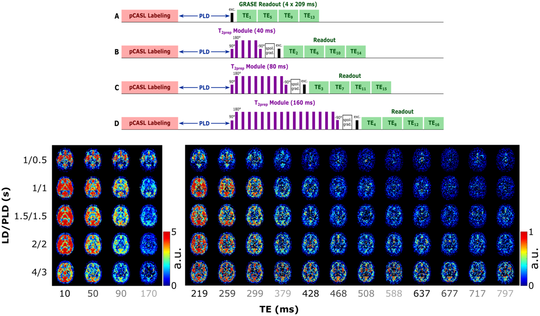
(Above) Schematic representation of the PCASL sequence used in this work. The image is not to scale (e.g. the length of the echoes in the multi-TE readout is longer than the longest T_2prep module). Each of the T_2prep module lengths (A–D) is acquired in a separate dynamic, resulting in an interleaved echo acquisition. (Below) ASL signal in a single slice for all LD/PLDs and TEs. Different scales allow the contrast to be preserved in the longer TEs. Echo times that are acquired sequentially within one readout are shown with the same grayscale intensity to highlight the interleaved acquisition.

This research was carried out in accordance with our institution’s IRB regulations (Medisch Etische Toetsingscommissie (METC), Leiden–Den Haag–Delft) and the Declaration of Helsinki.

Analysis pipeline

ASL control and label images were pair-wise subtracted to calculate ASL signal at all LD/PLDs and TEs. A CSF mask was created by thresholding the control image at the longest TE, and a GM mask was obtained by thresholding the ASL signal of the LD/PLD 2/2 s image (the closest to typical ASL perfusion parameters where there is maximal contrast between the GM and other tissues and fluids). The thresholds for these masks were adjusted for each subject by an experienced observer (first author who had 4 years of experience with ASL-data) to retain as much as possible the anatomical features such as the cortex gyri and CSF-filled sulci. The WM mask was isolated by removing the GM and CSF mask voxels from a whole brain mask. Finally, a CP mask was obtained by isolating the posterior part of the ventricles where the CP is predominantly located and using the same threshold as the GM mask to exclude the CSF surrounding the CP.

Two ROIs were created by superimposing an elliptical shape onto (1) a single slice in the middle of the brain (slice 15), comprising the majority of the left MCA territory and avoiding the ventricles (left MCA ROI) and (2) in a high slice of the brain (slice 22), comprising most of the left hemisphere in that slice (high slice ROI). The ASL signals from these ROIs were averaged, combining signal from all tissues and fluids within the elliptical regions, and four multi-compartmental models, detailed in the following section, were fitted to the resulting data. In addition, voxelwise fitting of these models was performed to generate whole-brain maps of the corresponding model parameters. Prior to fitting, the ASL signal was smoothed with a gaussian kernel (3 × 3 voxels, σ = 2 voxels) to reduce noise. To enable comparison of parameter values across brain regions, the estimated parameters were averaged within the following tissue region ROIs: GM (GM mask slice 15 and up), subarachnoid space (SAS; CSF mask slice 15 and up, excluding the ventricles), CP (CP mask), and WM (WM mask, used as a control region). Because of the small number of subjects (i.e. low statistical power), the parameters were compared qualitatively instead of performing formal statistical analyses.

Compartmental models

Four models were used to characterize the exchange of water between the blood, GM, and CSF compartments in this study. Detailed equations for the models can be found in the Supplementary Material. In brief, the first model (2-comp all) is comprised of two compartments, where the blood and GM are combined into one compartment with an intermediate T₂, and the CSF is the other. This is the same model that was used in our previous work on BCSFB characterization,²⁸ and it was chosen at the time because of the difficulty in separating the blood and GM into distinct signals because of their short and similar TEs (~200 and 70 ms, respectively) compared to the echo time spacing of ~260 ms in that study. Here, we have shorter inter-echo spacing, and the restriction to two compartments should prove unnecessary (this model was however included here for comparison to our previous data). The second model (3-comp all) is a three-compartment model with blood, GM, and CSF in separate compartments. The third and fourth models attempt to single out water exchange across the BBB and BCSFB, respectively, by fitting only a subset of the TEs. These resemble acquisitions focused on measuring either BBB or BCSFB measurements and serve as a reference against which to compare the results of our combined sequence. The third model (2-comp BBB) is a two-compartment model with the blood and GM as compartments, ignoring the CSF signal. This model only uses the first four echo times (i.e. first GRASE echo for the different T_2prep modules) since blood and GM signal mostly contributes to the signal of the shorter TEs. The fourth model (2-comp BCSFB) is a two-compartment model, with the same compartments and equations as the first model. The difference with this model is that it only includes the four GRASE TEs of the first dynamic (i.e. the four TEs acquired sequentially within one readout without a preceding T_2prep module). These last two models not only allowed us to test the use of fewer TEs for BBB and BCSFB quantification, but also focus on a single method for acquisition of multiple TEs (T_2prep and multi-TE readout, respectively), so that any errors resulting from the combination of the two are avoided. Table 2 summarizes the characteristics of the four models: the assumed T₂s^35–37 of the compartments, which TEs are used, a list of the fitted parameters, and a schematic representation of the exchange mechanics. We modeled only the unidirectional exchange of water from the blood towards other compartments, as any ASL-signal originating from water that has exchanged back into the blood should be negligible (both because it represents a very small fraction of signal, and because it would necessitate longer LD/PLD). For all models, the T₁s of blood, GM, and CSF are assumed to be 1650,³⁸ 1200,³⁷ and 4300³⁹ ms, respectively, and the inversion efficiency (α) is set equal to 0.85 (combination of the labeling efficiency⁴⁰ and the BGS pulses inversion efficiency⁴¹). A single average M0 value was calculated for each subject by averaging the signal of the M0 scan over the GM mask and dividing it by the blood–brain partition coefficient, λ = 0.98 ml/g.⁴²

Table 2.

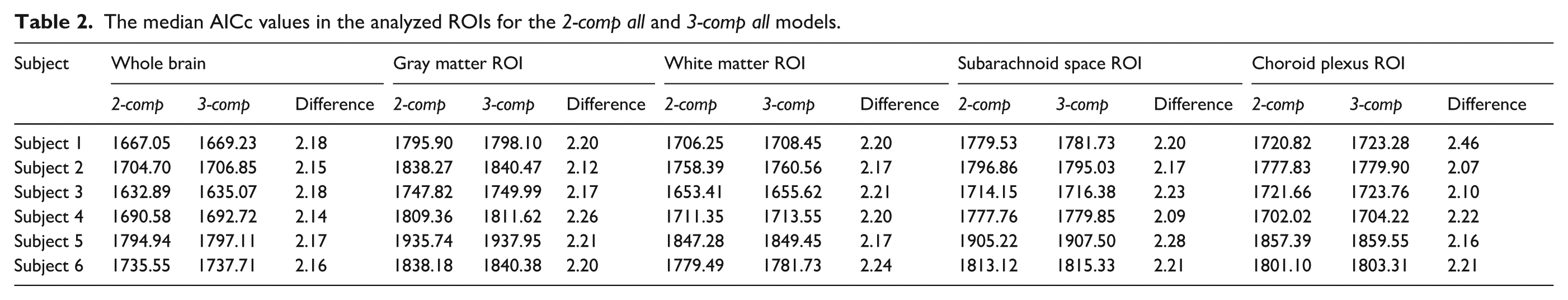
The median AICc values in the analyzed ROIs for the 2-comp all and 3-comp all models.

Subject	Whole brain			Gray matter ROI			White matter ROI			Subarachnoid space ROI			Choroid plexus ROI
	2-comp	3-comp	Difference	2-comp	3-comp	Difference	2-comp	3-comp	Difference	2-comp	3-comp	Difference	2-comp	3-comp	Difference
Subject 1	1667.05	1669.23	2.18	1795.90	1798.10	2.20	1706.25	1708.45	2.20	1779.53	1781.73	2.20	1720.82	1723.28	2.46
Subject 2	1704.70	1706.85	2.15	1838.27	1840.47	2.12	1758.39	1760.56	2.17	1796.86	1795.03	2.17	1777.83	1779.90	2.07
Subject 3	1632.89	1635.07	2.18	1747.82	1749.99	2.17	1653.41	1655.62	2.21	1714.15	1716.38	2.23	1721.66	1723.76	2.10
Subject 4	1690.58	1692.72	2.14	1809.36	1811.62	2.26	1711.35	1713.55	2.20	1777.76	1779.85	2.09	1702.02	1704.22	2.22
Subject 5	1794.94	1797.11	2.17	1935.74	1937.95	2.21	1847.28	1849.45	2.17	1905.22	1907.50	2.28	1857.39	1859.55	2.16
Subject 6	1735.55	1737.71	2.16	1838.18	1840.38	2.20	1779.49	1781.73	2.24	1813.12	1815.33	2.21	1801.10	1803.31	2.21

Akaike Information Criterion (AIC) analysis

The 2-comp all and 3-comp all model fits were compared using the small sample size corrected Akaike Information Criterion (AIC), calculated as^43–45:

A I C c = 2 k_{m} - 2 (M L L) + \frac{2 k_{m} (k_{m} + 1)}{n - k_{m} - 1}

where n is the number of data points (n_{3-comp all} = n_{2-comp all} = 5 PLDs × 16 TEs = 80), k_m is the number of estimated model parameters (for the 2-comp all model these are CBF, ATT, K_bl_→ CSF so k_m_{,2-comp all} = 3, for the 3-comp all model K_bl_→ GM is also included so k_m_{,3-comp all} = 4) and MLL is the maximum value of the log-likelihood for the model given by:

M L L = - \frac{n}{2} \ln (\frac{R S S}{n})

where RSS is the residual sum of squares. Voxelwise AIC values were evaluated across the whole brain, GM, CP, SAS, and WM ROIs.

Results

ASL signal

The measured ASL signal (Figure 1) is consistent with literature and previous work (note that two different scales are used for the first four echoes and the rest, to visualize contrast at long TEs where the signal is low). When focusing on the first TE (first column) we see the early arrival of blood in the vasculature in the first time point, then the signal appears in the GM as a perfusion pattern (LD/PLD 1/1–2/2 s) before fading away. In longer TEs (>500 ms), the CSF signal becomes apparent, with a slower inflow (it appears mostly from LD/PLD 2/2 s and longer) and slow decay through the TEs. The evolution of the signal through the TEs shows rapid decrease for blood and GM signals and slower decay in the CSF (CP and SAS). As seen in our previous work,²⁸ CSF signal from blood-to-CSF water exchange is present throughout the brain, and not exclusively in the choroid plexus.

Signal fractions

Using the parameter maps estimated from all compartmental models, the amount of signal arising from each compartment can be calculated from the model equations. These signal fractions are shown in Figure 2 for a single slice of subject 5 for all LD/PLD pairs of this study. Results of the 2-comp all and 2-comp BCSFB models are similar, and comparable to the results of our previous work using this same model. The 2-comp all, 3-comp all, and 2-comp BCSFB models result in comparable CSF signals in terms of timing, location, and intensity, with the 3-comp all model showing the highest CSF signal.

Figure 2.

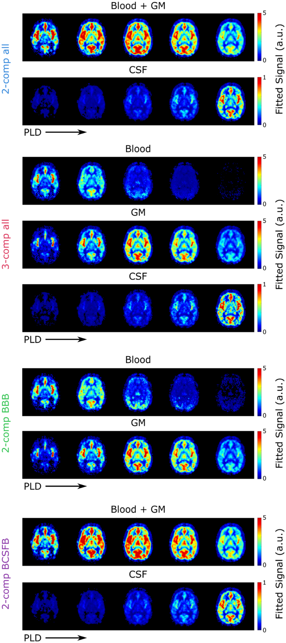
Relative amount of signal present in each compartment at TE = 10 ms and all LD/PLDs used in this experiment as fitted with the four models.

In our previous work, the blood and GM compartments were combined into a single compartment, because the large inter-echo spacing of the data did not allow their short T₂s to be distinguished and hence resulted in a large amount of overlap between their signal maps when using a three-compartment model. Here, in the 3-comp all model maps, there is some residual overlap between the two compartments, but the resulting maps show distinct patterns for blood and GM, for example, there is very little signal in the GM in the first time point, by the second time point the blood signal has completely disappeared from the large arteries, and the signal decay through time is much faster in blood than GM. However, in the second time point, the GM signal appears paradoxically more concentrated around blood vessels and the blood signal is more spread out. The overlap between blood and GM is greater in the 2-comp BBB model than the 3-comp all model.

Supplementary Figure S1 presents residual maps illustrating the differences between the total fitted signal and the measured signal at each TE/PLD for both the 2-comp all and 3-comp all models, for all subjects. Both models exhibit low residuals at longer TEs but show higher residuals at shorter TEs. This is expected, as early TEs capture signal contributions from all compartments, while at later TEs, the CSF signal becomes more isolated, as signals from blood and GM have already undergone significant T₂ decay. Variations across PLDs are also evident: the 3-comp all model tends to overestimate total signal at shorter PLDs and underestimate at longer PLDs, whereas the 2-comp all model generally overestimates at longer PLDs. These trends were consistent across different imaging slices.

Additionally, Supplementary Figure S2 shows a video of the signal obtained from the 3-comp all model for an artificial bolus of LD = 3 s for PLDs varying from 0 to 5 s. This shows a more intuitive view of the exchange of water between the three compartments, with a single (virtual) LD and therefore a smoother transition in time.

AIC results

As shown in Table 2 and Supplementary Figure S3, the AIC values for the 2-comp all model are consistently lower across all regions than the 3-comp all model. However, the differences in their AIC values are minimal, with the largest observed difference in median AIC being 2.46.

ROI analyses: Left MCA and high slice ROIs

Figure 3 shows the fit of the four different models for the left MCA ROI and high slice ROI. While both ROIs combine a mixture of signal from blood, GM, and CSF, because of the geometry of acquisition the high slice ROI contains more SAS CSF than the MCA ROI. Based on the GM, WM, and CSF masks, 45% of the voxels in the left MCA ROI contained GM, 37% contained WM, and 22% CSF. For the high slice ROI, the proportions shift to 36% GM, 46% WM, and 27% CSF. Looking at the signal curves, we see earlier arrival of the signal in the MCA territory and generally higher signal intensity. In the MCA ROI, the CBF is higher, the ATT shorter, K_bl_→ GM larger and K_bl_→ CSF smaller, consistent with the closer proximity to the circle of Willis and higher fraction of GM. In both ROIs, by visual inspection of the fitted curves the first model (2-comp all) shows lower correspondence with the data, especially for the shorter echo times (50–170 ms), than the 3-comp all model which shows a better fit at these echo times. Compared to the 3-comp-all model, 2-comp BBB overestimates CBF, and 2-comp all/2-comp BCSFB underestimate it, and the same is true for ATT. Differences between signal fractions are subtle, but we can see when comparing the 3-comp all model to 2-comp BBB that in the latter case, the CSF signal appears to be absorbed into both the GM and blood compartments as both show increased signal. In the case of the 2-comp all and 2-comp BCSFB models, some of the CSF signal appears to be absorbed into the blood + GM compartment as the fraction of CSF-signal here is lower than in the 3-comp all. From visual assessment of the fits, the 2-comp BBB model performs better in the MCA territory ROI than in the high slice ROI, because of the higher GM proportion here. On the contrary, the 2-comp BCSFB performs better in the high slice ROI, due to a greater percentage of CSF in this ROI.

Figure 3.

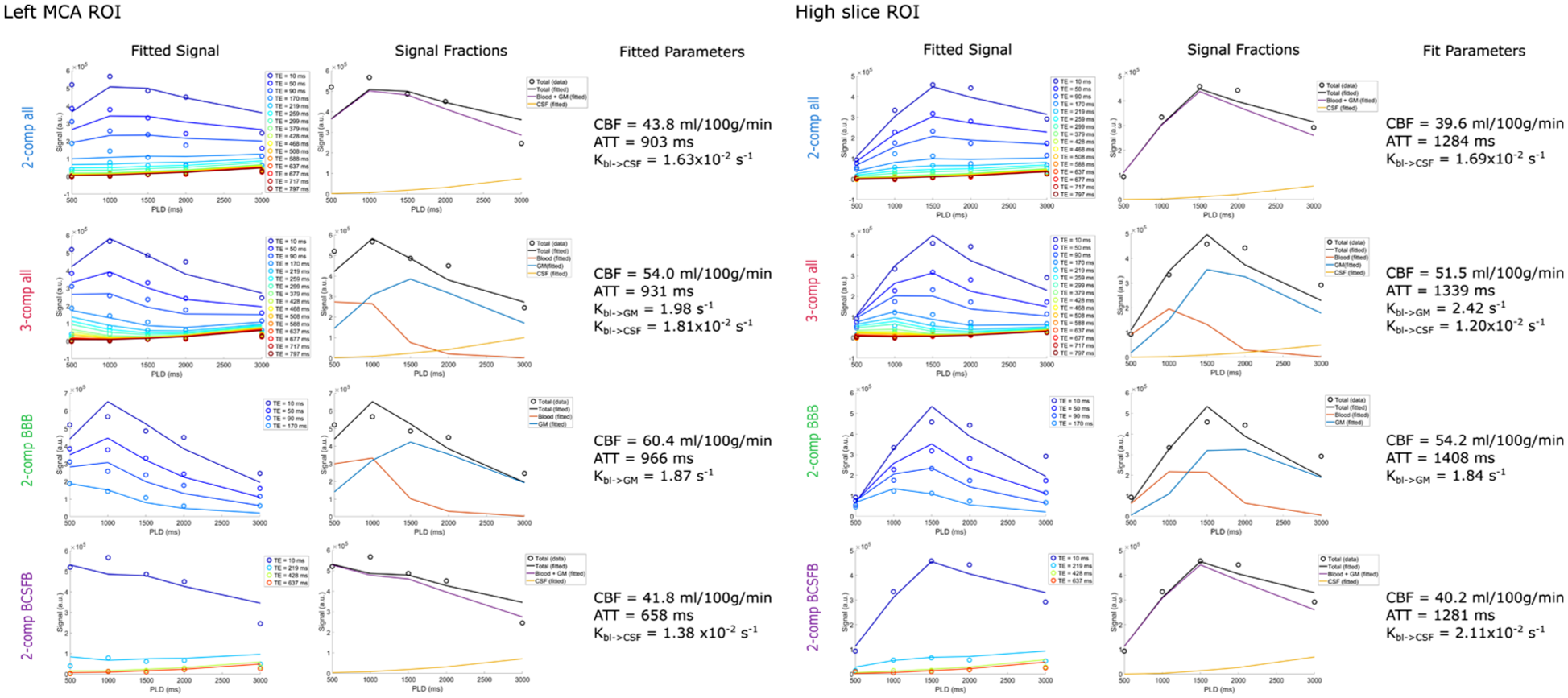
Model fitting of the signal in the left MCA territory ROI (single slice, containing 390 voxels) and the high slice ROI (single slice, containing 338 voxels) of subject 5 for all four models. The first column shows the signal (circles) and fitted curves (lines) for the different echo times. The second column shows the signal in each compartment based on the fit, and the third column shows the fitted parameters.

Parameter mapping: Whole brain, GM, WM, and CP ROIs

Parameter maps for a single slice created by all models (subject 5) are shown in Figure 4 (for full brain maps of two other subjects see Supplementary Figures S4 and S5). The CBF and ATT maps are consistent with literature. The CBF shows a typical perfusion pattern, while the ATT map highlights large arteries (the middle cerebral arteries and the anterior cerebral artery) and prolonged ATT in the posterior region of the brain and border zones. K_bl_→ GM is fairly uniform across the brain with notably lower values for the 2-comp BBB model. Finally, K_bl_→ CSF maps show contrast between the CP (situated at the center of this slice), with visibly higher values (because of the presence of the BCSFB) than the rest of the brain. Exchange rates are otherwise more or less homogenous across the GM, with more variations seen in the 3-comp all model, where regions with limited K_bl_→ CSF exchange appear especially in the WM and K_bl_→ GM is more homogenous throughout the brain.

Figure 4.

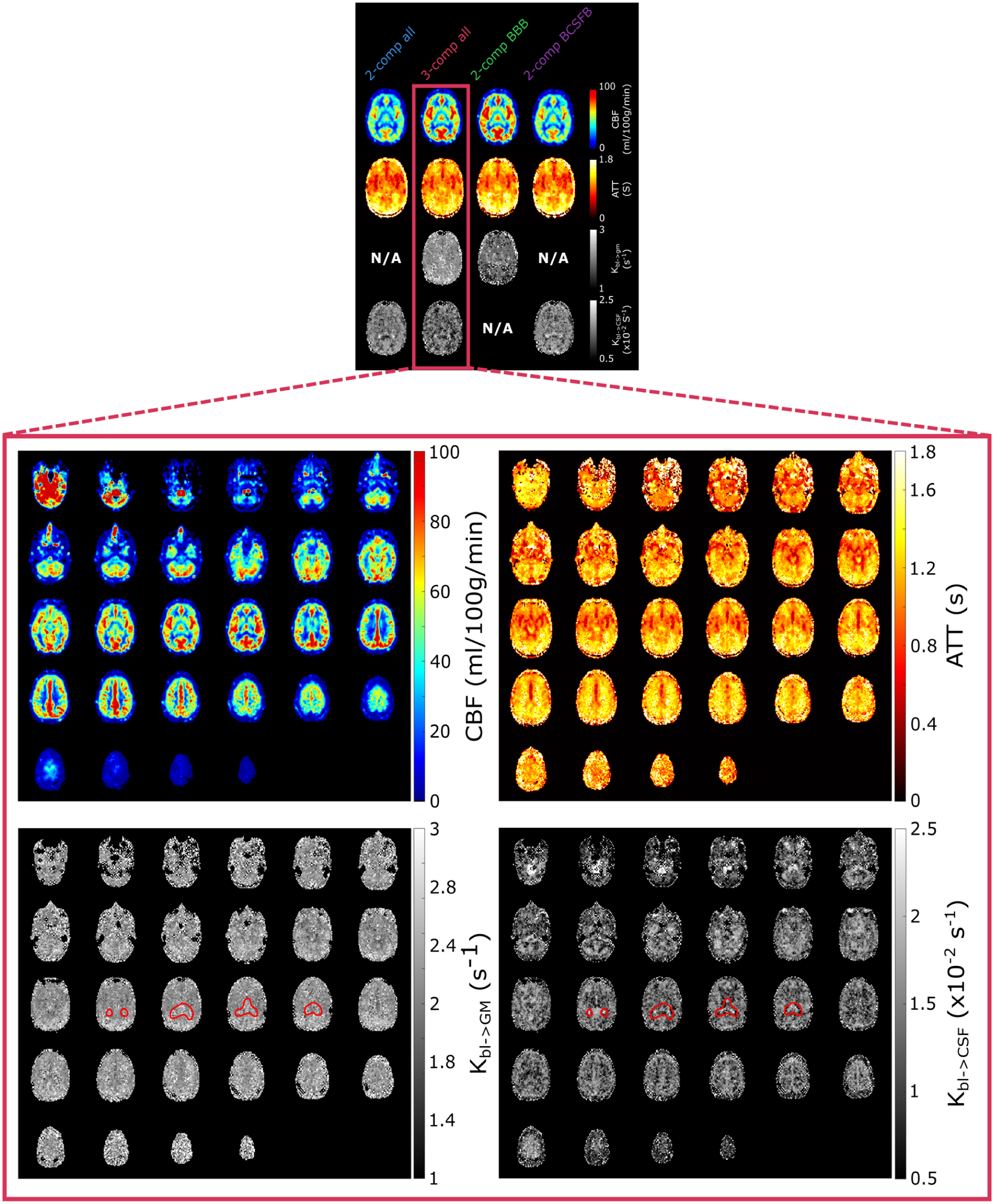
(Above) Single slice parameter maps for all models in subject 5. (Below) Whole-brain parameter maps in subject 5 for the 3-comp all model. The choroid plexus is circled in red. The first two and lowest slices of the brain (top left corner) intersect with the labeling plane, explaining the presence of high erroneous signal.

Whole-brain parameter maps are shown in Figure 4 for the 3-comp all model. Here the CP is encircled in red to highlight differences in K_bl_→ GM and K_bl_→ CSF in this region. The contrast between brain regions is more visible in the whole-brain maps and we can see how parameters vary across the entire brain. The CP in particular is clearly visible in the K_bl_→ CSF map with its elevated exchange values. There is also contrast between the gray and white matter, with slower exchange in the WM, and faster K_bl_→ CSF exchange in the higher slices where cortical GM and SAS are bordering. The K_bl_→ GM map shows less contrast, but appears to result in lower values around the large arteries (circle of Willis and ACA).

For a direct spatial comparison of these parameters across different tissue regions, the maps were averaged over the GM, SAS, CP, and WM ROIs. The averaged parameter values are shown in Figure 5 for all subjects and models. It is important to note that, although these ROIs were defined using tissue-specific masks and primarily represent regions dominated by the corresponding tissue types, they were not assumed to consist exclusively of a single tissue type. As a result, the ROIs are likely to include partial-volume contributions from surrounding tissues. For example, voxels within the GM ROI may contain partial-volume contributions from the SAS, such that at late TEs CSF signal is present within these voxels, allowing quantification of K_bl_→ CSF reflecting label exchange into this CSF compartment. CBF values are fairly consistent with literature, with the exception of the average GM CBF between 30 and 50 ml/100 g/min, which is lower than average.^46,47 The values in the CP around 35 ml/100 g/min⁴⁸ and in the WM around 20 ml/100 g/min⁴⁷ however are appropriate. For the ATT, values are also within the expected range, with longer transit times in the CP and WM as commonly observed in the literature. The tendency previously seen in ROI analyses and maps for the 2-comp BBB model to overestimate both CBF and ATT and for the 2-comp all and 2-comp BCSFB models to underestimate them compared to the 3-comp all model is clearly visible in these graphs. For K_bl_→ GM, differences between the models are far greater than differences between brain regions (~2 s^–1 for all regions using the 3-comp all model, ~1.4 s^–1 for the 2-comp BBB). Potential reasons for the low contrast in this parameter between brain regions will be addressed in the discussion. Finally, K_bl_→ CSF is approximately a factor 100 lower than K_bl_→ GM, with values ranging from ~1–1.4 × 10⁻² s^–1 in the WM ROI, to ~1.2–1.6 × 10^{−2 s^–1} in the GM and SAS ROIs, to ~1.5–2 × 10⁻² s^–1 in the CP. Here the contrast between brain regions is clear; there is fastest exchange in the CP, and the slowest exchange is seen in the WM.

Figure 5.

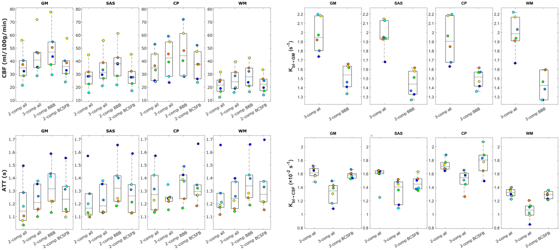
Average values of model parameters fitted with the four compartmental models for all subjects in GM, SAS, CP, and WM ROIs. Note that K_bl_→ GM is denoted referencing only GM rather than other extravascular tissue compartments that label may have exchanged into (such as WM) because during model fitting the assumed extravascular T₂ is that of GM.

Discussion

In this work, we aimed to simultaneously measure water exchange in the human brain from the blood to the GM and to the CSF. We also compared the CBF, ATT, and exchange parameters K_bl_→ GM and K_bl_→ CSF obtained by fitting four different compartmental models to our data. Our key takeaways are that our imaging protocol allows the measurement of ASL signal in the blood, GM, and CSF with its combination of LD/PLDs and echo times, and additionally that all compartmental models demonstrated comparable applicability to the data. Therefore, including the second exchange parameter in the 3-comp all model did not meaningfully improve or degrade the quality of the fit. Nevertheless, we believe that the 3-comp all model most accurately represents the underlying physiology since it provides information about the separate water exchange processes between the three tissue compartments where exchange is thought to occur during our measurements.

The combination of T_2prep and multi-echo readout was effective in measuring ASL signal for a large range of TEs with sufficient small inter-echo spacing. The ASL signal (Figure 1) is consistent with literature, and shows a relatively smooth transition from high signal in the short TEs to low signal in long TEs. The longest TEs (from ~500 ms) effectively isolate CSF signal as seen in the complete decay of blood and GM signal in the first two time points at longer TEs, followed by the gradual increase in long-TE signal consistent with the later arrival of labeled water in the CSF.

Furthermore, the proposed compartmental models provided good fits to the signal, with the 3-comp all model resulting in the most informative representation. Analyses of the left MCA and high slice ROIs (Figure 3) show this fit in detail for all TE and PLD data points. All models offered reasonable fits to the data, and resulted in distinct parameter values for these two ROIs. These differences reflect variations in compartment dynamics consistent with the differing tissue compositions of the ROIs (see Section 3.2 for details on the proportions of GM, WM, and CSF in each ROI). For example, the high slice was associated with longer ATTs, higher blood-to-CSF water exchange rate (because of the presence of more CSF) and lower blood-to-GM exchange. By visual inspection, the 3-comp all model showed the closest fit to the ROI data.

Turning to the brain-wide tissue region ROI analyses, the parameter maps shown in Figure 4 and the regional averages in Figure 5 demonstrate that the 3-comp all model provided good contrast in K_bl_→ CSF across brain regions, with faster exchange in the CP compared with the SAS, GM, and WM ROIs. This is consistent with the BCSFB at the CP being a known site of substantial water exchange.^49,50 The similar K_bl_→ CSF values observed in the SAS and GM ROIs indicate a more brain-wide phenomenon of water exchange from blood to CSF, in line with previous ASL studies.²⁸ The K_bl_→ CSF measurements in the GM ROI may be interpreted as reflecting label exchange from blood into CSF compartments (e.g. periarterial or subarachnoid spaces), or label that first enters parenchymal GM compartments and subsequently moves into CSF, for example, via periarterial or perivenous spaces. With respect to this latter pathway, it seems unlikely that ASL label exists long enough to fully resolve a blood → GM → CSF transport route. A rough estimate of the time required for a spin to freely diffuse from a penetrating arteriole to a perivascular space via the brain tissue—assuming a random walk distance of ~280 µm and a diffusion coefficient of D = 1.0 × 10⁻³ mm² s^–1 yields an approximate diffusion time of 13 s.^51–53 This timescale exceeds that of our ASL measurements, even for the longest LD/PLD pair (4/3 s). In addition, we expect T₁ decay of the label to be too rapid for any detectable signal to survive this pathway as label would experience the tissue T₁ for considerable time. considerable time. Consequently, we believe that the measured signal most likely reflects direct blood-to-CSF exchange, and the 3-comp all model is defined to represent this more probable route. This is, however, speculative and further studies would be valuable to determine whether a GM-mediated pathway could occur within the timescales of these measurements. Results for the K_bl_→ GM parameter, are more intuitive to interpret. The values for this parameter were more homogenous throughout the brain, and differences between averages in the four regions of the brain were negligible compared to the difference between the results of the 3-comp all and 2-comp BBB models. The 2-comp BBB model consistently yielded slower exchange (lower K_bl_→ GM) than the 3-comp all model, resulting in a higher fraction of signal in the blood compared to the 3-comp all model (see Figure 2).

Several studies using multi-echo and diffusion-prepared ASL report K_bl_→ GM values that closely match our 3-comp all model estimates (1.6–2.3 s^–1).^{1,31,32,54–56} Other studies report higher values (3.2–5 s^–1),^55,57–59 but these still align more closely with the 3-comp all model than with the 2-comp BBB model. A contrast-enhanced ASL study⁶⁰ likewise shows good agreement with the 3-comp all results. However, direct comparison across studies should be interpreted with caution. Aging effects,^55,57,58 differences in acquisition sequences, and variations in modeling and fitting procedures all introduce substantial variability, limiting the reliability of cross-study comparisons. In contrast, literature on K_bl_→ CSF is limited. The values of K_bl_→ CSF obtained here are consistent with those from our previous multi-echo study,²⁸ agreeing more closely with the 2-comp all model estimates which is expected given the previous work applied a two-compartment model. Other techniques applied in humans include REXI,⁶¹ which has reported substantially higher exchange rate in the CP, though direct comparison is inappropriate due to differing acquisition and modeling assumptions. Taso and Alsop’s T₂-prepared FLAIR approach⁶² indicates increased exchange in the CP, consistent with our findings, but does not yield a parameter directly comparable to K_bl_→ CSF. Several additional techniques have been proposed in animal models^63–65 but have not yet been translated to humans. A major limitation of the field—and of the present work—remains the lack of validated human reference standards for CSF water-exchange measurements.

In addition, variability in T₂ of arterial blood due to its dependency on oxygenation might have influenced the results.⁶⁶ The similarity in values between brain regions could likewise be due to limitations of the fitting technique, or could indicate that the phenomenon which we aim to characterize, that is, the exchange of water from blood to tissue, is present throughout the brain at a comparable rate. The models employ literature values of GM for all brain tissues, that is, also for WM. This can be justified by their relative similar T₂s compared to the much more different properties of CSF. Additionally, the 3-comp all model not only resulted in acceptable parameter values and good contrast between brain regions, but it also provided better separation of the signal originating from the three compartments (Figure 2), especially with less overlap between blood and GM compartments compared to the 2-comp BBB model. The remaining overlap between blood and GM could be due to the aforementioned variable blood T₂, or we may simply be observing the blood-to-GM water exchange occurring closer to the large vessels in early time points leading to the appearance of vascular signal in the GM compartment in the first two PLDs. In addition, the compartmental models used do not include a macrovascular compartment (i.e. blood contained in the large arteries instead of arterioles and capillaries), and may thus break down in the presence of large arteries. Finally, the addition of the third compartment might be considered more realistic on theoretical grounds, as blood, GM, and CSF are three distinct compartments with water exchange from the blood to the latter two occurring at appreciably different rates and governed by barriers with unique cellular components and transport mechanisms.

The AIC analysis didn’t favor a specific model as both models yielded similar AIC values across all brain regions, with the 2-comp all model exhibiting slightly lower AIC values. According to the literature, a difference in AIC (relative to the model with the lowest AIC value) in the range of 2–7 indicates a reasonable fit quality and thus that a model should not be disregarded.⁶⁷ On average, the AIC difference between the 2-comp all and 3-comp all models does not exceed 2, suggesting that both models can be considered as providing comparable quality fits to the data. This finding indicates that the additional fitting parameter (K_bl_→ GM) in the 3-comp all model does not lead to overfitting, a conclusion further supported by visual inspection of the fitted curves in Figure 3. Since both models demonstrate acceptable fit quality, we argue that for a similar level of error the 3-comp all model is superior because it more accurately represents the underlying physiology. Specifically, it distinguishes between blood and GM as distinct compartments, allowing the two exchange parameters (K_bl_→ GM and K_bl_→ CSF) to be extracted from a single sequence and fitting procedure, thus offering a more comprehensive view of brain water exchange dynamics.

There are a number of limitations to this study which should be noted. Firstly, the imaging sequences used are long, and a lot of optimization was needed to reach a satisfactory range of echo times and LD/PLDs which would fit into an hour of scanning. The timing was so limiting that the T₁w image that would usually be acquired with such a protocol had to be forgone. A T₁w scan is typically used to create GM, WM, and CSF masks which can subsequently be coregistered to the ASL data, but here we had to use more indirect masking techniques which may have resulted in less effective separation of tissue types. This might also explain the fact that the GM CBF values were lower in this study than typically observed in literature. The long scan times limit the clinical translatability of this method for which it may be more efficient to employ Hadamard time-encoding for BBB characterization, along with separate longer LD/PLD and TE T₂-prepared acquisitions as implemented in this paper for the BCSFB. Reducing the number of sampled TEs and/or PLDs could also be beneficial however extensive simulations, such as leave-one-out cross-validation, would be required to ensure model sensitivity to exchange time and hemodynamic parameters is maintained.

Secondly, the ASL signal did show some instability through the TEs, with some small increases appearing at longer TEs. This is also observed when averaging signal over ROIs and plotting over TEs (shown in Supplementary Figure S6 for the two ROIs), where a slight saw-tooth effect was present. We however found that these variations were small in comparison to the natural signal decay along TEs, but these could still induce some errors in the analysis of this signal. This pattern could be caused simply by the interleaved nature of the acquisition of TEs with natural fluctuations in perfusion and physiological processes over the long scan time, or it could arise from an interaction between the T_2prep module and the readout module (and BGS). However, this behavior was different in different subjects (i.e. signal peaks did not occur at the same TEs). These variations were deemed acceptable in the context of this work, but further improvements in sequence design could alleviate this issue, for example, by limiting the overall temporal footprint.

Additionally, these data are of course acquired in a small cohort of healthy individuals, and it therefore did not have statistical power to study the relationship between water exchange rates and, for example, age and sex. Testing this technique in larger groups of subjects as well as in patient populations is critical to reach a better understanding of the role of brain water exchange in health, aging, and disease.

Finally, the most relevant limitation of this work is the absence of a reliable reference standard for validating water-exchange measurements. As a result, particularly for K_bl_→ CSF which is a novel exchange parameter, some analyses remain qualitative or speculative. Validation will require comparison with techniques that probe the same mechanisms of water transport across the BBB and BCSFB. Existing MRI measures of BBB function, such as DCE-MRI, are not directly comparable to water-exchange metrics: gadolinium transport rate reflects function of different BBB mechanisms and studies measuring both modalities show that the two measures can be related but not in a one-to-one manner, with correlations present in some regions or cohorts but absent in others.^68–71 Although H₂¹⁵O PET uses water as a tracer, and is the reference method for in-vivo BBB water permeability, it lacks the ability of MRI to differentiate compartments on compartment specific parameters such as the T₂ and also employs different kinetic modeling, making the measures non-equivalent.⁷² H₂¹⁷O MRI⁷³ is an avenue that shows promise in regard to BCSFB characterization, although its translation to the human brain may be difficult because of its prohibitive cost.

In conclusion, we find that the combination of a T_2prep module with a multi-echo 3D GRASE readout allows the non-invasive measurement of ASL signal at a wide range of echo times necessary for the simultaneous characterization of the BBB and the BCSFB. The proposed compartmental models were effective in measuring perfusion and exchange parameters, and in particular the three-compartment model showed promise to provide a more complete picture of the dynamics of water exchange between blood, GM, and CSF.

Supplemental Material

sj-docx-1-jcb-10.1177_0271678X261429042 – Supplemental material for Simultaneous measurement of water transport across the blood–brain and blood–CSF barrier in the human brain with arterial spin labeling MRI

Supplemental material, sj-docx-1-jcb-10.1177_0271678X261429042 for Simultaneous measurement of water transport across the blood–brain and blood–CSF barrier in the human brain with arterial spin labeling MRI by Léonie Petitclerc, Helena Durrant, Lydiane Hirschler, Lena Václavů and Matthias J.P. van Osch in Journal of Cerebral Blood Flow & Metabolism

Footnotes

Acknowledgements

The authors thank Prof. Dr. Jelle J Goeman for statistical advice regarding Akaike Information Criterion analysis.

Abbreviations

ASL = Arterial spin labeling

AIC = Akaike information criterion

AP = Anterior-to-posterior

ATT = Arterial transit time

BBB = Blood–brain barrier

BCSFB = Blood–CSF barrier

BGS = Background suppression

CBF = Cerebral blood flow

CP = Choroid plexus

CSF = Cerebrospinal fluid

eTE = Effective echo time

GM = Gray matter

Gd = Gadolinium

GRASE = Gradient and spin-echo

ISF = Interstitial fluid

K_bl_→ GM = Exchange rate from blood to GM

K_bl_→ CSF = Exchange rate from blood to CSF

LD = Labeling duration

PCASL = Pseudo-continuous arterial spin labeling

PLD = Post-labeling delay

PVS = Perivascular space

RL = Right-to-left

SAS = Subarachnoid space

T_2prep = T₂ preparation module

TE = Echo time

TR = Repetition time

WM = White matter

Author contributions

Léonie Petitclerc: conceptualization, methodology, software, formal analysis, data curation, writing, visualization. Helena Durrant: software, formal analysis, data curation, writing, visualization. Lydiane Hirschler: conceptualization, methodology, writing. Lena Václavů: investigation, software, writing, supervision. Matthias J.P. van Osch: conceptualization, methodology, writing, supervision, funding acquisition.

Funding

The authors disclosed receipt of the following financial support for the research, authorship, and/or publication of this article: This work is part of the research programme Innovational Research Incentives Scheme Vici with project number 016.160.351, which is financed by the Netherlands Organisation for Scientific Research. Lena Václavů is supported by the Dutch Research Council (NWO) Talent Programme Veni (Project No. 20212), which is partly financed by the NWO. Helena Durrant, Matthias J.P. van Osch, and Lena Václavů received funding from MODEM, a Dutch national consortium part of the Dementia Research Program of ZonMw (grant #10510032120006) supported by the National Dementia Strategy 2021–2030 of the Dutch Ministry of Health, Welfare, and Sport. Helena Durrant received funding from Alzheimer Nederland (#WE.30-2022-04) supporting MODEM research. Matthias J.P. van Osch and Lydiane Hirschler received support from a grant from the Leducq Foundation and the Leducq Foundation for Cardiovascular Research (23CVD03) and from the Joint Program for Neurodegenerative Diseases on Human Brain Clearance Imaging.

Declaration of conflicting interests

The authors declared the following potential conflicts of interest with respect to the research, authorship, and/or publication of this article: The research groups of Matthias J.P. van Osch and Lena Václavů receive research support from Philips.

Ethical considerations

This research was carried out in accordance with our institution’s IRB regulations (Medisch Etische Toetsingscommissie (METC), Leiden–Den Haag–Delft) and the Declaration of Helsinki.

Consent to participate

All participants gave written informed consent prior to participation.

Consent for publication

All participants gave written informed consent for non-identifiable images to be used for publication.

ORCID iDs

Helena Durrant

Lydiane Hirschler

Lena Václavů

Matthias J.P. van Osch

Data availability statement

Due to the restrictions of the informed consent, the data is not available publicly, but can be provided upon reasonable request to the corresponding or last author.

Supplemental material

Supplemental material for this article is available online.

References

Dickie

Parker

Parkes

LM.

Measuring water exchange across the blood–brain barrier using MRI. Prog Nucl Magn Reson Spectrosc 2020; 116: 19–39.

Paulson

Blood–brain barrier, brain metabolism and cerebral blood flow. Eur Neuropsychopharmacol 2002; 12: 495–501.

Weiss

Miller

Cazaubon

, et al. The blood–brain barrier in brain homeostasis and neurological diseases. Biochim Biophys Acta 2009; 1788: 842–857.

Zlokovic

BV.

The blood–brain barrier in health and chronic neurodegenerative disorders. Neuron 2008; 57: 178–201.

Nedergaard

Goldman

SA.

Glymphatic failure as a final common pathway to dementia. Science 2020; 370: 50–56.

Obermeier

Daneman

Ransohoff

RM.

Development, maintenance and disruption of the blood–brain barrier. Nature medicine 2013; 19: 1584–1596.

Raja

Rosenberg

Caprihan

MRI measurements of blood–brain barrier function in dementia: a review of recent studies. Neuropharmacology 2018; 134: 259–271.

Staals

Booth

Morris

, et al. Total MRI load of cerebral small vessel disease and cognitive ability in older people. Neurobiol Aging 2015; 36: 2806–2811.

Starr

Farrall

Armitage

, et al. Blood–brain barrier permeability in Alzheimer’s disease: a case–control MRI study. Psychiatry Res 2009; 171: 232–241.

10.

Tarasoff-Conway

Carare

Osorio

, et al. Clearance systems in the brain—implications for Alzheimer disease. Nat Rev Neurol 2015; 11: 457–470.

11.

Wardlaw

Benveniste

Nedergaard

, et al. Perivascular spaces in the brain: anatomy, physiology and pathology. Nat Rev Neurol 2020; 16: 137–153.

12.

Zenaro

Piacentino

Constantin

The blood–brain barrier in Alzheimer’s disease. Neurobiol Dis 2017; 107: 41–56.

13.

Heye

Culling

Hernández

MdCV

, et al. Assessment of blood–brain barrier disruption using dynamic contrast-enhanced MRI. A systematic review. Neuroimage Clin 2014; 6: 262–274.

14.

Eide

Mariussen

Uggerud

, et al. Clinical application of intrathecal gadobutrol for assessment of cerebrospinal fluid tracer clearance to blood. JCI Insight 2021; 6: e147063.

15.

Ringstad

Eide

PK.

Cerebrospinal fluid tracer efflux to parasagittal dura in humans. Nat Commun 2020; 11: 354.

16.

Gulani

Calamante

Shellock

, et al. Gadolinium deposition in the brain: summary of evidence and recommendations. Lancet Neurol 2017; 16: 564–570.

17.

Fischer

Gottschlich

Seelig

Blood–brain barrier permeation: molecular parameters governing passive diffusion. J Membr Biol 1998; 165: 201–211.

18.

Nitta

Hata

Gotoh

, et al. Size-selective loosening of the blood–brain barrier in claudin-5-deficient mice. J Cell Biol 2003; 161: 653–660.

19.

Armitage

Farrall

Carpenter

, et al. Use of dynamic contrast-enhanced MRI to measure subtle blood–brain barrier abnormalities. Magn Reson Imaging 2011; 29: 305–314.

20.

Cramer

Larsson

HB.

Accurate determination of blood–brain barrier permeability using dynamic contrast-enhanced T₁-weighted MRI: a simulation and in vivo study on healthy subjects and multiple sclerosis patients. J Cereb Blood Flow Metab 2014; 34: 1655–1665.

21.

Cramer

Simonsen

Frederiksen

, et al. Abnormal blood–brain barrier permeability in normal appearing white matter in multiple sclerosis investigated by MRI. Neuroimage Clin 2014; 4: 182–189.

22.

Montagne

Barnes

Sweeney

, et al. Blood–brain barrier breakdown in the aging human hippocampus. Neuron 2015; 85: 296–302.

23.

Taheri

Gasparovic

Huisa

, et al. Blood–brain barrier permeability abnormalities in vascular cognitive impairment. Stroke 2011; 42: 2158–2163.

24.

van de Haar

Burgmans

Hofman

, et al. Blood–brain barrier impairment in dementia: current and future in vivo assessments. Neurosci Biobehav Rev 2015; 49: 71–81.

25.

Van De Haar

Burgmans

Jansen

, et al. Blood–brain barrier leakage in patients with early Alzheimer disease. Radiology 2016; 281: 527–535.

26.

Evans

Sokolska

Alves

, et al. Non-invasive MRI of blood–cerebrospinal fluid barrier function. Nat Commun 2020; 11: 2081.

27.

Liu

Determination of spin compartment in arterial spin labeling MRI. Magn Reson Med 2011; 65: 120–127.

28.

Petitclerc

Hirschler

Wells

, et al. Ultra-long-TE arterial spin labeling reveals rapid and brain-wide blood-to-CSF water transport in humans. Neuroimage 2021; 245: 118755.

29.

Petitclerc

Schmid

Hirschler

, et al. Combining T₂ measurements and crusher gradients into a single ASL sequence for comparison of the measurement of water transport across the blood–brain barrier. Magn Reson Med 2021; 85: 2649–2660.

30.

Shao

Casey

, et al. Mapping water exchange across the blood–brain barrier using 3D diffusion-prepared arterial spin labeled perfusion MRI. Magn Reson Med 2019; 81: 3065–3079.

31.

St. Lawrence

Owen

Wang

DJ.

A two-stage approach for measuring vascular water exchange and arterial transit time by diffusion-weighted perfusion MRI. Magn Reson Med 2012; 67: 1275–1284.

32.

Gregori

Schuff

Kern

, et al. T₂-based arterial spin labeling measurements of blood to tissue water transfer in human brain. J Magn Reson Imaging 2013; 37: 332–342.

33.

Grgac

, et al. Calibration and validation of TRUST MRI for the estimation of cerebral blood oxygenation. Magn Reson Med 2012; 67: 42–49.

34.

Schmid

Teeuwisse

, et al. Time-efficient determination of spin compartments by time-encoded pCASL T₂-relaxation-under-spin-tagging and its application in hemodynamic characterization of the cerebral border zones. Neuroimage 2015; 123: 72–79.

35.

Spijkerman

Petersen

Hendrikse

, et al. T 2 mapping of cerebrospinal fluid: 3 T versus 7 T. Magn Reson Mater Phys Biol Med 2018; 31: 415–424.

36.

Stanisz

Odrobina

Pun

, et al. T₁, T₂ relaxation and magnetization transfer in tissue at 3T. Magn Reson Med 2005; 54: 507–512.

37.

Wansapura

Holland

Dunn

, et al. NMR relaxation times in the human brain at 3.0 tesla. J Magn Reson Imaging 1999; 9: 531–538.

38.

Zhang

Petersen

Ghariq

, et al. In vivo blood T₁ measurements at 1.5 T, 3 T, and 7 T. Magn Reson Med 2013; 70: 1082–1086.

39.

Hopkins

Yeung

Bratton

Multiple field strength in vivo T₁ and T₂ for cerebrospinal fluid protons. Magn Reson Med 1986; 3: 303–311.

40.

Chen

Zhang

Yuan

, et al. Measuring the labeling efficiency of pseudocontinuous arterial spin labeling. Magn Reson Med 2017; 77: 1841–1852.

41.

Garcia

Duhamel

Alsop

DC.

Efficiency of inversion pulses for background suppressed arterial spin labeling. Magn Reson Med 2005; 54: 366–372.

42.

Herscovitch

Raichle

ME.

What is the correct value for the brain–blood partition coefficient for water?. J Cereb Blood Flow Metab 1985; 5: 65–69.

43.

Akaike

Akaike’s information criterion. In: Lovric

(ed.) International encyclopedia of statistical science. Berlin/Heidelberg: Springer, 2011, pp.25–25.

44.

Heye

Thrippleton

Armitage

, et al. Tracer kinetic modelling for DCE–MRI quantification of subtle blood–brain barrier permeability. Neuroimage 2016; 125: 446–455.

45.

Burnham

Anderson

DR.

Model selection and multimodel inference: a practical information-theoretic approach. New York, NY: Springer, 2002.

46.

Buxton

RB.

Quantifying CBF with arterial spin labeling. J Magn Reson Imaging 2005; 22: 723–726.

47.

Parkes

Rashid

Chard

, et al. Normal cerebral perfusion measurements using arterial spin labeling: reproducibility, stability, and age and gender effects. Magn Reson Med 2004; 51: 736–743.

48.

Alisch

Kiely

Triebswetter

, et al. Characterization of age-related differences in the human choroid plexus volume, microstructural integrity, and blood perfusion using multiparameter magnetic resonance imaging. Front Aging Neurosci 2021; 13: 734992.

49.

MacAulay

Keep

Zeuthen

Cerebrospinal fluid production by the choroid plexus: a century of barrier research revisited. Fluids Barriers CNS 2022; 19: 26.

50.

Lun

Monuki

Lehtinen

MK.

Development and functions of the choroid plexus–cerebrospinal fluid system. Nat Rev Neurosci 2015; 16: 445–457.

51.

Adams

Piserchia

Economides

, et al. Vascular supply of the cerebral cortex is specialized for cell layers but not columns. Cereb Cortex 2015; 25: 3673–3681.

52.

Dietrich

Biffar

Baur-Melnyk

, et al. Technical aspects of MR diffusion imaging of the body. Eur J Radiol 2010; 76: 314–322.

53.

Duvernoy

Delon

Vannson

Cortical blood vessels of the human brain. Brain Res Bull 1981; 7: 519–579.

54.

Gold

Shao

Sudduth

, et al. Water exchange rate across the blood–brain barrier is associated with CSF amyloid-β 42 in healthy older adults. Alzheimers Dement 2021; 17: 2020–2029.

55.

Morgan

Thomas

Shao

, et al. Measurement of blood–brain barrier water exchange rate using diffusion-prepared and multi-echo arterial spin labelling: comparison of quantitative values and age dependence. NMR Biomed 2024; 37: e5256.

56.

Shao

Zhao

Shou

, et al. Quantification of blood–brain barrier water exchange and permeability with multidelay diffusion-weighted pseudo-continuous arterial spin labeling. Magn Reson Med 2023; 89: 1990–2004.

57.

Mahroo

Konstandin

Günther

Blood–brain barrier permeability to water measured using multiple echo time arterial spin labeling MRI in the aging human brain. J Magn Reson Imaging 2024; 59: 1269–1282.

58.

Padrela

Slivka

Sneve

, et al. Blood–brain barrier water permeability across the adult lifespan: a multi-echo ASL study. Neurobiol Aging 2025; 147: 176–186.

59.

Wang

Fernández-Seara

Wang

, et al. When perfusion meets diffusion: in vivo measurement of water permeability in human brain. J Cereb Blood Flow Metab 2007; 27: 839–849.

60.

Powell

Dickie

Ohene

, et al. Blood–brain barrier water exchange measurements using contrast-enhanced ASL. NMR Biomed 2023; 36: e5009.

61.

Tan

Zhang

, et al. Feasibility of relaxation-exchange magnetic resonance imaging (REXI) for measuring water exchange across the blood–CSF barrier in the human choroid plexus. J Cereb Blood Flow Metab 2025; 46: 508–520.

62.

Taso

Alsop

DC.

Tissue-to-fluid water-exchange imaging using T₂-selective saturation labeling. Magn Reson Med 2025; 94: 150–165.

63.

Chen

Lai

, et al. The effect of aquaporin-4 inhibition on cerebrospinal fluid-tissue water exchange in mouse brain detected by magnetization transfer indirect spin labeling MRI. NMR Biomed 2024; 37: e5093.

64.

Chen

Liu

, et al. Age-dependent cerebrospinal fluid–tissue water exchange detected by magnetization transfer indirect spin labeling MRI. Magn Reson Med 2022; 87: 2287–2298.

65.

Cerebrospinal fluid–tissue exchange revealed by phase alternate labeling with null recovery MRI. Magn Reson Med 2022; 87: 1207–1217.

66.

Chen

Pike

GB.

Human whole blood T₂ relaxometry at 3 Tesla. Magn Reson Med 2009; 61: 249–254.

67.

Burnham

Anderson

Huyvaert

KP.

AIC model selection and multimodel inference in behavioral ecology: some background, observations, and comparisons. Behav Ecol Sociobiol 2011; 65: 23–35.

68.

Dickie

Boutin

Parker

, et al. Alzheimer’s disease pathology is associated with earlier alterations to blood–brain barrier water permeability compared with healthy ageing in TgF344-AD rats. NMR Biomed 2021; 34: e4510.

69.

Shao

Jann

, et al. Comparison between blood–brain barrier water exchange rate and permeability to gadolinium-based contrast agent in an elderly cohort. Front Neurosci 2020; 14: 571480.

70.

Tiwari

Shen

, et al. Magnetic resonance imaging of blood–brain barrier permeability in ischemic stroke using diffusion-weighted arterial spin labeling in rats. J Cereb Blood Flow Metab 2017; 37: 2706–2715.

71.

Ying

Yao

, et al. Heterogeneous blood–brain barrier dysfunction in cerebral small vessel diseases. Alzheimers Dement 2024; 20: 4527–4539.

72.

Herscovitch

Raichle

Kilbourn

, et al. Positron emission tomographic measurement of cerebral blood flow and permeability—surface area product of water using [¹⁵O] water and [¹¹C] butanol. J Cereb Blood Flow Metab 1987; 7: 527–542.

73.

Alshuhri

Gallagher

Work

, et al. Direct imaging of glymphatic transport using H₂¹⁷O MRI. JCI Insight 2021; 6: e141159.