Sage Journals: Discover world-class research

Abstract

Despite extensive efforts to identify interhemispheric functional connectivity (FC) with resting-state (rs-) fMRI, correlated low-frequency rs-fMRI signal fluctuation across homotopic cortices originates from multiple sources. It remains challenging to differentiate circuit-specific FC from global regulation. Here, we developed a bilateral line-scanning fMRI method to detect laminar-specific rs-fMRI signals from homologous forepaw somatosensory cortices with high spatial and temporal resolution in rat brains. Based on spectral coherence analysis, two distinct bilateral fluctuation spectral features were identified: ultra-slow fluctuation (<0.04 Hz) across all cortical laminae versus Layer (L) 2/3-specific evoked BOLD at 0.05 Hz based on 4 s on/16 s off block design and resting-state fluctuations at 0.08–0.1 Hz. Based on the measurements of evoked BOLD signal at corpus callosum (CC), this L2/3-specific 0.05 Hz signal is likely associated with neuronal circuit-specific activity driven by the callosal projection, which dampened ultra-slow oscillation less than 0.04 Hz. Also, the rs-fMRI power variability clustering analysis showed that the appearance of L2/3-specific 0.08–0.1 Hz signal fluctuation is independent of the ultra-slow oscillation across different trials. Thus, distinct laminar-specific bilateral FC patterns at different frequency ranges can be identified by the bilateral line-scanning fMRI method.

Keywords

Callosal projection functional connectivity global neuromodulation high-resolution fMRI laminar specificity

Introduction

Resting-state (rs-) fMRI, as a non-invasive neuroimaging method, detects functional connectivity (FC) by measuring fMRI signal fluctuations during rest.^1–6 The fMRI signal oscillates at a low-frequency range less than 0.1 Hz, representing strong correlation among functional modules, e.g., symmetric cortices of two hemispheres.^7–9 Corpus callosum (CC), as major fibers connecting homologous cortical areas of two hemispheres, is considered to mediate bilateral FC.^8,10 Previously, significantly diminished bilateral FC has been reported in acallosal human brains^11–14 and post-callosotomy rodents.^15–17 Meanwhile, several reports have demonstrated nearly intact interhemispheric FC in individuals with callosotomy.^18–21 Also, both bilateral EEG human study²² and a non-human primate rs-fMRI study²³ demonstrate that after complete callosotomy the bilateral FC is reduced but exist, attributing to the brain network coordination via subcortical mechanism such as thalamocortical projection,^24–26 and other mechanism regulating arousal.²⁷ In recent studies, emerging evidence has shown that subcortical neuromodulatory projections mediate brain state changes, contributing to global and region-specific fMRI signal fluctuations.^28–38 Given unilateral visual stimuli, bilateral cortical activities was synchronized in voltage-sensitive dye imaging either under anesthesia or in awake condition,³⁹ showing that interhemispheric FC exists on a background of spontaneous activity.^40,41 Also, by genetically encoded Ca²⁺ indicator (GCaMP)-based recording of the Ca²⁺ signal fluctuation across two hemispheres, the bilateral global neuronal oscillatory signal at the low frequency can be regulated by the evoked neuronal signals, presenting a more complex regulatory mechanism underlying interhemispheric FC detected by rs-fMRI.⁴²

High field fMRI reveals laminar-specific responses to either bottom-up or top-down tasks, indicating neuronal circuit-based laminar specificity in human^43–47 and animal brains.^48–53 In contrast, the laminar-specific fMRI signal correlation/coherence patterns, which can illustrate underlying neuronal circuits for FC, have not been thoroughly investigated using conventional fMRI methods given the limited spatiotemporal resolution. Yu et al. have developed a line-scanning fMRI method to substantially improve spatial (50 μm) and temporal (50 ms) resolution with a line profile across different cortical layers in rat brains.⁵⁰ The ultra-fast sampling scheme of this method avoids the aliasing of the cardiorespiratory cycles over low-frequency fluctuation of rs-fMRI signals. Whereas, most slow sampling methods need retrospective correction for human brain mapping^54–60 and aliasing effect remains a challenging issue for rodent fMRI.^61–65 Meanwhile, the ultra-high spatial resolution provides a unique advantage to map distinct laminar BOLD signals with peripheral or optogenetic stimulation across the 1–2 mm rodent cortex.^50,51,53 Given the thickness of gray matter of human brains is in the comparable scale of the rodent cortex ranging from 1–4 mm,⁶⁶ the line-scanning fMRI enables the detailed layer-specific analysis of fMRI signals. Recently, both line-scanning BOLD and diffusion cortical mapping has been implemented to investigate layer-specific anatomical and evoked hemodynamic features in human brains.^46,67–70 Also, a recent animal fMRI study co-registered the brain-wide rs-fMRI correlation pattern and 3D Allen mouse brain atlas, presenting axonal tracing-based layer-specific neuronal connections underlying the default mode network.^9,71 To date, no direct measurement of laminar fMRI signals has been performed on symmetric cortices of two hemispheres to differentiate circuit-specific regulatory sources with high spatiotemporal resolution.

To study laminar-specific intrahemispheric FC, we developed a multi-slice line-scanning fMRI method to detect evoked and rs-fMRI signals from multiple line profiles with ultra-high spatiotemporal resolution.⁷² Here, a bilateral line-scanning fMRI (BiLS) method was used to record laminar fMRI signals in bilateral forepaw somatosensory cortex (FP-S1) and CC of anesthetized rats. In both evoked and resting states, we detected ultra-slow oscillation (<0.04 Hz) across all cortical layers, which can be directly differentiated from callosal circuit-specific bilateral coherent oscillation at Layer (L) 2/3, where callosal projection neurons are mainly located.^73,74 For experiments with electrical forepaw stimulation (20 s per epoch with 4 s on and 16 s off), the coherent frequency of bilateral BOLD signals was detected at 0.05 Hz, but during rest, the coherent frequency of bilateral rs-fMRI signal fluctuation was detected at 0.08–0.1 Hz. Noteworthily, the ultra-slow oscillation is significantly dampened upon stimulation, but L2/3-specific fMRI signal fluctuation (0.05 Hz due to periodic stimulation or 0.08–0.1 Hz during rest) is independent of the ultra-slow oscillation based on trial-specific analysis. Our findings demonstrate that the BiLS method enables the decomposition of frequency-specific interhemispheric low-frequency fluctuations, revealing two independent laminar-specific coherent bandwidths (i.e., 0.01–0.04 Hz versus 0.05 Hz for evoked fMRI or 0.08–0.1 Hz for rs-fMRI) presumably driven by different neuronal sources.

Materials and methods

Animal preparation

The study was performed in accordance with the German Animal Welfare Act (TierSchG) and Animal Welfare Laboratory Animal Ordinance (TierSchVersV). This is in full compliance with the guidelines of the EU Directive on the protection of animals used for scientific purposes (2010/63/EU). The study was reviewed by the ethics commission (§15 TierSchG) and approved by the state authority (Regierungspräsidium, Tübingen, Baden-Württemberg, Germany). A 12-12 hour on/off lighting cycle was maintained to assure undisturbed circadian rhythm. Food and water were available ad libitum. A total of 6 male Sprague–Dawley rats (4 weeks-old) were used in this study. The animal data reporting of the current study has followed the ARRIVE 2.0 guidelines with the reference (PMID: 32663096).

Anesthesia was first induced in the animal with 5% isoflurane in the chamber. The anesthetized rat was intubated using a tracheal tube and a mechanical ventilator (SAR-830, CWE, USA) was used to ventilate animals throughout the whole experiment. Femoral arterial and venous catheterization was performed with polyethylene tubing for blood sampling, drug administration, and constant blood pressure measurements. After the surgery, isoflurane was switched off, and a bolus of the anesthetic alpha-chloralose (80 mg/kg) was infused intravenously. After the animal was transferred to the MRI scanner, a mixture of alpha-chloralose (26.5 mg/kg/h) and pancuronium (2 mg/kg/h) was constantly infused to maintain the anesthesia and reduce motion artifacts.

EPI fMRI acquisition

All datasets from rats were acquired using a 14.1T/26 cm (Magnex, Oxford) horizontal bore magnet with an Avance III console (Bruker, Ettlingen) and a 12 cm diameter gradient system (100 G/cm, 150 µs rising time). A home-made transceiver surface coil with a 22 mm diameter was used on the rat brain in all experiments. For the functional map of BOLD activation (Figure 1(a), left), a 3D gradient-echo (GRE) EPI sequence was acquired with the following parameters: TR/TE 1500/11.5 ms, field of view (FOV) 1.92 × 1.92 × 1.92 cm³, matrix size 48 × 48 × 48, spatial resolution 0.4 × 0.4 ×0.4 mm³. A high order (e.g., 2nd or 3rd order) shimming was applied to reduce the main magnetic field (B0) inhomogeneities at the region-of-interest. For anatomical reference of the activated BOLD map, a RARE sequence was applied to acquire 48 coronal images with the same geometry as that of the EPI images. The fMRI design paradigm for each trial comprised 200 dummy scans to reach steady-state, 10 pre-stimulation scans, 3 scans during stimulation, and 12 post-stimulation scans with a total of 8 epochs.

Figure 1.

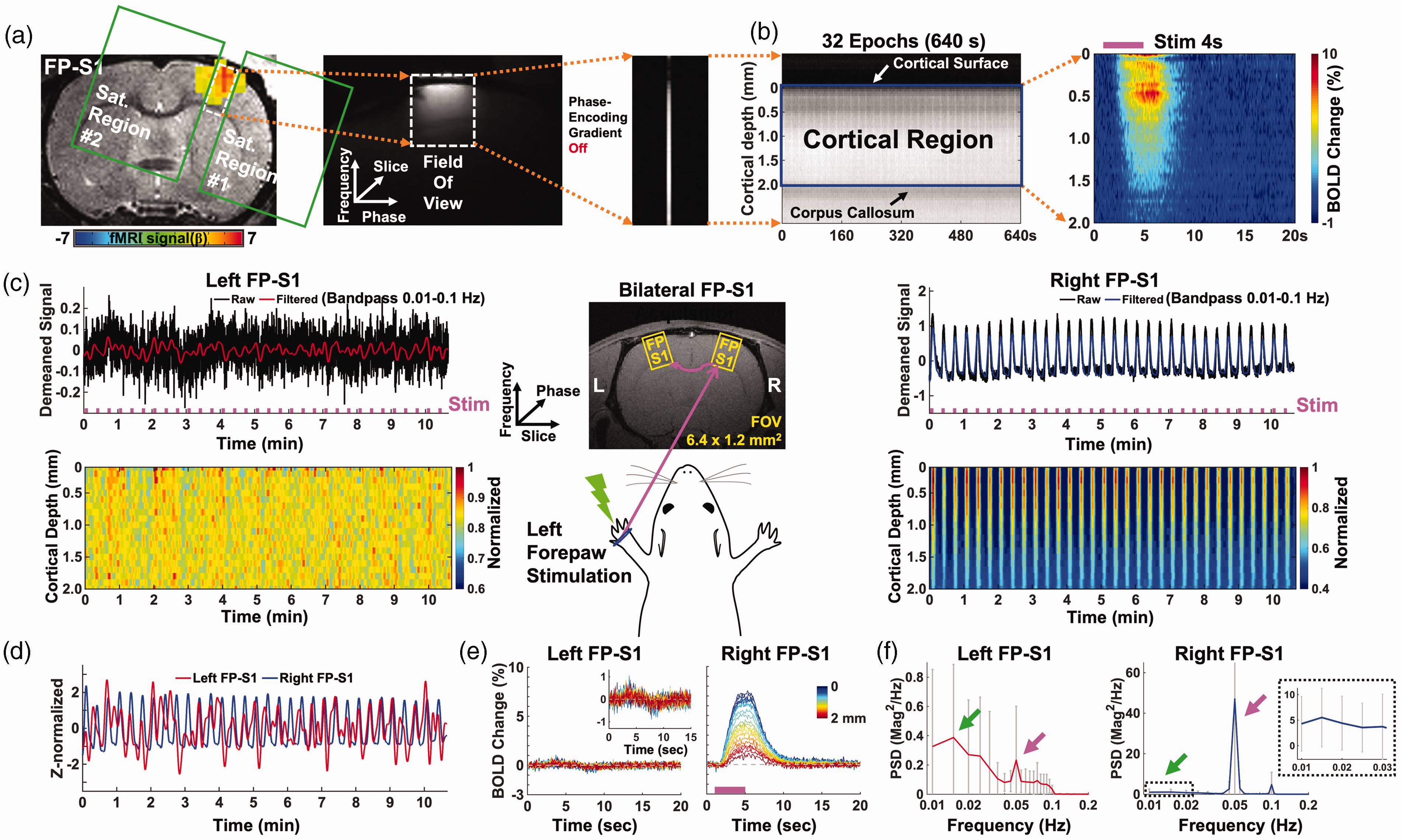
Evoked BOLD responses upon left forepaw stimulation using the unilateral and bilateral line-scanning method. (a–b) Sequential procedure to acquire the average BOLD change map in the unilateral line-scanning acquisition. (a) The procedure to set up the line-scanning method. Left: EPI BOLD activation map of forepaw somatosensory cortex overlaid on an anatomical RARE image. GLM-based t-statistics in AFNI is used, p < 0.001. Middle: Representative reduced FOV (6.4 × 1.2 mm²) image with 2 saturation slices. Right: Single line-scanning profile acquired without phase-encoding gradient. (b) Left: Spatiotemporal map concatenated with multiple line-scanning profiles for 32 epochs (10 min 40 sec). Right: Average BOLD percentage changes (block design: 1 s pre-stim, 4 s stim on and 15 s post-stim) show the laminar-specific BOLD responses across the cortical depth (0–2 mm, 50 μm resolution) from the cortical surface (white arrow) to the surface of the corpus callosum (black arrow). (c–f) Group-averaged results in bilateral line-scanning acquisition (n = 34 trials of 6 rats). (c) Top-left and-right: Demeaned fMRI time series (32 epochs, 10 min 40 sec) of raw (black) and filtered (red and blue) data (average of 20 voxels, bandpass: 0.01–0.1 Hz) in the left and right FP-S1 regions during electrical stimulation (3 Hz, 4 s, 2.5 mA) of the left forepaw. Bottom-left and-right: Normalized spatiotemporal maps show the laminar-specific responses along cortical depth in the left and right FP-S1 (0–2 mm, 100 μm resolution). Middle: Schematic illustration of the bilateral line-scanning experimental design in the coronal view of the symmetric FP-S1. (d) Z-score normalized fMRI time series (average of 20 voxels) of the left (red) and right (blue) FP-S1. (e) Average BOLD time courses across the cortical depth (0–2 mm, 20 lines in total) show the evoked BOLD responses in the left and right FP-S1 and (f) The PSDs of the filtered fMRI time series (average of 20 voxels) of the left (red) and right (blue) FP-S1, showing the ultra-slow oscillation (0.01–0.04 Hz, green arrows, dashed black box for right FP-S1) and stimulation-induced peaks (0.05 Hz, magenta arrows). Error bars represent mean ± SD across 6 animals.

BiLS acquisition

GRE-based BiLS datasets were acquired in anesthetized rats for evoked and rs-fMRI. BiLS was applied by increasing the slice dimension (1 to 2) to record fMRI signals in both left and right FP-S1 cortices while swapping the phase and slice encoding direction from the conventional line-scanning method, and by using two saturation slices to avoid aliasing artifacts in the reduced field-of-view along the phase encoding (i.e., from rostral to caudal) direction (Figure 1(c); middle). The phase-encoding gradient was turned off to acquire line profiles (Figure 1(a), right). Laminar fMRI responses from the two cortices were acquired along the frequency-encoding direction (Figure 1(c), middle). The following acquisition parameters were used: TR/TE 100/12.5 ms, TA 10 min 40 sec, FA 45°, slice thickness 1.2 mm, slice gap 8.0 mm, FOV 6.4 × 1.2 mm², and matrix 64 × 32. The fMRI design paradigm for each epoch consisted of 1 second pre-stimulation, 4 seconds stimulation, and 15 seconds post-stimulation with a total of 20 seconds. A total of 6400 lines (i.e., 10 m 40 s) in each cortex were acquired every single trial in evoked and rs-fMRI. Evoked BOLD activation was identified by performing electrical stimulation of the left forepaw (300 µs duration at 2.5 mA repeated at 3 Hz for 4 seconds). For anatomical reference of BiLS, the 2D GRE sequence was applied in each session to acquire 16 slices in the coronal plane with the following parameters: TR/TE 500/3.1 ms, FA 40°, slice thickness 0.5 mm, slice gap 0.5 mm, FOV 19.2 ×19.2 mm², and matrix 192 × 192. To verify fMRI responses between BiLS measurements, 3D GRE-EPI and 2D bSSFP single-vessel⁷⁵ images were acquired. The detail information of the BiLS measurements was provided in Table S1.

Data analysis

All signal processing and analyses were implemented in MATLAB software (Mathworks, Natick, MA) and Analysis of Functional NeuroImages software⁷⁶ (AFNI, NIH, USA). For evoked fMRI analysis for Figure 1(a), the hemodynamic response function (HRF) used was the default of the block function of the linear program 3dDeconvolve in AFNI. BLOCK (L, 1) computes a convolution of a square wave of duration L and makes a peak amplitude of block response = 1, with $g (t) = t^{4} e^{- t} / [4^{4} e^{- 4}]$ . Each beta weight represents the peak height of the corresponding BLOCK curve for that class. The HRF model is defined as follows:

HRF (t) = int (g (t - s), s = 0 . \min (t, L))

Cortical surfaces and CC were determined based on T2* contrast of fMRI line profiles (Figures S2 A and B, S3 A and B). The detailed processing was conducted as provided in the previous line-scanning study.⁵⁰ The line profile map concatenated with the multiple fMRI signals was normalized by a maximum intensity. The Z-score normalized time courses were calculated as follows: (x–µ)/σ, where x was original fMRI time courses and µ, σ were the mean and the standard deviation of the time courses, respectively (‘zscore’ function in MATLAB). Average BOLD time series and percentage changes were defined as (S-S0)/S0 × 100%, where S was the BOLD signal and S0 was the baseline, i.e., the average fluctuation signal in 1 second pre-stimulation window in evoked fMRI and mean epoch with 20 seconds (32 epochs for 640 s). The BOLD time series in each ROI were detrended (‘polyfit’ function in Matlab, order: 3) and bandpass filtered (0.01–0.1 Hz, FIR filter, order: 4096) before analyzing power spectral density (PSD), coherence and correlation. The bandpass filtering was performed as a zero-phase filter by ‘fir1’ and ‘filter’ functions in Matlab, compensating a group delay (‘grpdelay’ and ‘circshift’ functions in Matlab) introduced by the FIR filter.

For PSD analysis, fMRI time series were used or converted to different forms depending on the purpose of power spectrum analysis. Original fMRI time series were used in Figure 1(f) to show different power amplitudes of evoked and rs-fMRI signals between both FP-S1 regions. In the representative trials (Figures 3(a) and (b), S2, S3), the FP-S1 and CC time series were converted to the Z-score normalized time series. The converted time series were used for PSD analysis to compare the frequency responses between the different regions avoiding the dependency of signal amplitudes between them (Figures S2 G and H, S3 G and H). The PSD values from all the trials were down-or up-scaled to have the same mean at the two adjacent frequencies (i.e., 0.045 and 0.055 Hz) of the stimulation frequency (0.05 Hz). Then, all the evoked trials were divided into the two groups with the boundary lines (i.e., mean of the PSD values at 0.05 Hz). PSDs were calculated by Welch’s power spectral density estimate method (‘pwelch’ function in MATLAB, FFT length: 2000, overlap: 50%).

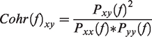
Coherence analysis, which is generally accepted as an indicator of functional corticocortical connections, e.g., increased coherence, is thought to reflect increased FC.^77–79 In this study, coherence analysis was employed as an essential indicator of laminar-specific interhemispheric FC and of which layer patterns between the symmetric cortices appeared in different ranges of low-frequency (<0.1 Hz). Layer-wise fMRI line profiles were used and converted to the Z-score normalized line profiles to minimize the dependency of the differences of baseline signal intensity between the left and right cortices. The coherence is defined as follows:

{Cohr (f)}_{x y} = \frac{{|P_{x y} (f)|}^{2}}{P_{x x} (f) {* P}_{y y} (f)}

where

x, y

indicates the Z-score normalized fMRI time series from each cortical region, and

P_{x x} (f)

P_{y y} (f)

is the individual PSD, and

P_{x y} (f)

is the cross PSD. The coherence was calculated by ‘mscohere’ function in MATLAB (Hamming window length: 2560, FFT length: 2000, overlap: 50%). To obviously compare the coherence results of two groups in evoked fMRI, the highest and least values of the coherence for each group was assigned to one and zero, respectively⁸⁰ (Figure 2(f) and (g)). The frequency resolution of the coherence was 1/200 s = 0.005 Hz which provides the capability to observe slow oscillatory frequencies. Fisher-Z transform was applied prior to averaging coherence and correlation coefficients with multiple trials.⁸¹

Figure 2.

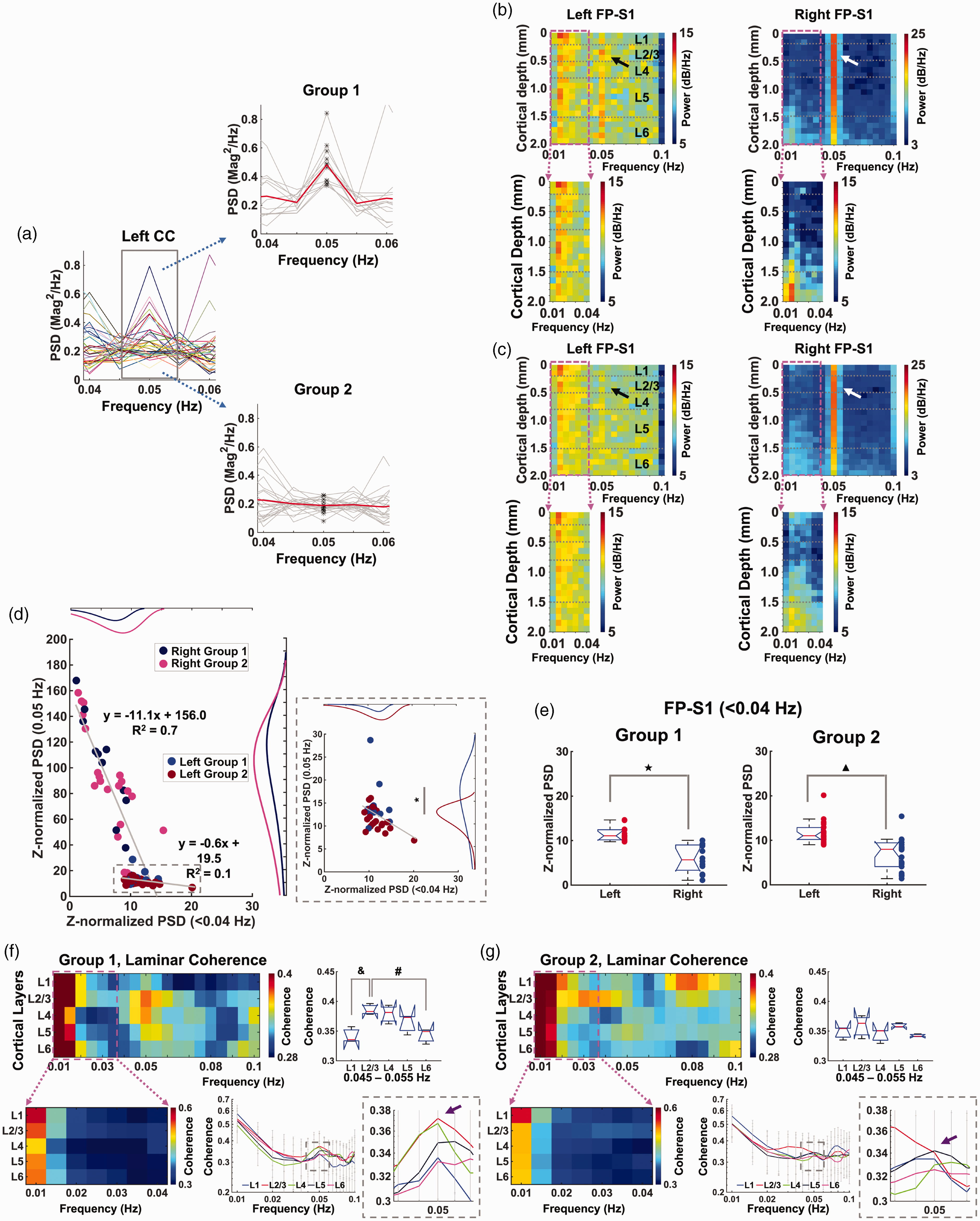
Corpus callosum activation-based grouping to characterize laminar-specific coherence patterns. (a) Left: PSD plots (0.04–0.06 Hz) of the filtered fMRI time series (average of 3 voxels, bandpass: 0.01–0.1 Hz) in the left corpus callosum to identify the stimulation frequency (0.05 Hz, n = 34 trials of 6 rats). Right: Corpus callosum activation-based grouping: Group 1 (upper) has the 0.05 Hz stimulation frequency, but Group 2 (lower) does not (Student t-test: p = 3.8 * 10⁻⁹, red line: mean, gray lines: individual trials, black points: values at 0.05 Hz). (b and c) Top: Voxel-wise Z-score normalized PSDs of the filtered time series (20 voxels, bandpass: 0.01–0.1 Hz) in the left and right FP-S1 from Group 1 (12 trials) and Group 2 (22 trials), respectively. Bottom: Enlarged voxel-wise PSDsContinued.(0.01–0.04 Hz) in the left and right FP-S1 of the corresponding groups (dashed box). (d) Scatter plots of Z-normalized PSDs in the left and right FP-S1: ultra-slow oscillation (<0.04 Hz) vs. stimulation-evoked BOLD responses (0.05 Hz) in Group 1 and 2. Individual dots represent trials. Dashed box: Enlarged scatter plot of the left FP-S1. Histogram fitting plots show distribution of the PSD values of Group 1 (left: blue, right: navy) and 2 (left: brown, right: magenta). Stimulation-evoked BOLD responses (0.05 Hz) show significant difference (Student t-test: *p = 0.025). (e) Comparison of Z-normalized PSDs of ultra-slow oscillation (<0.04 Hz) in the left (red) and right (blue) FP-S1 of Group 1 and 2 (Student t-test: ^★, ^▲ p < 10⁻⁴). f and g. Top-left: Group-averaged results representing laminar-specific coherence across the layers (L1, L2/3, L4, L5, L6) in Group 1 (f) and 2 (g). Top-right: Quantitative comparison of the laminar-specific coherences at 0.045-0.055 Hz. L2/3 is significantly different from L1 and L6 (one-way ANOVA: p = 0.02, post-hoc: ^{&, #}p < 0.05, Bonferroni correction) in Group 1 (f), meanwhile there is no significance in Group 2 (g). Bottom-left: Enlarged view of coherence in the ultra-slow oscillation (0.01–0.04 Hz) to clearly show the laminar-specific coherence patterns of Group 1 (f) and Group 2 (g). Bottom-right: Averaged layer-wise coherence plot of Group 1 (f) and Group 2 (g). Error bars represent mean ± SD across 6 animals. The purple arrows indicate the layer-wise coherence values at the stimulation-evoked frequency (0.05 Hz).

For clustering in rs-fMRI, the Gaussian Mixture Model clustering method was implemented in MATLAB and applied after preprocessing the coherence scatter points (Figure 3(g)). The expectation-maximization algorithm was used for fitting the mixture of Gaussian models to the data.^82,83

Figure 3.

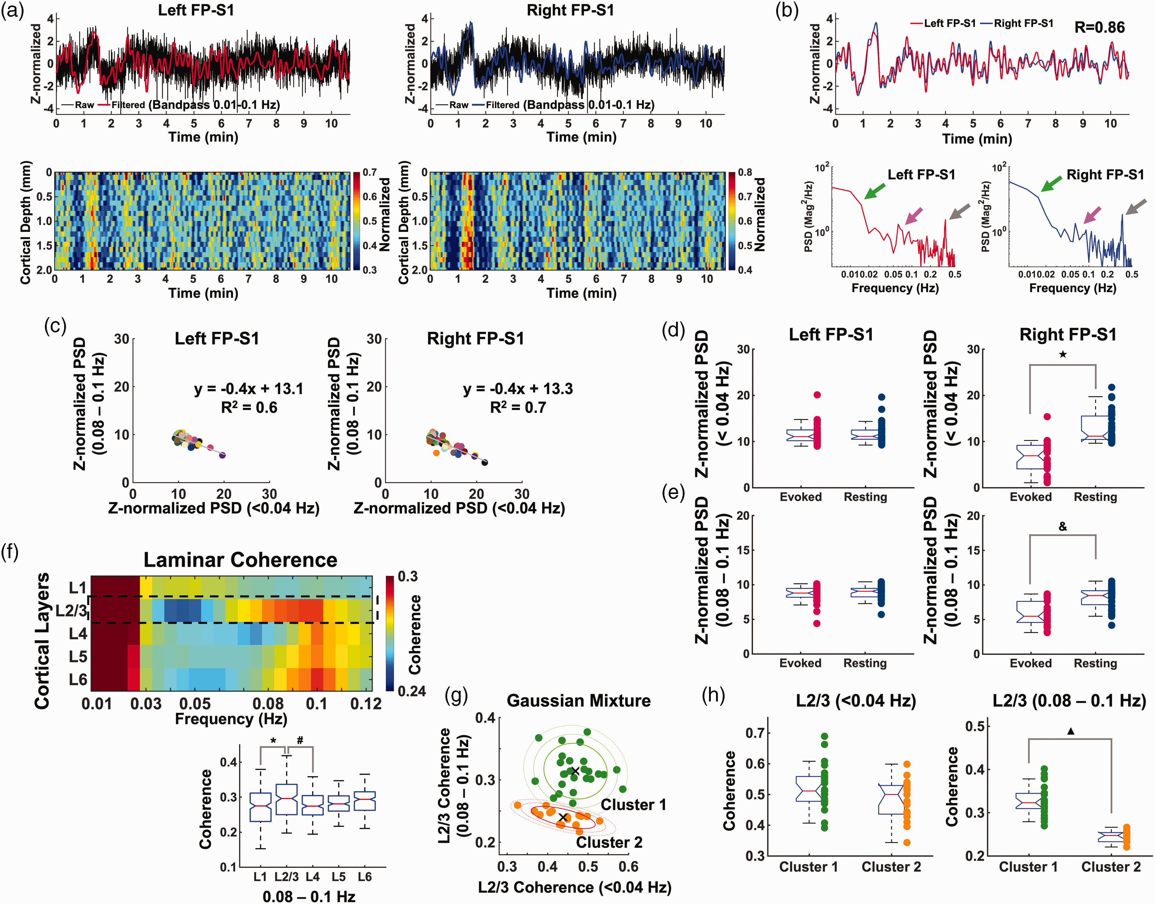
Characteristics of laminar-specific coherences in rs-fMRI using BiLS method. (a) Top: Z-score normalized fMRI time series of raw (black) and filtered (red and blue) data (average of 20 voxels, 0–2 mm, bandpass: 0.01–0.1 Hz) in the left and right FP-S1 during rest (10 min 40 sec, one representative trial). Bottom: Normalized spatiotemporal maps showing the laminar-specific responses across the cortical depth in the same FP-S1 (0–2 mm, bandpass: 0.01–0.1 Hz). (b) Top: Z-score normalized fMRI time series of the filtered data from the same trial in the left and right FP-S1 marked in red and blue, respectively (correlation: 0.86). Bottom: The PSD analyses of the Z-score normalized time series in both the left and right cortices show obvious peaks at the ultra-slow oscillatory frequency (green arrow, <0.04 Hz), 0.08–0.1 Hz (magenta arrow) and ∼0.3–0.4 Hz (gray arrow). (c) Scatter plots of Z-normalized PSDs in the left and right FP-S1: ultra-slow oscillation (<0.04 Hz) vs. 0.08–0.1 Hz in Group 1 and 2. Individual dots represent trials. (d) Comparison of Z-normalized PSDs of ultra-slow oscillation (<0.04 Hz) in the evoked (red) and rs- (navy) fMRI of Group 1 and 2 (t-test: ^★p < 10⁻¹⁰). (e) Comparison of Z-normalized PSDs of 0.08–0.1 Hz in the evoked (red) and rs- (navy) fMRI of Group 1 and 2 (t-test: ^&p < 10⁻⁷). (f–h) Average results of coherence from all data sets (n = 43 trials of 6 rats) (f) Top: Laminar-specific coherence across L1, L2/3, L4, L5, L6. Bottom: the average coherences (0.08–0.1 Hz) across the whole trials showing that L2/3 was significantly different from L1 and L4 (one-way ANOVA: p = 5.5 * 10⁻⁶, post-hoc: *p and ^#p < 0.05, Bonferroni correction). (g) Left: Scatter plot of the L2/3-specific coherence values with x-axis as the mean of coherence at <0.04 Hz and y-axis as the mean of coherence at 0.08–0.1 Hz to examine the dependence of the two different frequency bands. Right: By applying the Gaussian Mixture Model clustering with the L2/3 coherence values, all the 43 trials were divided into two groups. Cluster 1 (n = 26 trials) had relatively high averaged coherence values in both the frequency bands while Cluster 2 (n = 17 trials) had low averaged coherence values. ‘×’ signs indicate the centroid of the individual groups and (h) Cluster 1 and 2 show no significant difference at <0.04 Hz (left, independent t-test, p = 0.0805) while significant difference at 0.08–0.1 Hz (right, independent t-test, ^▲ p = 7.5853*10⁻¹²).

For statistical analysis, one-way ANOVA was performed to compare the layer-wise coherence values by using the post-hoc test in the evoked and rs-fMRI data. The coherence plot with error bars is displayed as the individual means ± SD. An independent samples t-test was applied to compare the means of two independent groups and to determine whether there was a statistically significant difference between the associated population means. Student t-test was performed to calculate a p-value. The p-values <0.05 were considered statistically significant. Fisher-Z transform was applied before testing one-way ANOVA and student t-test to meet the model assumption (i.e., normal distribution). No randomization design was needed in this work.

Results

Mapping the evoked BOLD fMRI signals with bilateral line-scanning fMRI

We developed a BiLS method to specify the high spatiotemporal resolution BOLD-fMRI signal at the forepaw somatosensory cortex (FP-S1). Figure 1(a) depicted the previous line-scanning scheme with two saturation slices to control the width of a FOV and to suppress signals outside the FOV. Figure 1(b) demonstrated FP-S1 BOLD responses across different cortical layers from the representative trial and averaged 2D fMRI maps. Figure 1(c) and (e) demonstrated the bilateral FP-S1 BOLD signals upon left forepaw electrical stimulation with the BiLS method, showing dynamic BOLD responses as a function of time in the FP-S1 of both hemispheres. In contrast to highly robust BOLD signals in right FP-S1 (4 s on/16 s off for each 20 s epoch), the ultra-slow oscillation of baseline fMRI signals was observed in the left FP-S1 ipsilateral to stimulation (Figure 1(c) and (d)). PSD analysis of bilateral FP-S1 showed a 0.05 Hz peak (Figure 1(f), magenta arrows) given the 20 s stimulation paradigm for each epoch. Meanwhile, PSD peaks of the ultra-slow fluctuation (<0.04 Hz) were detected in both FP-S1 (Figure 1(f), green arrows), which has been previously reported in anesthetized rats during rest.⁷⁵ This result demonstrated the feasibility of BiLS to acquire the interhemispheric laminar-specific fMRI signals with high spatiotemporal resolution. It should also be noted that the fast-sampling of the line-scanning scheme enables estimating the impact of cardiac and respiratory cycles on the rs-fMRI signal fluctuation. We had monitored respirations and blood pressures during fMRI experiments to calculate the spectrogram of the cardiorespiratory responses presenting 5–8 Hz cardiac and 1 Hz respiratory cycles of the anesthetized rats under ventilation (Figure S1 A and B).⁸⁴ The potential cardiac-related pulsation effect could be identified at the superficial L1, but was diminished in deeper layers (Figure S1 C).^85,86 Also, due to the usage of muscle relaxer during ventilation,⁶¹ the artifacts due to respiration-related B0 fluctuations^87,88 was negligible in line-scanning fMRI signals.

Mapping bilateral laminar BOLD responses based on CC activation

Using the BiLS method, we first focused on analyzing the interaction of laminar-specific BOLD fMRI signals through callosal projections with electrical stimulation of the left forepaw. We created a 2D line profile map to cover both gray matter (cortex, FP-S1) and white matter (corpus callosum, CC). As shown in Figure S2 A and B, the grayscale functional maps demonstrated different T2*-weighted signal intensity of cortical and CC regions given their different T2* values, presenting the dynamic fMRI responses in the color maps (details in Methods). From the representative trial, Z-score normalized fMRI signals (Figure S2 C–F) from FP-S1 and CC of two hemispheres were extracted to highlight the evoked BOLD signal at 0.05 Hz in the right FP-S1, while showing the relatively suppressed ultra-slow oscillation pattern (0.01–0.04 Hz) in the right (i.e., contralateral) FP-S1 (Figure S2 G). Besides the evoked BOLD in the right FP-S1 contralateral to the stimulation side, the left FP-S1 ipsilateral to the stimulation also showed 0.05 Hz evoked BOLD signal (Figure S2 G), but not all trials showed robust 0.05 Hz peaks through transcallosal projections. Figure S3 showed another representative trial with strong evoked BOLD signals in the right FP-S1 but not in the left side while showing the similar ultra-slow oscillatory patterns across two homologous FP-S1 regions (Figure S3 G).

To study the interhemispheric BOLD signal upon periodic stimulation at 0.05 Hz, we first investigated the CC activation-dependent laminar-specific interactions among different experimental trials. Based on the BOLD signals detected in the CC ipsilateral to stimulation, we sorted all the trials into two groups, i.e., with or without the 0.05 Hz peak in the PSD. As shown in Figure 2(a), Group 1 (12 trials) showed peaked power at 0.05 Hz with normalized values at 0.204 ± 0.122 (mean ± SD), which was significantly higher than other trials in Group 2 (22 trials, 0.190 ± 0.048) without a detectable peak. Figure 2(b) and (c) showed the color-coded power spectral maps with Z-score normalization across different cortical layers, demonstrating a salient peak at 0.05 Hz in the right FP-S1 of both groups⁸⁹ (Figure 2(b) and (c); white arrows, Figure S2 G and S3 G, Figure S8 A and B; gray arrows); however, the 0.05 Hz peak was only detected in the left FP-S1 of Group 1, but not in Group 2 (Figure 2(b) and (c), black arrows, Figure S2 G and S3 G, Figure S8 A and B; green arrows). In contrast, the ultra-slow oscillation (<0.04 Hz) in both FP-S1 regions was reliably detected in both groups (Figure 2(b) and (c)). Next, we analyzed the interaction of periodic stimulation-evoked BOLD responses (0.05 Hz) and ultra-slow oscillation (<0.04 Hz) by plotting their power levels cross different trials, showing negative correlation of both sides of FP-S1 (Figure 2(d)). Also, the power of the ultra-slow oscillation is significantly lower in the right FP-S1 than that in the left FP-S1 (Figure 2(e)). The laminar-specific reduction of ultra-slow oscillation power was detected from superficial layer to deep cortical L5 (Figure 2(b) and (c), S5 A and B).

Furthermore, we performed laminar-specific coherence analysis, showing that L2/3 and L4 had a strong peak at 0.05 Hz in Group 1, but not in Group 2 (Figure 2(f) and (g)). Laminar-specific coherence analysis between two FP-S1 regions revealed higher coherence coefficients at ultra-slow oscillation (<0.04 Hz) were across all cortical layers in both groups, but the coherence coefficient peaked at 0.05 Hz in Group 1 were primarily located at L2/3 which was higher than other layers (significance: p-value < 0.05, Figure 2(f)). As previously reported, 80% of callosal projection neurons (CPN) are located in L2/3,⁷⁴ explaining the strong coherence in the L2/3 of Group 1. Also, noteworthy was that the coherence coefficients of Group 2 showed higher values in L1 at 0.08–0.1 Hz than other layers, but not specific to 0.05 Hz (Figure 2(g)). In addition, Group 1 showed negative correlations between superficial layers of right FP-S1 and all the layers of left FP-S1 (Figure S4 A), possibly highlighting the transcallosal postsynaptic inhibitory effect in a delayed time scale negatively coupled to the BOLD signal detected in the draining veins of activated right FP-S1. It should be noted that the spectral analysis of Group 1 and 2 shows similar power levels of the ipsilateral ultra-slow oscillation (Figure 2(d)) and contralateral evoked BOLD responses (Figure 2(d), 0.05 Hz histogram plots). Spectral power plots between the different bandwidths (0.01–0.02 Hz, 0.02–0.04 Hz, and 0.08–0.1 Hz) of ipsilateral FP-S1 infraslow oscillation and evoked 0.05 Hz at the contralateral FP-S1 do not show linear correlation (Figure S7). Both results indicate that different coherence patterns between Group 1 and 2 across cortical layers do not depend on the infraslow oscillation or evoked BOLD responses. In summary, these results not only demonstrated the coexistence and interaction of the ultra-slow oscillation (<0.04 Hz) and evoked BOLD signal at 0.05 Hz, but also highlighted a CC activation-dependent L2/3-specific interhemispheric coherence pattern (Group 1) specific to the periodic stimulation.

Mapping laminar-specific bilateral functional connectivity at different frequencies during rest

Besides CC activation-dependent interhemispheric interaction, we investigated the laminar-specific bilateral rs-fMRI signals in anesthetized rats. Figure 3(a) showed representative Z-score normalized time courses from bilateral FP-S1, as well as 2D line profile rs-fMRI maps. The bilateral fMRI signal fluctuation peaked at <0.04 Hz and 0.08–0.1 Hz in PSD plots of both FP-S1 (Figure 3(b)). We plotted the power of ultra-slow oscillation (<0.04 Hz) versus the power of 0.08–0.1 Hz of the rs-fMRI signals in both FP-S1 across all trials (Figure 3(c)). Negative correlation of the two distinct fluctuation bandwidths showed a similar pattern to the previous experiment with periodic stimulation at 0.05 Hz block design. Also, the mean power of the infraslow frequency oscillation (<0.04 Hz and 0.08–0.1 Hz) of rs-fMRI at the contralateral FP-S1 is significantly higher than that of the experiment with periodic stimulation (Figure 3(d) and (e)), further indicating the regulation of the infraslow frequency oscillation by local cortical activation. We also performed the laminar-specific coherence analysis and revealed strong coherence of bilateral ultra-slow oscillation signals less than 0.04 Hz across all layers. Also, significantly higher coherence coefficients of 0.08–0.1 Hz were detected at L2/3 and the other layers (Figure 3(f)). Importantly, when plotting the trial-by-trial coherence coefficients at <0.04 Hz and 0.08–0.1 Hz, we observed two clusters of the recorded trials using Gaussian Mixture Model clustering method⁸² (Figure 3(g)). The two-spectral plots showed largely varied coherence of 0.08–0.1 Hz at L2/3 across different trials, presenting significantly higher coherence coefficient at Cluster 1 than that of Cluster 2, but little difference was observed for the ultra-slow oscillation between two clusters (Figure 3(h)). These results further demonstrated interhemispheric rs-fMRI connectivity can be specified at laminar-specific manner based on the underlying callosal projection, of which the variability of L2/3 coherence do not rely on the ultra-slow oscillation.

Discussion

We applied the BiLS method to investigate circuit-specific interhemispheric interaction of bilateral fMRI signals in anesthetized rats. Laminar-specific coherence analysis demonstrates two independent low-frequency oscillatory patterns. One is the ultra-slow oscillation less than 0.04 Hz across all cortical layers in both stimulation and resting conditions. The other is the L2/3-specific coherence pattern, which appeared at the 0.05 Hz according to the periodic stimulation, or at the 0.08–0.1 Hz bandwidth during rest. Although the ultra-slow oscillation is negatively correlated to the evoked BOLD signal based on periodic stimulation,^90–92 trial-specific analysis of the L2/3-specific coherence pattern in both conditions is not associated with the ultra-slow oscillation, indicating that the laminar-specific interhemispheric interaction is likely caused by different neuronal sources, e.g., callosal projection neurons.^73,74

Two challenging issues have limited the laminar-specific FC studies in rodent brains. First, fMRI is typically performed with a spatial resolution of several hundreds of microns,^93–96 and the conventional EPI-based fMRI is often performed with the temporal resolutions of 1–2 s.^37,97,98 The limited spatial or temporal resolution makes it difficult to elucidate circuit-specific interhemispheric FC. Even though very high spatial resolution can be achieved at the cost of a slow sampling rate,^46,52,99,100 the rs-fMRI signal is possibly confounded by the aliased cardiorespiratory artifacts.^61,85–88 Secondly, the high temporal signal to noise ratio (tSNR) is needed for correlation/coherence analysis of rs-fMRI signal for FC mapping.^101–103 In contrast to task-related fMRI experiments with massive averaging to increase the tSNR, it remains a challenge to achieve sufficient tSNR for rs-fMRI with high spatiotemporal resolution at a single trial. Also, trial-by-trial variability will be pivotal to be verified when statistical analysis is used to extract the general traits of the connectivity pattern based on the neuronal source.^91,104 To overcome these problems, the line-scanning scheme provides a critical mapping strategy to record laminar fMRI signals along the cortical depth in high spatiotemporal resolution and with sufficient tSNR.¹⁰⁵

Technical advances at the ultra-high magnetic field (e.g., 14T) in combination with focal MRI signal acquisition provide an excellent opportunity to study the laminar-specific interhemispheric FC. As shown in Figure S2, the gray matter (0–2 mm) and corpus callosum (2.0–2.3 mm) of FP-S1 were identified with the BiLS method. It is noteworthy that the temporal resolution of BiLS allows to eliminate the potential artifacts by temporal band-passed filters without concerning aliasing effect (Figure S1 C).^1,106 The artifact caused by cardiac pulsations are usually linked to large arteries located at the cortical surface.^85,86,107 As represented in Figure S1, the fast-sampling line-scanning scheme enables to detect laminar-specific pulsation-related artifacts (i.e., the 5–8 Hz cardiac cycles in rodents),⁶⁵ which are primarily located at L1. The lack of confounding artifacts to the laminar-specific rs-fMRI signal, especially at cortical layers deeper than L2/3, provides a unique platform to investigate the circuit-specific interhemispheric FC. Also, the laminar coherence map of Group 2 highlighted the superficial layer (L1) (Figure 2(g)), which may involve the non-neuronal BOLD signals from cardiovascular responses. Meanwhile, given GRE based MR sequences, large draining veins located in superficial layer result in higher signal fluctuation and spreading temporal responses which may also contribute to this observation.⁴⁸

Despite extensive studies to elucidate the transcallosal-mediated interhemispheric neuronal interactions,^{10,11,73,108,109} CC-dependent interhemispheric rs-fMRI FC were primarily verified based on loss-of-functional studies in acallosal patients^11–14 or animals with callosotomy.^15–17 The observation of maintaining interhemispheric FC in several rs-fMRI studies^11–13 raised the need to specify circuit-specific rs-fMRI signal fluctuations, in particular, when originating from varied neuronal sources. Using the BiLS method, we decomposed the bilateral low-frequency rs-fMRI signal fluctuation with laminar specificity, revealing two independent slow oscillatory patterns (i.e., ultra-slow oscillation <0.04 Hz and 0.08–0.1 Hz) possibly driven by different regulatory mechanisms (Figure 3). Callosal projection neurons are primarily located in L2/3 and project to both L2/3 and L5 of the opposite hemisphere,^74,110 which is well-matched with the detected laminar fMRI coherence peaks significantly located at L2/3, and partially at L5 (Figure 2(f)). Also, callosal circuit-specific optogenetic stimulation increased the power of the gamma frequency in L2/3 and L5 neurons,¹¹¹ and mediated unique BOLD response patterns through ortho- and anti-dromic projections.⁹⁷ Besides CC, there are a few brain structures connecting the two cerebral hemispheres such as anterior commissure, cingulum, interhemispheric thalamic connections. Major thalamocortical input target L4 of FP-S1 regions,^{50,52,53,112,113} leading to synchronized neuronal activity^72,114 (Figure 2(f), e.g., L4 has higher coherence values in Group 1 besides L2/3). A future study to combine the callosal circuit-specific optogenetic stimulation with BiLS will further elucidate the causal relationship, of which thalamocortical circuit optogenetic stimulation can be used as a control condition for laminar BOLD responses mapping with BiLS.

Robust ultra-slow oscillation (<0.04 Hz) across all the cortical layers with the BiLS method is consistent with the global BOLD signal fluctuation in anesthetized rats,⁷⁵ although the bandwidth (<0.015 Hz) signal fluctuation can be dampened at deeper anesthetized states. This ultra-slow oscillation was detected across different trials with or without peripheral stimulation, but its power was negatively correlated with evoked BOLD signal responses at 0.05 Hz, which are consistent with previous studies.^90–92 Moreover, the reduced ultra-slow oscillation at contralateral FP-S1 upon stimulation is consistent with previous calcium imaging study to measure the low-frequency global signal fluctuation with periodic stimulation.⁴² However, the ipsilateral ultra-slow oscillation was not suppressed by peripheral stimulation in our observation (Figures 2(e), 3(d) and (e)). Also, the spectral power plot between evoked 0.05 Hz responses in contralateral FP-S1 and layer-specific ultra-slow oscillation in the ipsilateral FP-S1 shows no linear correlation (Figure S7). It is possible that the large variability of ultra-slow rs-fMRI oscillation detected in the ipsilateral FP-S1 is mainly caused by brain state changes in anesthetized rats independent of the peripheral stimulation. This global signal fluctuation at ultra-slow frequency has been correlated with the brain-wide neuronal oscillatory sources in a brain state-dependent manner across different species.^75,115–117 Both subcortical neuronal projections through direct neuromodulation^{28,34,118,119} and autonomic regulation^38,120,121 could converge their regulatory effect to mediate the ultra-slow oscillatory patterns across cortical layers.^31–36 Interestingly, the L2/3-specific bilateral coherence patterns in both stimulation and resting states did not rely on the ultra-slow oscillation (Figures 2(e) and 3(h)). Our results further specified the distinct regulatory mechanisms underlying the ultra-slow oscillation across all cortical layers versus the L2/3-specific bilateral functional connectivity related to callosal projections.

It should be noted that the nature of the local neuronal circuitry that generates interhemispheric fluctuations and modulates the frequency bands of rs-fMRI signals remains an open issue.⁷ Nir and colleagues reported the low-frequency modulation in spontaneous firing rate and gamma LFP (40–100 Hz) as potential neural correlates of interhemispheric rs-fMRI signal fluctuation in the human sensory cortex.¹²² Similarly, Mateo and colleagues also reported gamma-rhythm oscillations at ∼0.1 Hz rhythm through vasomotion may serve as the underlying mechanism of the low-frequency hemodynamic signal fluctuation.^7,8 This has been further specified with the arteriole-specific single-vessel rs-fMRI study in anesthetized rats.⁷⁵ Moreover, hemodynamic signals correlate tightly with synchronized gamma oscillations in cats¹²³ and monkeys.¹¹⁷ Interestingly, Schoelvinck and colleagues reported that the LFP power of upper gamma-range frequency (40-80 Hz) and lower frequency range at 2–15 Hz recorded from a single cortical site were positively correlated with global rs-fMRI signals.¹¹⁷ This series of studies have provided strong evidence of the temporal neural correlation of rs-fMRI signal fluctuation. In our rs-fMRI study, the coherence pattern at 0.08–0.1 Hz is layer-specific, showing the broader and higher values at L2/3 (Figure 3(f)). It is possible that vasomotion at ∼0.1 Hz rhythm contributes to interhemispheric rs-fMRI signal fluctuation at 0.08–0.1 Hz across cortical layers.^{7,8,124–126} It should be noted that other non-neuronal oscillatory sources, e.g., Mayer waves that are tightly coupled with sympathetic nerve activity and arterial blood pressure, present slow oscillation across broad bandwidths. Previous studies have demonstrated typical ∼0.4 Hz Mayer waves in anesthetized rats.^80,127 In the power spectral plots, we have also observed Mayer waves at ∼0.3–0.4 Hz in both evoked and rs-fMRI (Figure S8). It is noteworthy that the Mayer waves at ∼0.3–0.4 Hz appear bilaterally from superficial layer to deeper layer in both evoked and rs-fMRI (Figure 3(b) and S9–11). The above-mentioned studies do not assign the frequency-specific fluctuation to underlying neural projection circuits, which is critical to verify the distinct neural basis of FC. Our study, for the first time, shows the frequency-specific oscillatory patterns across different cortical layers, presenting an important step to elucidate the neuronal circuit basis of the FC with rs-fMRI.

Several limitations about the BiLS method should be considered when interpreting the results of this study and for future optimization using high field rs-fMRI studies. Firstly, because of usage of saturation slices to delineate the FOV, adiabatic RF pulses are needed to produce sufficient and uniform signal saturation outside of the FOV. Alternative mapping strategy using 90–180° spin-echo-based line-scanning scheme will be further explored in multi-slice line-scanning acquisition.¹⁰⁵ Secondly, due to the poor homogeneity of high magnetic field and different draining vein distribution on cortical surface across animals, tSNR can vary across line profiles from two hemispheres. Also, the ultra-slow oscillation (<0.015 Hz) may not be well recorded with the 10 min line-scanning trial due to insufficient sampling acquisition and tSNR. To achieve sufficient tSNR, we can apply inductive coils¹²⁸ or wireless amplified NM detectors^129,130 by region-specific implantation. Thirdly, although we only focused on the anesthetized rodent brains, the line-scanning method has been applied for human brain mapping.^70,131 Despite cortical folds and fissures, it is possible to position the FOV to cover focal cortical regions and achieve laminar-specific fMRI signals with the multi-slice line-scanning scheme. Meanwhile, the multi-slice line-scanning scheme can be combined with the laminar electrophysiological recording or fiber photometry-based fluorescent recordings from genetically encoded biosensors, e.g., Ca²⁺, Glutamate, and dopamine,^75,132–134 to further elucidate the neuronal basis of the circuit-specific rs-fMRI FC. Lastly, we performed the BiLS studies only under a single anesthetic regimen (i.e., alpha-chloralose). The timing of each trial acquired during the anesthetic protocol has been listed in Table S1. Although the total anesthetic time experienced by animals did not contribute to the evoked BOLD signal in the left FP-S1, the callosal-mediated positive BOLD signal at L2/3 occurred at the relatively early stage of experiments (Figure S6). It is possible that different coherence patterns of trials in Group 1 and 2 may be influenced by the overall energy consumption of the brain along the long-hour experiments for anesthetized animals. In future work, we will apply the BiLS method to map rs- fMRI signals of awake mice, aiming to distinguish the bandwidth-specific FC without anesthetic effect.³⁹

Supplemental Material

sj-pdf-1-jcb-10.1177_0271678X231158434 - Supplemental material for Identifying the distinct spectral dynamics of laminar-specific interhemispheric connectivity with bilateral line-scanning fMRI

Supplemental material, sj-pdf-1-jcb-10.1177_0271678X231158434 for Identifying the distinct spectral dynamics of laminar-specific interhemispheric connectivity with bilateral line-scanning fMRI by Sangcheon Choi, Yi Chen, Hang Zeng, Bharat Biswal and Xin Yu in Journal of Cerebral Blood Flow & Metabolism

Footnotes

Funding

The author(s) disclosed receipt of the following financial support for the research, authorship, and/or publication of this article: This research was supported by NIH Brain Initiative funding (RF1NS113278-01, R01 MH111438-01), RF1NS124778, R01NS120594, R21NS121642, NSF grant 2123971, and the S10 instrument grant (S10 MH124733) to Martinos Center, German Research Foundation (DFG) Yu215/2-1, 3-1, BMBF 01GQ1702, and the internal funding from Max Planck Society. This project has received funding from the European Union Framework Programme for Research and Innovation Horizon 2020 (2014–2020) under the Marie Skłodowska-Curie Grant Agreement No.896245. We thank Dr. R. Pohmann, Dr. J. Engelmann, Dr. N. Avdievitch, and Ms. H. Schulz for technical support, Dr. P. Douay, Ms. R. König, and Ms. M. Pitscheider for animal support, the AFNI team for the software support.

Declaration of conflicting interests

The author(s) declared no potential conflicts of interest with respect to the research, authorship, and/or publication of this article.

Authors’ contributions

X.Y. designed and supervised the research, H.Z. and X.Y. performed animal experiments, S.C., Y.C., H.Z., and X.Y. acquired data, S.C. analyzed data, H.Z. and X.Y. provided technical support, X.Y., S.C., Y.C., and B.B. wrote the manuscript.

Code availability

The related image processing codes are available from the corresponding author upon reasonable request.

Data availability

All data generated during this study are available from the corresponding author upon reasonable request.

ORCID iD

Xin Yu

Supplemental material

Supplemental material for this article is available online.

References

Biswal

Yetkin

Haughton

, et al. Functional connectivity in the motor cortex of resting human brain using Echo-Planar mri. Magn Reson Med 1995; 34: 537–541.

Biswal

Mennes

Zuo

, et al. Toward discovery science of human brain function. Proc Natl Acad Sci U S A 2010; 107: 4734–4739.

Biswal

BB.

Resting state fMRI: a personal history. Neuroimage 2012; 62: 938–944.

Buckner

Krienen

Yeo

BT.

Opportunities and limitations of intrinsic functional connectivity MRI. Nat Neurosci 2013; 16: 832–837.

Fox

Raichle

ME.

Spontaneous fluctuations in brain activity observed with functional magnetic resonance imaging. Nat Rev Neurosci 2007; 8: 700–711.

Chuang

Nasrallah

FA.

Functional networks and network perturbations in rodents. Neuroimage 2017; 163: 419–436.

Drew

Mateo

Turner

, et al. Ultra-slow oscillations in fMRI and resting-state connectivity: neuronal and vascular contributions and technical confounds. Neuron 2020; 107: 782–804.

Mateo

Knutsen

Tsai

, et al. Entrainment of arteriole vasomotor fluctuations by neural activity is a basis of Blood-Oxygenation-Level-Dependent “Resting-State'' connectivity. Neuron 2017; 96: 936–948.e3.

Sforazzini

Schwarz

Galbusera

, et al. Distributed BOLD and CBV-weighted resting-state networks in the mouse brain. Neuroimage 2014; 87: 403–415.

10.

Baek

Shim

Jeong

, et al. Layer-specific interhemispheric functional connectivity in the somatosensory cortex of rats: resting state electrophysiology and fMRI studies. Brain Struct Funct 2016; 221: 2801–2815.

11.

Roland

Snyder

Hacker

, et al. On the role of the corpus callosum in interhemispheric functional connectivity in humans. Proc Natl Acad Sci U S A 2017; 114: 13278–13283.

12.

Owen

Yang

, et al. Resting-state networks and the functional connectome of the human brain in agenesis of the corpus callosum. Brain Connect 2013; 3: 547–562.

13.

Johnston

Vaishnavi

Smyth

, et al. Loss of resting interhemispheric functional connectivity after complete section of the corpus callosum. J Neurosci 2008; 28: 6453–6458.

14.

Quigley

Cordes

Turski

, et al. Role of the corpus callosum in functional connectivity. AJNR Am J Neuroradiol 2003; 24: 208–212.

15.

Magnuson

Thompson

Pan

, et al. Effects of severing the corpus callosum on electrical and BOLD functional connectivity and spontaneous dynamic activity in the rat brain. Brain Connect 2014; 4: 15–29.

16.

Zhou

Liang

Chan

, et al. Brain resting-state functional MRI connectivity: morphological foundation and plasticity. Neuroimage 2014; 84: 1–10.

17.

Sforazzini

Bertero

Dodero

, et al. Altered functional connectivity networks in acallosal and socially impaired BTBR mice. Brain Struct Funct 2016; 221: 941–954.

18.

Tyszka

Kennedy

Adolphs

, et al. Intact bilateral resting-state networks in the absence of the corpus callosum. J Neurosci 2011; 31: 15154–15162.

19.

Uddin

Mooshagian

Zaidel

, et al. Residual functional connectivity in the split-brain revealed with resting-state functional MRI. Neuroreport 2008; 19: 703–709.

20.

Khanna

Poliakov

Ishak

, et al. Preserved interhemispheric functional connectivity in a case of corpus callosum agenesis. Neuroradiology 2012; 54: 177–179.

21.

Tovar-Moll

Monteiro

Andrade

, et al. Structural and functional brain rewiring clarifies preserved interhemispheric transfer in humans born without the corpus callosum. Proc Natl Acad Sci U S A 2014; 111: 7843–7848.

22.

Corsi-Cabrera

Ondarza

Martinez-Gutierrez

, et al. Role of corpus callosum in interhemispheric coherent activity during sleep. Clin Neurophysiol 2006; 117: 1826–1835.

23.

O'Reilly

Croxson

Jbabdi

, et al. Causal effect of disconnection lesions on interhemispheric functional connectivity in rhesus monkeys. Proc Natl Acad Sci U S A 2013; 110: 13982–13987.

24.

Poulet

Fernandez

Crochet

, et al. Thalamic control of cortical states. Nat Neurosci 2012; 15: 370–372.

25.

Lee

Durand

Gradinaru

, et al. Global and local fMRI signals driven by neurons defined optogenetically by type and wiring. Nature 2010; 465: 788–792.

26.

Xiao

Vanni

Mitelut

, et al. Mapping cortical mesoscopic networks of single spiking cortical or sub-cortical neurons. Elife 2017; 6: e19976.

27.

Başar

Güntekin

A review of brain oscillations in cognitive disorders and the role of neurotransmitters. Brain Res 2008; 1235: 172–193.

28.

Turchi

Chang

, et al. The basal forebrain regulates global resting-state fMRI fluctuations. Neuron 2018; 97: 940–952 e944.

29.

Chang

Yang

, et al. Cortical modulation of motor control biofeedback among the elderly with high fall risk during a posture perturbation task with augmented reality. Front Aging Neurosci 2016; 8: 80.

30.

Rho

Kim

Lee

SH.

Function of selective neuromodulatory projections in the mammalian cerebral cortex: comparison between cholinergic and noradrenergic systems. Front Neural Circuits 2018; 12: 47.

31.

Schwarz

Luo

Organization of the locus coeruleus-norepinephrine system. Curr Biol 2015; 25: R1051–R1056.

32.

Honjoh

Sasai

Schiereck

, et al. Regulation of cortical activity and arousal by the matrix cells of the ventromedial thalamic nucleus. Nat Commun 2018; 9: 2100.

33.

Azimi

Klaassen

Thomas

, et al. Role of the thalamus in basal forebrain regulation of neural activity in the primary auditory cortex. Cereb Cortex 2020; 30: 4481–4495.

34.

Liu

de Zwart

Scholvinck

, et al. Subcortical evidence for a contribution of arousal to fMRI studies of brain activity. Nat Commun 2018; 9: 395.

35.

Kim

Thankachan

McKenna

, et al. Cortically projecting basal forebrain parvalbumin neurons regulate cortical gamma band oscillations. Proc Natl Acad Sci U S A 2015; 112: 3535–3540.

36.

Totah

Neves

Panzeri

, et al. The locus coeruleus is a complex and differentiated neuromodulatory system. Neuron 2018; 99: 1055–1068.e6.

37.

Wang

Sejnowski

, et al. Brain-state dependent astrocytic Ca(2+) signals are coupled to both positive and negative BOLD-fMRI signals. Proc Natl Acad Sci Usa 2018; 115: E1647–E1656.

38.

Pais-Roldan

Takahashi

Sobczak

, et al. Indexing brain state-dependent pupil dynamics with simultaneous fMRI and optical fiber calcium recording. Proc Natl Acad Sci Usa 2020; 117: 6875–6882.

39.

Mohajerani

Chan

Mohsenvand

, et al. Spontaneous cortical activity alternates between motifs defined by regional axonal projections. Nat Neurosci 2013; 16: 1426–1435.

40.

Zhang

Raichle

ME.

Disease and the brain's dark energy. Nat Rev Neurol 2010; 6: 15–28.

41.

Destexhe

Contreras

Neuronal computations with stochastic network states. Science 2006; 314: 85–90.

42.

Rosenthal

Raut

Bowen

, et al. Peripheral sensory stimulation elicits global slow waves by recruiting somatosensory cortex bilaterally. Proc Natl Acad Sci Usa 2021; 118: e2021252118.

43.

Huber

Handwerker

Jangraw

, et al. High-resolution CBV-fMRI allows mapping of laminar activity and connectivity of cortical input and output in human M1. Neuron 2017; 96: 1253–1263.e7.

44.

Sharoh

van Mourik

Bains

, et al. Laminar specific fMRI reveals directed interactions in distributed networks during language processing. Proc Natl Acad Sci U S A 2019; 116: 21185–21190.

45.

Finn

Huber

Jangraw

, et al. Layer-dependent activity in human prefrontal cortex during working memory. Nat Neurosci 2019; 22: 1687–1695.

46.

Kashyap

Ivanov

Havlicek

, et al. Resolving laminar activation in human V1 using ultra-high spatial resolution fMRI at 7T. Sci Rep-Uk 2018; 8: 17063.

47.

Huber

Yang

, et al. Layer-specific activation of sensory input and predictive feedback in the human primary somatosensory cortex. Sci Adv 2019; 5: eaav9053.

48.

Chen

Wang

Gore

, et al. Layer-specific BOLD activation in awake monkey V1 revealed by ultra-high spatial resolution functional magnetic resonance imaging. Neuroimage 2013; 64: 147–155.

49.

Goense

JBM

Logothetis

NK.

Laminar specificity in monkey V1 using high-resolution SE-fMRI. Magn Reson Imaging 2006; 24: 381–392.

50.

Qian

Chen

, et al. Deciphering laminar-specific neural inputs with line-scanning fMRI. Nat Methods 2014; 11: 55–58.

51.

Albers

Schmid

Wachsmuth

, et al. Line scanning fMRI reveals earlier onset of optogenetically evoked BOLD response in rat somatosensory cortex as compared to sensory stimulation. Neuroimage 2018; 164: 144–154.

52.

Silva

Koretsky

AP.

Laminar specificity of functional MRI onset times during somatosensory stimulation in rat. Proc Natl Acad Sci U S A 2002; 99: 15182–15187.

53.

Jung

Jiang

, et al. Early fMRI responses to somatosensory and optogenetic stimulation reflect neural information flow. Proc Natl Acad Sci USA 2021; 118: e2023265118.

54.

Glover

Ress

Image-based method for retrospective correction of physiological motion effects in fMRI: RETROICOR. Magn Reson Med 2000; 44: 162–167.

55.

Birn

Diamond

Smith

, et al. Separating respiratory-variation-related fluctuations from neuronal-activity-related fluctuations in fMRI. Neuroimage 2006; 31: 1536–1548.

56.

Chang

Cunningham

Glover

GH.

Influence of heart rate on the BOLD signal: the cardiac response function. Neuroimage 2009; 44: 857–869.

57.

Golestani

Chang

Kwinta

, et al. Mapping the end-tidal CO₂ response function in the resting-state BOLD fMRI signal: spatial specificity, test-retest reliability and effect of fMRI sampling rate. Neuroimage 2015; 104: 266–277.

58.

Blazejewska

Fischl

Wald

, et al. Intracortical smoothing of small-voxel fMRI data can provide increased detection power without spatial resolution losses compared to conventional large-voxel fMRI data. Neuroimage 2019; 189: 601–614.

59.

Koopmans

Barth

Orzada

, et al. Multi-echo fMRI of the cortical laminae in humans at 7 T. Neuroimage 2011; 56: 1276–1285.

60.

Guidi

Huber

Lampe

, et al. Cortical laminar resting-state signal fluctuations scale with the hypercapnic blood oxygenation level-dependent response. Hum Brain Mapp 2020; 41: 2014–2027.

61.

Pais-Roldan

Biswal

Scheffler

, et al. Identifying respiration-related aliasing artifacts in the rodent resting-state fMRI. Front Neurosci 2018; 12: 788.

62.

Zhao

Zhou

, et al. BOLD study of stimulation-induced neural activity and resting-state connectivity in medetomidine-sedated rat. Neuroimage 2008; 39: 248–260.

63.

Williams

Magnuson

Majeed

, et al. Comparison of alpha-chloralose, medetomidine and isoflurane anesthesia for functional connectivity mapping in the rat. Magn Reson Imaging 2010; 28: 995–1003.

64.

Bukhari

Schroeter

Cole

, et al. Resting state fMRI in mice reveals anesthesia specific signatures of brain functional networks and their interactions. Front Neural Circuits 2017; 11: 5.

65.

Kalthoff

Seehafer

, et al. Functional connectivity in the rat at 11.7T: impact of physiological noise in resting state fMRI. Neuroimage 2011; 54: 2828–2839.

66.

Fischl

Dale

AM.

Measuring the thickness of the human cerebral cortex from magnetic resonance images. Proc Natl Acad Sci U S A 2000; 97: 11050–11055.

67.

Raimondo

Knapen

Oliveira

, et al. Preliminary results of functional line-scanning in humans: submillimeter, subsecond resolution evoked responses. 36th Annu Scient Meeting Eur Soc Magn Reson Med Biol 2019; S22.06: S334.

68.

Siero

Oliveira

Choi

, et al. Implementing human line-scanning fMRI: initial results of ultra-high temporal and spatial resolution fMRI. Proc Intl Soc Mag Reson Med 2019; 27: 3933.

69.

Balasubramanian

Mulkern

Neil

, et al. Probing in vivo cortical myeloarchitecture in humans via line-scan diffusion acquisitions at 7 T with 250-500 micron radial resolution. Magn Reson Med 2021; 85: 390–403.

70.

Morgan

Nothnagel

Petro

, et al. High-resolution line-scanning reveals distinct visual response properties across human cortical layers. bioRxiv 2020; 2020.2006.2030: 179762.

71.

Whitesell

Liska

Coletta

, et al. Regional, layer, and cell-type-specific connectivity of the mouse default mode network. Neuron 2021; 109: 545–559 e548.

72.

Choi

Zeng

Chen

, et al. Laminar-specific functional connectivity mapping with multi-slice line-scanning fMRI. Cereb Cortex 2022; 32: 4492–4501.

73.

Bloom

Hynd

GW.

The role of the corpus callosum in interhemispheric transfer of information: excitation or inhibition?

Neuropsychol Rev 2005; 15: 59–71.

74.

Fame

MacDonald

Macklis

JD.

Development, specification, and diversity of callosal projection neurons. Trends Neurosci 2011; 34: 41–50.

75.

Wang

Chen

, et al. Ultra-slow single-vessel BOLD and CBV-based fMRI spatiotemporal dynamics and their correlation with neuronal intracellular calcium signals. Neuron 2018; 97: 925–939 e925.

76.

Cox

RW.

AFNI: software for analysis and visualization of functional magnetic resonance neuroimages. Comput Biomed Res 1996; 29: 162–173.

77.

Leocani

Comi

EEG coherence in pathological conditions. J Clin Neurophysiol 1999; 16: 548–555.

78.

Drew

Duyn

Golanov

, et al. Finding coherence in spontaneous oscillations. Nat Neurosci 2008; 11: 991–993.

79.

Wang

Saalmann

Pinsk

, et al. Electrophysiological low-frequency coherence and cross-frequency coupling contribute to BOLD connectivity. Neuron 2012; 76: 1010–1020.

80.

Brown

Patwardhan

, et al. Sympathetic activity and blood pressure are tightly coupled at 0.4 Hz in conscious rats. Am J Physiol 1994; 267: R1378–1384.

81.

Silver

Dunlap

WP.

Averaging correlation-coefficients – should fisher Z-transformation be used. J Appl Psychol 1987; 72: 146–148.

82.

McLachlan

Basford

KE.

Mixture models: inference and applications to clustering. Appl Stat 1988; 38: 384–385.

83.

Sobczak

Pais-Roldan

Takahashi

, et al. Decoding the brain state-dependent relationship between pupil dynamics and resting state fMRI signal fluctuation. Elife 2021; 10: e68980.

84.

Choi

Takahashi

Jiang

, et al. Real-time fMRI brain mapping in animals. JoVE 2020; 163: e61463.

85.

Murphy

Birn

Bandettini

PA.

Resting-state fMRI confounds and cleanup. Neuroimage 2013; 80: 349–359.

86.

Caballero-Gaudes

Reynolds

RC.

Methods for cleaning the BOLD fMRI signal. Neuroimage 2017; 154: 128–149.

87.

Raj

Anderson

Gore

JC.

Respiratory effects in human functional magnetic resonance imaging due to bulk susceptibility changes. Phys Med Biol 2001; 46: 3331–3340.

88.

Van de Moortele

Pfeuffer

Glover

, et al. Respiration-induced B0 fluctuations and their spatial distribution in the human brain at 7 tesla. Magn Reson Med 2002; 47: 888–895.

89.

Nasrallah

Tay

Chuang

KH.

Detection of functional connectivity in the resting mouse brain. Neuroimage 2014; 86: 417–424.

90.

Chen

Park

Pan

, et al. Interactions between stimuli-evoked cortical activity and spontaneous low frequency oscillations measured with neuronal calcium. Neuroimage 2020; 210: 116554.

91.

Shimaoka

Steinmetz

Harris

, et al. The impact of bilateral ongoing activity on evoked responses in mouse cortex. Elife 2019; 8: e43533.

92.

Petersen

Hahn

Mehta

, et al. Interaction of sensory responses with spontaneous depolarization in layer 2/3 barrel cortex. Proc Natl Acad Sci U S A 2003; 100: 13638–13643.

93.

Ogawa

Tank

Menon

, et al. Intrinsic signal changes accompanying sensory stimulation – functional brain mapping with magnetic-resonance-imaging. Proc Natl Acad Sci U S A 1992; 89: 5951–5955.

94.

Logothetis

Pauls

Augath

, et al. Neurophysiological investigation of the basis of the fMRI signal. Nature 2001; 412: 150–157.

95.

Logothetis

NK.

What we can do and what we cannot do with fMRI. Nature 2008; 453: 869–878.

96.

Gil

Fernandes

Shemesh

Neuroplasticity-driven timing modulations revealed by ultrafast functional magnetic resonance imaging. Neuroimage 2021; 225: 117446.

97.

Chen

Sobczak

Pais-Roldan

, et al. Mapping the brain-wide network effects by optogenetic activation of the corpus callosum. Cereb Cortex 2020; 30: 5885–5898.

98.

Jung

Shim

Kim

SG.

Mouse BOLD fMRI at ultrahigh field detects somatosensory networks including thalamic nuclei. Neuroimage 2019; 195: 203–214.

99.

Hirano

Stefanovic

Silva

AC.

Spatiotemporal evolution of the functional magnetic resonance imaging response to ultrashort stimuli. J Neurosci 2011; 31: 1440–1447.

100.

Poplawsky

Fukuda

Murphy

, et al. Layer-specific fMRI responses to excitatory and inhibitory neuronal activities in the olfactory bulb. J Neurosci 2015; 35: 15263–15275.

101.

Murphy

Bodurka

Bandettini

PA.

How long to scan? The relationship between fMRI temporal signal to noise ratio and necessary scan duration. Neuroimage 2007; 34: 565–574.

102.

Van Dijk

KRA

Hedden

Venkataraman

, et al. Intrinsic functional connectivity as a tool for human connectomics: theory, properties, and optimization. J Neurophysiol 2010; 103: 297–321.

103.

Fox

Snyder

Zacks

, et al. Coherent spontaneous activity accounts for trial-to-trial variability in human evoked brain responses. Nat Neurosci 2006; 9: 23–25.

104.

Paasonen

Salo

Huttunen

, et al. Resting-state functional MRI as a tool for evaluating brain hemodynamic responsiveness to external stimuli in rats. Magn Reson Med 2017; 78: 1136–1146.

105.

Choi

Zeng

Pohmann

, et al. Novel alpha-180 SE based LINE-scanning method (SELINE) for laminar-specific fMRI. Proc Intl Soc Mag Reson Med 2018; 27: 1166.

106.

Lowe

Mock

and Sorenson

JA.

Functional connectivity in single and multislice echoplanar imaging using resting-state fluctuations. NeuroImage 1998; 7: 119–132.

107.

Polimeni

Bianciardi

Keil

, et al. Cortical depth dependence of physiological fluctuations and whole-brain resting-state functional connectivity at 7T. Proc Intl Soc Mag Reson Med 2015; 23: 592.

108.

Caminiti

Ghaziri

Galuske

, et al. Evolution amplified processing with temporally dispersed slow neuronal connectivity in primates. Proc Natl Acad Sci U S A 2009; 106: 19551–19556.

109.

Hofer

Frahm

Topography of the human corpus callosum revisited – comprehensive fiber tractography using diffusion tensor magnetic resonance imaging. Neuroimage 2006; 32: 989–994.

110.

Hagihara

Ishikawa

Yoshimura

, et al. Long-range interhemispheric projection neurons show biased response properties and Fine-Scale local subnetworks in mouse visual cortex. Cereb Cortex 2021; 31: 1307–1315.

111.

Iordanova

Vazquez

Kozai

, et al. Optogenetic investigation of the variable neurovascular coupling along the interhemispheric circuits. J Cereb Blood Flow Metab 2018; 38: 627–640.

112.

Glen

Wang

, et al. Direct imaging of macrovascular and microvascular contributions to BOLD fMRI in layers IV-V of the rat whisker-barrel cortex. Neuroimage 2012; 59: 1451–1460.

113.

Jabaudon

Fate and freedom in developing neocortical circuits. Nat Commun 2017; 8: 16042.

114.

Bruno

Sakmann

Cortex is driven by weak but synchronously active thalamocortical synapses. Science 2006; 312: 1622–1627.

115.

Raichle

MacLeod

Snyder

, et al. A default mode of brain function. Proc Natl Acad Sci U S A 2001; 98: 676–682.

116.

Shaik

Kozberg

, et al. Resting-state hemodynamics are spatiotemporally coupled to synchronized and symmetric neural activity in excitatory neurons. Proc Natl Acad Sci U S A 2016; 113: E8463–E8471.

117.

Scholvinck

Maier

, et al. Neural basis of global resting-state fMRI activity. Proc Natl Acad Sci U S A 2010; 107: 10238–10243.

118.

Sun

, et al. Generation of a whole-brain atlas for the cholinergic system and mesoscopic projectome analysis of basal forebrain cholinergic neurons. Proc Natl Acad Sci U S A 2018; 115: 415–420.

119.

Williams

Nathans

Complete morphologies of basal forebrain cholinergic neurons in the mouse. Elife 2014; 3: e02444.

120.

Ozbay

Chang

Picchioni

, et al. Sympathetic activity contributes to the fMRI signal. Commun Biol 2019; 2: 421.

121.

Lewis

Lantigua

Atlas

, et al. A cross-sectional assessment to detect type 2 diabetes with endothelial and autonomic nervous system markers using a novel system. J Diabetes Metab Disord 2014; 13: 118.

122.

Nir

Mukamel

Dinstein

, et al. Interhemispheric correlations of slow spontaneous neuronal fluctuations revealed in human sensory cortex. Nat Neurosci 2008; 11: 1100–1108.

123.

Niessing

Ebisch

Schmidt

, et al. Hemodynamic signals correlate tightly with synchronized gamma oscillations. Science 2005; 309: 948–951.

124.

Bumstead

Bauer

Wright

, et al. Cerebral functional connectivity and Mayer waves in mice: phenomena and separability. J Cereb Blood Flow Metab 2017; 37: 471–484.

125.

Mayhew

Askew

Zheng

, et al. Cerebral vasomotion: a 0.1-Hz oscillation in reflected light imaging of neural activity. Neuroimage 1996; 4: 183–193.

126.

Nilsson

Aalkjaer

Vasomotion: mechanisms and physiological importance. Mol Interv 2003; 3: 79–89, 51.

127.

Julien

The enigma of Mayer waves: facts and models. Cardiovasc Res 2006; 70: 12–21.

128.

Inigo-Marco

Isturiz

Fernandez

, et al. Imaging of stroke in rodents using a clinical scanner and inductively coupled specially designed receiver coils. Annals of Biomedical Engineering 2020; 49: 746–756.

129.

Qian

CQ.

Wireless reconfigurable RF detector array for focal and multiregional signal enhancement. Ieee Access 2020; 8: 136594–136604.

130.

Qian

Chen

, et al. Wireless amplified nuclear MR detector (WAND) for high-spatial-resolution MR imaging of internal organs: preclinical demonstration in a rodent model. Radiology 2013; 268: 228–236.

131.

Raimondo

Knapen

Oliveira

IAF

, et al. A line through the brain: implementation of human line-scanning at 7T for ultra-high spatiotemporal resolution fMRI. J Cereb Blood Flow Metab 2021; 41: 2831–2843.

132.

Jiang

Chen

Pais Roldán

, et al. Deciphering the contribution of extracellular glutamate and intracellular calcium signaling to the BOLD fMRI signal. ISMRM SMRT Virtual Conf Exhib 2020; 28: 1340.

133.

Sun

Zeng

Jing

, et al. A genetically encoded fluorescent sensor enables rapid and specific detection of dopamine in flies, fish, and mice. Cell 2018; 174: 481–496 e419.

134.

Patriarchi

Cho

Merten

, et al. Ultrafast neuronal imaging of dopamine dynamics with designed genetically encoded sensors. Science 2018; 360: eaat4422.

Supplementary Material

Please find the following supplemental material available below.

For Open Access articles published under a Creative Commons License, all supplemental material carries the same license as the article it is associated with.

For non-Open Access articles published, all supplemental material carries a non-exclusive license, and permission requests for re-use of supplemental material or any part of supplemental material shall be sent directly to the copyright owner as specified in the copyright notice associated with the article.

0.00 MB

2.87 MB