Sage Journals: Discover world-class research

Abstract

Advances in deep learning can be applied to acute stroke imaging to build powerful and explainable prediction models that could supersede traditionally used biomarkers. We aimed to evaluate the performance and interpretability of a deep learning model based on convolutional neural networks (CNN) in predicting long-term functional outcome with diffusion-weighted imaging (DWI) acquired at day 1 post-stroke. Ischemic stroke patients (n = 322) were included from the ASTER and INSULINFARCT trials as well as the Pitié-Salpêtrière registry. We trained a CNN to predict long-term functional outcome assessed at 3 months with the modified Rankin Scale (dichotomized as good [mRS ≤ 2] vs. poor [mRS ≥ 3]) and compared its performance to two logistic regression models using lesion volume and ASPECTS. The CNN contained an attention mechanism, which allowed to visualize the areas of the brain that drove prediction. The deep learning model yielded a significantly higher area under the curve (0.83 95%CI [0.78–0.87]) than lesion volume (0.78 [0.73–0.83]) and ASPECTS (0.77 [0.71–0.83]) (p < 0.05). Setting all classifiers to the specificity as the deep learning model (i.e., 0.87 [0.82–0.92]), the CNN yielded a significantly higher sensitivity (0.67 [0.59–0.73]) than lesion volume (0.48 [0.40–0.56]) and ASPECTS (0.50 [0.41–0.58]) (p = 0.002). The attention mechanism revealed that the network learned to naturally attend to the lesion to predict outcome.

Keywords

Attention maps classification convolutional neural network modified Rankin Scale prediction

Introduction

Elucidating the predictive power of lesion topography with long-term functional outcome assessed by the modified Rankin Scale (mRS) remains a high-priority challenge in stroke research.¹ Recent work has gone beyond modeling outcomes from gross measures of the spatial extent of the lesion, such as volume or the Alberta Stroke Program Early CT Score (ASPECTS),^2,3 by using the entire lesion topography with powerful machine learning techniques.^4,5 While promising, machine learning algorithms require special expertise for manual infarct delineation in addition to lengthy pre-processing procedures, such as spatial normalization, to render imaging data usable by the model. These constraints thus make these methods unsuitable to be integrated into clinical practice.

Deep learning with convolutional neural networks (CNNs) is a subset of machine learning and extremely effective for automatic medical image analysis, circumventing time-consuming data preparation and generating predictions in only a few seconds from raw images.⁶ Only a handful of studies have applied CNNs to predict 3-month mRS from acute stroke imaging using either non-contrast computer tomography (CT),^7,8 CT angiography maximum intensity projections,⁹ or diffusion weighted imaging (DWI).^10,11 In addition to reporting encouraging performance, a subset of these studies has even shown that these models focus on imaging features pertinent to stroke pathology, such as hyper-intense lesioned voxels on DWI or arteries on CT angiography, to generate predictions, albeit without a detailed analysis with respect to correct vs. incorrect predictions and for good vs. poor outcome.^9,11 Interestingly, however, all of these studies have used day 0 pre-reperfusion treatment images as a means to predict the efficacy of reperfusion therapy, yet successful vs. unsuccessful treatment can have imminent profound effects on infarct growth and thus subsequent outcomes.^12,13

Here, we attempted to predict 3-month patient autonomy using CNNs with day 1 DWI when the final extent of the infarct was reached. We used multi-centric data from three cohorts including two randomized controlled trials with different imaging protocols to train our model and evaluate it on independent out-of-center test data to simulate its performance in the clinical setting. Moreover, to instil confidence in our approach, we sought to use advanced model inspection techniques (i.e., attention maps) to visualize which areas of the image drove predictions. We hypothesized that using day 1 images for prognostication will lead to better predictions than models using lesion volume or ASPECTS and that our model will learn to attend to the lesion to drive its predictions of good and poor outcome.

Material and methods

Study population

We performed a multi-centric retrospective analysis pooling data from patients suspected of large vessel occlusion and candidates for a reperfusion treatment across eight French hospitals from previously published studies of the Pitié-Salpêtrière registry from 2014–2018 in addition to the INSULINFARCT and ASTER trials.^12,14,15 The Pitié-Salpêtrière registry is a registry of patients treated with endovascular therapy (EVT), intravenous (IV) thrombolysis, or both.¹⁵ The INSULINFARCT trial was a monocentric randomized controlled trial, which showed no statistical difference between two insulin regimen on infarct growth and functional outcome.¹² The ASTER trial was a multicentric (6 centers) randomized controlled trial, which showed no statistical difference between aspiration or stent retriever as a frontline thrombectomy approach.¹⁴ Details on the selection criteria for each registry/trial can be found in the Online-Only Data Supplement. Normality of patient characteristics was determined with the D’Agostino-Pearson test. We then compared said characteristics across these sources using ANOVA or Kruskall-Wallis tests for normally and non-normally distributed variables with post-hoc t-test or Mann-Whitney tests, respectively, in addition to χ² for proportions between groups.

To conduct this study, we included patients from all datasets who (i) were admitted to the hospital with an ischemic stroke within 6 hours of stroke onset, (ii) had diffusion-weighted imaging (DWI) performed 1 day after stroke onset when the final extent of the infarct was reached, and (iii) available 3-month modified Rankin Scale (mRS) scores as assessed during standard patient follow-up. The modified Rankin scale is a commonly used scale for measuring the degree of disability or dependence in the daily activities of people who have suffered a stroke.¹⁶

Standard protocol approvals, registrations, and patient consents

INSULINFARCT (NCT00472381) and ASTER (NCT02523261) were randomized controlled trials led with ethics committee approval and written informed consent for each patient. In accordance with the French legislation, the Pitié-Salpêtrière (2014-2018) registry did not need approval by an ethics committee or written informed consent from patients, as it is a retrospective database implying only analysis of anonymized data collected prospectively as part of routine clinical care. The registry was approved by the Sorbonne University Ethics Committee. The study was carried out according to guidelines of the Helsinki Declaration of 1975 (and as revised in 1983), and GDPR regulatory rules (General Data Protection Regulation) were followed.

Image acquisition

Diffusion-weighted images were acquired with 11 different MRI machines (4 GE, 4 Philips, 3 Siemens; 5 at 3 T, 6 at 1.5 T) with various parameters across sites with a medium (IQR) pixel spacing of 1.09 mm [0.94–1.17], slice thickness of 5.00 mm [3.00–5.00], slice gap of 5.00 mm [3.00–5.50], and number of slices 30 [26–48]. All sites acquired baseline non-diffusion weighted images (b = 0 s/mm²) in addition to DWIs with a b-value of 1000 s/mm², except one site, which used max b-values of either 1000, 1400, 2000 s/mm². Image acquisition parameters of the individual participating centers are summarized in Online-Only Data Supplement, Supplemental Table 1.

Image preprocessing

In preparation for model training and evaluation, DWI images were subject to a simple and semi-automatic pre-processing pipeline to prevent any bias related to outcome measures. DWI images first underwent skull-stripping with FSL’s Brain Extraction Tool (BET).¹⁷ Small manual corrections were made to remove uninformative slices containing extra-cerebral tissue by a reader blinded to clinical data (EM). Second, to ensure a similar data distribution of images used for training and evaluation of the CNN, brain voxel intensity values were normalized to the average of the non-lesioned parenchyma by subtracting a personalized lesion mask (see Comparison to Reference Imaging Biomarkers) from the BET brain mask. Finally, the normalized, skull-stripped DWIs were cropped using a square prism bounding box from the final brain mask and resized to 96 × 96 × 24 voxels.

Model construction

We constructed a series of 3D CNN classifiers with a trainable attention mechanism similar to that proposed by Jetley and colleagues (2018)¹⁸ to predict poor outcome defined as mRS > 2 at 3 months post-stroke using day 1 DWI data. The backbone of each classifier was a VGGNet-like CNN, a very common deep learning architecture in image analysis (see Online-Only Data Supplement, Supplemental Methods for more information on model construction).¹⁹ VGGNet works by applying a series of convolution layers, which act as filters to extract low-level edge and texture features at earlier, fine-grained spatial scales and then progressively more abstract features at coarser spatial scales. Finally, activations from the final convolutional layers are often compressed through dense layer, yielding a global feature vector of high-level imaging features. For successfully trained CNNs, the resulting set of high-level features captures semantic information about the content of the image (e.g., neuro-anatomical characteristics) related to the task at hand (here, predicting functional outcome).

The principle of the attention mechanism is to enforce compatibility between the high-level image features and local features from convolutional activation maps at various stages in the network. In doing so, the network is able to highlight and attend more to regions of the image containing important semantic features crucial to proper classification of poor vs. good outcome. More precisely, the attention mechanism consists of learning a parameter, which maps the sum of the activations of the global feature vector and local convolutional layers to an “attention” score. The attention is thus high for a patch of the image when its local convolutional activations coincide with the high-level content of the global feature vector. The convolutional activation maps at each spatial scale are then averaged, weighted by their respective attention maps, to compute a set of features vectors. As in Jetley and colleagues (2018), the feature vectors from all three levels are concatenated and fully connected to a final output neuron, which predicts the probability of poor outcome. Similarly, we also implemented three attention mechanisms at the third, fourth, and fifth spatial scales (denoted herein by a₁, a₂, a₃) (see Online-Only Data Supplement, Supplemental Figure 1)¹⁸.

Following the trend of deep learning in medical imaging to reduce model complexity without compromising performance,²⁰ we investigated eight light-weight variants of our backbone architecture by varying the initial number of feature maps, the multiplicity of feature maps per level, and the introduction of a bottleneck layer between levels (see Online-Only Data Supplement, Supplemental Methods). In an attempt maximize classification performance, we also constructed a deep learning ensemble model by averaging classification probabilities over the eight models.^10,21,22

Model training and evaluation

Images for model training and evaluation were split into an internal training-validation and external test set based on a leave-one-center-out (LOCO) cross-validation (Figure 1). Training-validation images were further separated into the actual training and validation sets with a 75:25 split stratified by site provenance and outcome for model construction and hyperparameter tuning, respectively. Two of the participating centers containing only 1 patient each were merged into a single center to accelerate training for cross-validation purposes. A random oversampler was applied to training images in order to balance for outcome and lesion side. During training, images were passed in batches of 16 with on-the-fly augmentation using a (1) a power law transform with a gamma randomly chosen from the range [0.9,1.1] to vary the contrast between the lesion and healthy tissue, (2) a rotation about the z-axis with an angle randomly chosen from the range [–15°, +15°] to account for variations in head orientation, and (3) additive Gaussian noise with a σ randomly chosen from the range [–0.01, +0.01] to account for variations in image quality. Augmentation was not applied to the validation or test sets. Model parameters were trained with the Adam optimizer and a learning rate of 1 × 10⁻⁴ and a binary cross-entropy loss function. In order to avoid excess over-fitting of the training set, we implemented an early stopping criteria to freeze model parameters on the epoch where the loss on the validation set no longer improved for 30 subsequent epochs without exceeding 150 epochs.

Figure 1.

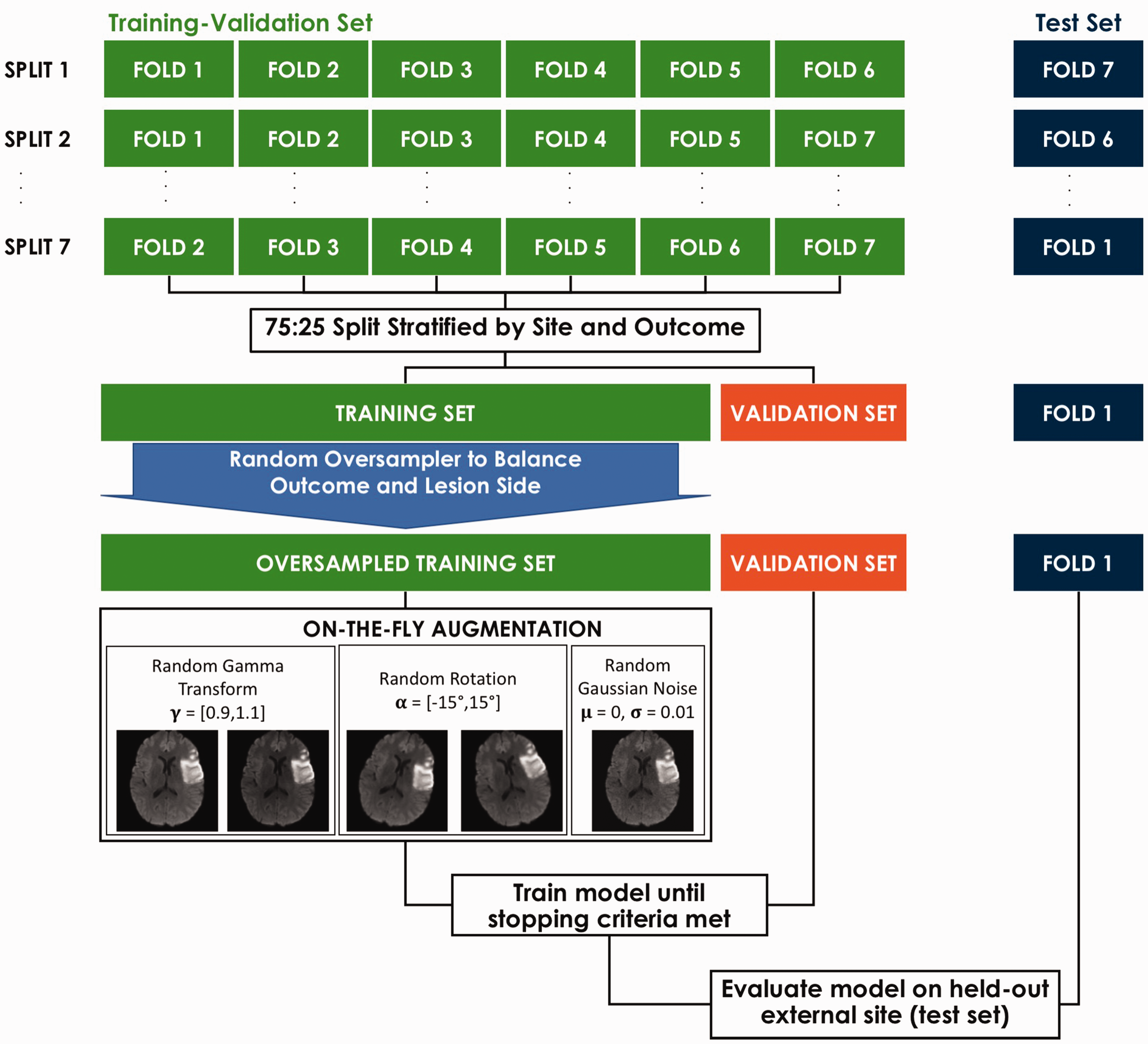
Model training and evaluation scheme. Training and evaluation followed a leave-one-center-out (LOCO) cross-validation scheme.

Trained models were evaluated on images from the held out centers (i.e., test sets). For each fold, independent predictions of the probability of an out-of-center patient having good or poor outcome were obtained. Once all the folds were complete, all out-of-center test set predictions were then merged to form a 322-long prediction vector, the length corresponding to the total number of patients in the study. We computed the unbiased (out of center) accuracy, area under the curve (AUC) from a receiver-operator curve (ROC) analysis, sensitivity, specificity, positive predictive value (PPV), and negative predictive value (NPV) on this vector, instead of averaging the results of each fold. We opted for this approach since the simple average across folds cannot take into account the variable number of patients per center.²³ We calculated 95% confidence intervals (CI) through bootstrapping the merged prediction vector with 10,000 iterations. The run time for test predictions for model inference was recorded. Deep learning model construction and training was carried out on a NVIDIA Quadro RTX 8000 GPU with Tensorflow 2.2.0 in Python 3.8.5.

Comparison to reference imaging biomarkers

We tested the superiority of our deep learning approach against two reference univariate logistic regression models, one using using lesion volume and the other using ASPECTS, which are common biomarkers for predicting functional outcome in clinical trials.^2,12,24,25 Both ASPECTS and lesion volume (manually segmented on the DWI images) were calculated by a trained neurologist with over 15 years of experience (CR) and blind to patient outcome. The logistic regression models were trained and evaluated using the same LOCO cross-validation paradigm using scikit-learn 0.24.1. The AUC of each logistic regression classifier was compared to the most accurate deep learning model with the DeLong test. In addition, we set the probability threshold of the logistic regression classifiers to the specificity of the most accurate deep learning model in order to compare differences in sensitivity with the McNemar test.

Analysis of the attention maps

Since the attention mechanism highlights areas of the image crucial for classification, we sought to inspect model interpretability by visualizing attention throughout the brain in relation to lesion location over the cohort. For each patient in the test set, we extracted the attention maps from all of the 8 light-weight models and projected them back onto the original MRI volume. We then brought all attention maps to MNI space by applying the deformation field estimated from normalizing the b = 0s/mm² image to the MNI T2 template with the Advanced Normalization Tools (ANTs) package.²⁶ We then calculated average attention maps using the normalized attention maps of all patients and all models. To compare the distribution of lesions of the cohort and the attention maps, binary lesion masks were normalized to MNI space by applying the same deformation field as to the attention maps.

We first computed the voxel-wise average attention map per scale (a₁, a₂, a₃) and lesion side (left, right) for all cases. Lesion probability maps were obtained by taking the voxel-wise average of all normalized lesion masks separately for left and right lesions. Second, to better understand the roles that attention and lesion location played for correctly vs. incorrectly predicted cases and for good vs. poor outcome, we re-computed the same average attention maps and lesion probability maps per classification group (i.e., true positives, false positives, false negatives, and true negatives).

Results

Patient population

In total, 322 patients were included in the analysis: 113 patients from the Pitié-Salpêtrière registry, 94 patients from the INSULINFARCT trial, and 115 patients across six centers from the ASTER trial (see Online-Only Data Supplement, Supplemental Figure 2). No differences between the baseline characteristics were detected at admission for age, sex, baseline NIHSS), except for stroke to needle time (p = 0.008) and side of stroke (p < 0.001) (Table 1). There was an overall difference in time to MRI (p = 0.02) driven by longer delays in the INSULINFARCT vs ASTER cohorts (p = 0.01). Overall, almost all patients received a reperfusion treatment (95.3%, n = 307) within 6 hours and 135 (41.9%) had poor outcome. There were no significant differences between baseline characteristics of included or excluded patients except in the Pitié-Salpêtrière registry where excluded patients were older than included ones (p = 0.02, Online-Only Data Supplement, Supplemental Table 2). Lesions followed the typical distribution of middle cerebral artery (MCA) stroke and impacted most commonly the putamen and external capsule for both left (57%) and right (53%) stroke (Figure 2). Lesions from the INSULINFARCT and ASTER trials were similar in volume (p = 0.4) yet significantly larger than those from the Pitié-Salpêtrière cohort (p < 0.001). ASPECTS were comparable across all cohorts (p = 0.4).

Table 1.

Cohort characteristics.

	Overall N = 322	INSULINFARCTN = 94	PS registryN = 113	ASTERN = 115	p-value
Age (years)	68 ± 16	68 ± 16	69 ± 16	68 ± 14	0.882
Female % (n/N)	42.5% (137/322)	38.3% (58/93)	45.1% (58/108)	43.5% (66/111)	0.593
Left Stroke % (n/N)	53.1% (171/322)	47.9% (45/94)	68.1% (77/113)	42.6% (49/115)	<0.001
NIHSS on Admission	15 [8.8–20]	14 [9–19.5]	12.5 [7–20]	16 [10–20]	0.32
Day 1 NIHSS	7 [3–16]	11 [5–17]	5 [2–14]	7 [2–15]	0.002
Stroke-to-needle time (min)	196 ± 104	177 ± 50	186 ± 142	220 ± 81	0.008
Time to MRI (hours)	27.00 [24.00–31.30]	29.30 [26.37–33.95]	28.00 [24.40–31.48]	26.20 [24.00–28.10]	0.02
rtPA % (n/N)	82.9% (266/321)	84.9% (79/93)	100% (113/113)	71.2% (79/111)	<0.001
EVT % (n/N)	32.6% (105/322)	0% (0/94)	31.6% (37/113)	100% (68/115)	<0.001
ASPECTS	6.22 ± 2.59	5.93 ± 2.78	6.48 ± 2.70	6.28 ± 2.31	0.366
Lesion Volume (cc)	27.00 [7.30–78.13]	37.88 [8.35–102.03]	15.03 [4.46–56.81]	31.99 [13.52–82.53]	<0.001
mRS > 2 % (n/N)	41.9% (135/322)	51.1% (48/94)	38.1% (43/113)	38.2% (44/115)	0.10

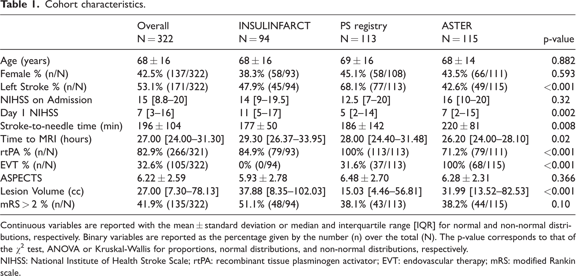
Continuous variables are reported with the mean ± standard deviation or median and interquartile range [IQR] for normal and non-normal distributions, respectively. Binary variables are reported as the percentage given by the number (n) over the total (N). The p-value corresponds to that of the χ² test, ANOVA or Kruskal-Wallis for proportions, normal distributions, and non-normal distributions, respectively.

NIHSS: National Institute of Health Stroke Scale; rtPA: recombinant tissue plasminogen activator; EVT: endovascular therapy; mRS: modified Rankin scale.

Figure 2.

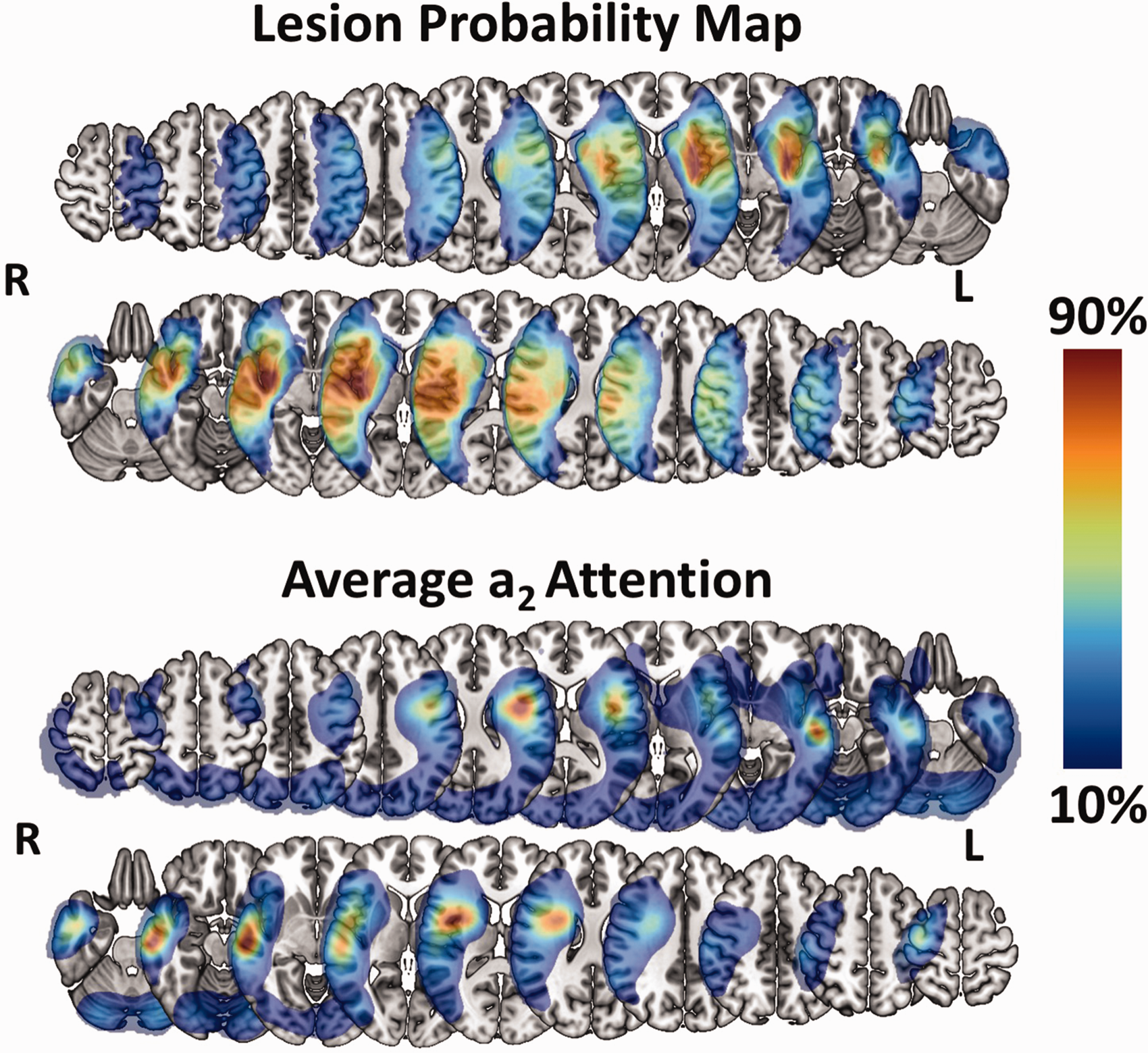
Visual comparison of group-level lesion probability and Model a₂ attention. Lesion probability map and average a₂ attention. For each map, lesion probability and attention are shown on separate rows for patients with left-sided (top) and right-sided (bottom). The average attention is taken over all deep learning models. Selected slices are located at the following z coordinates in MNI space in mm: –26, –16, –6, 4, 14, 24, 24, 34, 44, 54, 64. L = Left, R = Right. Colorbar reflects the percentage of the maximum value of both the attention and lesion probability maps.

Classification performance

With respect to deep learning, the eight individual models trained similarly on all folds with some overfitting on the training set (see Online-Only Data Supplement, Supplemental Figure 3). All models performed comparably on the external test sets with the deep learning ensemble model attaining the highest accuracy of 0.79 [0.74–0.83], highest AUC of 0.83 [0.78–0.87], the tied for third best sensitivity of 0.67 [0.59–0.73], second best specificity of 0.87 [0.82–0.92], the best PPV of 0.79 [0.71–0.86], and the best NPV of 0.78 [0.73–0.84] (Table 2, Online-Only Data Supplement, Supplemental Table 3). The average run time of a patient to go through all 8 models for ensemble model inference was 0.46 ± 0.31 seconds with GPU acceleration and only slightly slower on a CPU at 0.60 ± 0.30 seconds.

Table 2.

Classification performance.

Model	Accuracy	AUC	Sensitivity	Specificity	PPV	NPV
LR – Lesion Volume	0.71 [0.66–0.76]	0.78 [0.73–0.83]	0.48 [0.40–0.56]	0.87 [0.82–0.92]	0.73 [0.64–0.82]	0.70 [0.64–0.76]
LR – ASPECTS	0.70 [0.65–0.76]	0.77 [0.71–0.82]	0.56 [0.47–0.65]	0.82 [0.76–0.88]	0.71 [0.61–0.79]	0.70 [0.63–0.77]
LR – ASPECTS^a	0.70 [0.64–0.75]	0.77 [0.71–0.82]	0.50 [0.41–0.58]	0.87 [0.84–0.93]	0.76 [0.66–0.85]	0.68 [0.61–0.74]
Deep learning ensemble	0.79 [0.74–0.83]	0.83 [0.78–0.87]	0.67 [0.59–0.75]	0.87 [0.82–0.92]	0.79 [0.71–0.86]	0.78 [0.73–0.84]

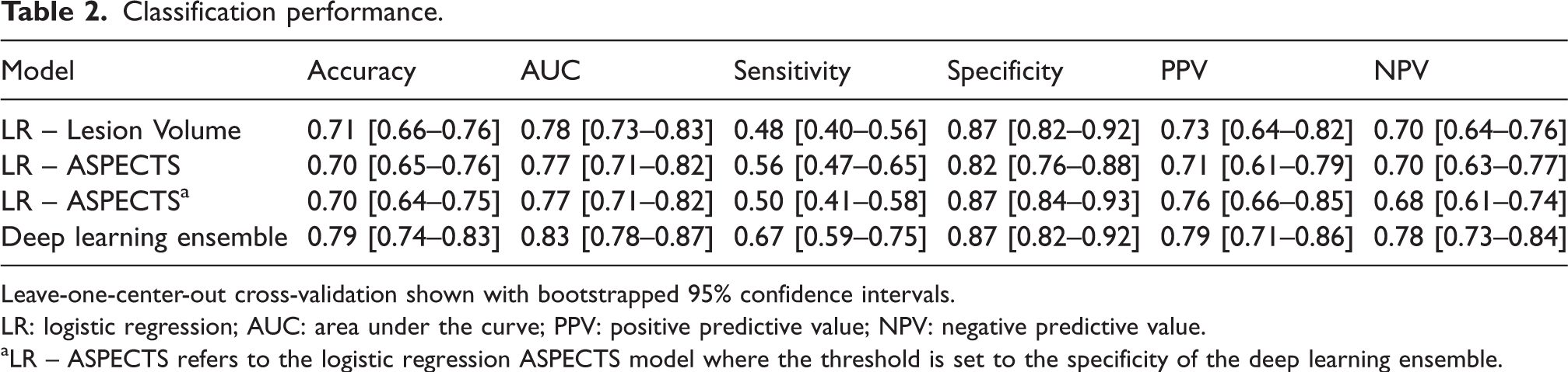
Leave-one-center-out cross-validation shown with bootstrapped 95% confidence intervals.

LR: logistic regression; AUC: area under the curve; PPV: positive predictive value; NPV: negative predictive value.

^aLR – ASPECTS refers to the logistic regression ASPECTS model where the threshold is set to the specificity of the deep learning ensemble.

The logistic regression model with lesion volume yielded an accuracy of 0.71 [0.66–0.76], AUC of 0.78 [0.73–0.83], sensitivity of 0.48 [0.40–0.56], specificity of 0.87 [0.82–0.92], a PPV of 0.73 [0.64–0.82], and a NPV of 0.70 [0.64–0.76] with a median cut–off value of 70.11 cc [69.44–72.44]. The logistic model with ASPECTS yielded an accuracy of 0.70 [0.65–0.76], AUC of 0.77 [0.71–0.82], a sensitivity of 0.56 [0.47–0.65], specificity of 0.82 [0.76–0.88], a PPV of 0.71 [0.61–0.79], and a NPV of 0.70 [0.63–0.77] with median cut-off value of 5.79 [5.66–5.82]. After setting the thresholds of the logistic regression classifiers to the specificity as the deep learning ensemble model, and ASPECTS yielded an accuracy of 0.70 [0.64–0.75], sensitivity of 0.50 [0.41–0.58], PPV of 0.76 [0.66–0.85], and NPV of 0.68 [0.61–0.74].

The deep learning ensemble model had a significantly higher AUC than lesion volume (p = 0.04) and ASPECTS (p = 0.008). With specificities fixed to 0.87, the deep learning ensemble had significantly higher sensitivity than both lesion volume (p = 0.002) and ASPECTS (p = 0.002) (Figure 3).

Figure 3.

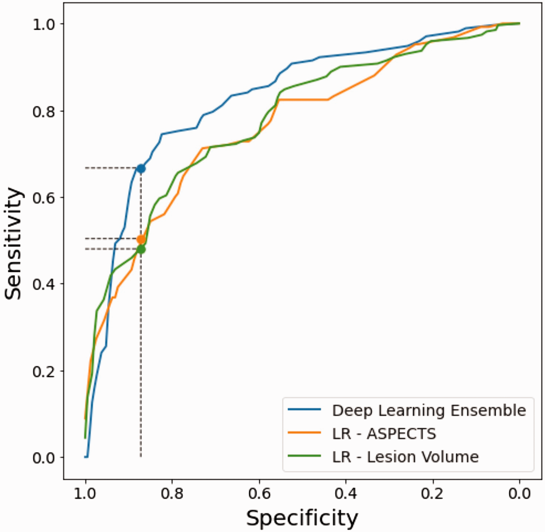
Receiver-operator characteristic (ROC) curves. ROC curves for the deep learning ensemble model (blue), logistic regression (LR) ASPECTS (orange), and LR Lesion Volume (green). The vertical line corresponds to the specificity of the deep learning ensemble model and highlights the significant gain in sensitivity of the deep learning ensemble model of +0.19 and +0.17 with respect to the LR ASPECTS and LR Lesion Volume classifiers, respectively.

Model attention and lesion distribution

Model attention on was largely localized to the affected hemisphere and was comparable for left- and right-sided lesions (Figure 2). As we expected, the model attention focused on and heavily coincided with lesioned areas of the brain at both the group (Figure 2) and individual (Figure 4) levels. For illustrative purposes, only the average a₂ attention is shown in the main text since this level constitutes the best compromise of spatial specificity. Examples of a₁ and a₃ attention maps at the group and individual levels are provided in Online-Only Data Supplement Supplemental Figures 4 and 5, respectively.

Figure 4.

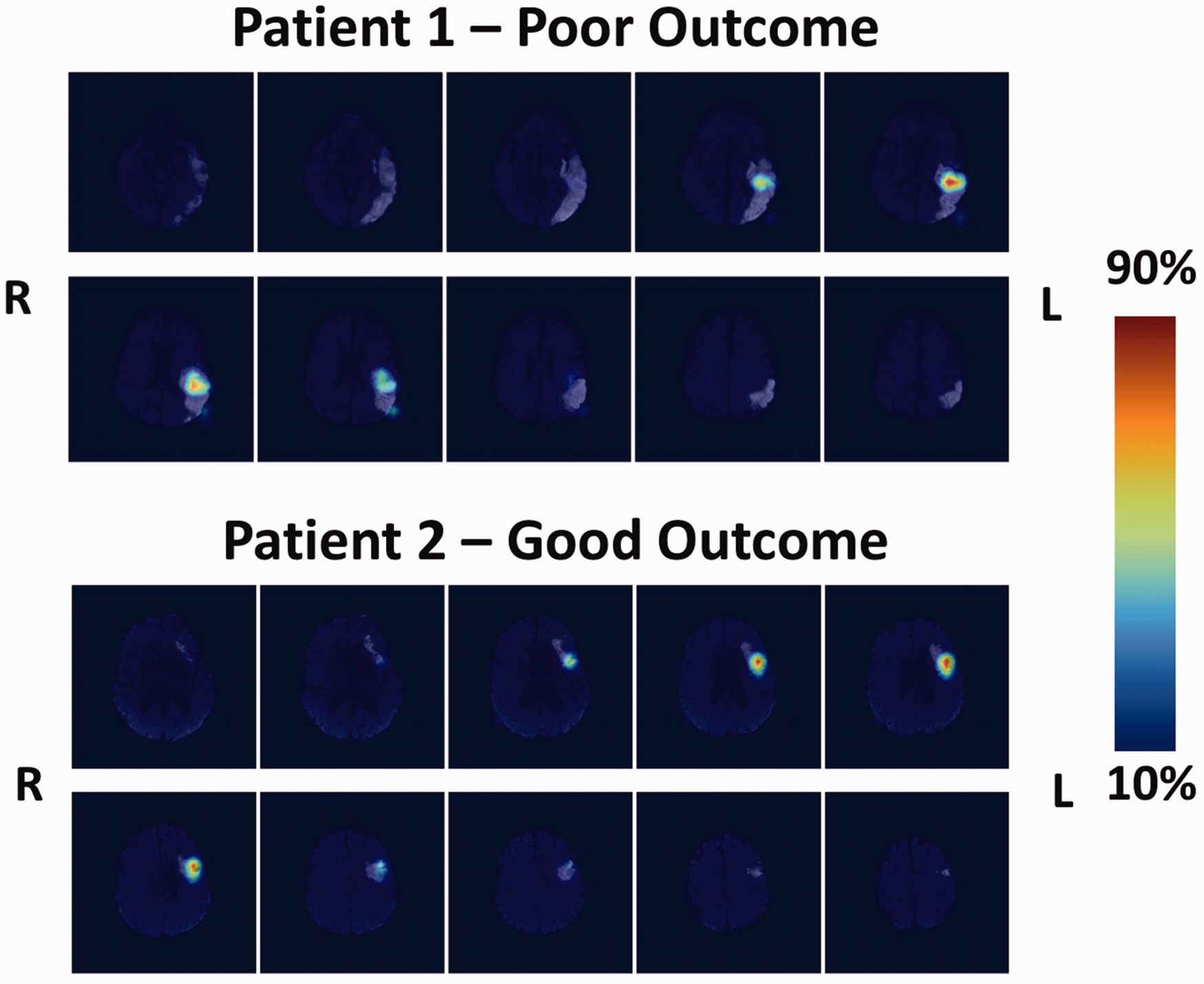
Individual attention maps. Patient 1 (top): Patient, 82 yo, admitted to the hospital for a left MCA territory ischemic lesion with a baseline NIHSS of 12. He had a delayed reperfusion treatment (stroke-to-groin puncture time: 340 minutes), which led to an incomplete recanalization and clinical worsening (Day 1 NIHSS: 14). At 3 months, his mRS was 3. The ensemble model correctly predicted this case with an average attention map over all models highlighting the lesioned temporo-parietal junction, a region known to be crucial for aphasia recovery. Patient 2 (bottom): Patient, 71 yo, admitted to the hospital for a left MCA territory ischemic lesion with a baseline NIHSS of 10. She received thrombolysis with a stroke-to-needle time of 221 minutes. Recanalization was complete and her day one NIHSS was 9. Her mRS at 3 months was 2. The ensemble model correctly predicted this case with an average attention map over all models highlighting a lesioned Broca's area and premotor cortex. Colorbar reflects the percentage of the maximum value of each attention map.

Regarding the lesion probability and average attention maps per classification group (i.e., true positives, false positives, false negatives, true negatives), attention remained concordant with the lesion distribution for both good and poor outcome (Figure 5, see Online-Only Data Supplement, Supplemental Figure 6). The only exception was for a₃ attention where there seemed to be a larger mix of attention on lesioned and non-lesioned areas that live along a gradient of true negatives, false negatives, false positives, and true positives. In other words, as we move from true negatives to false negatives, false positives, and true positives, the systematic attention to lesion-inconsistent regions becomes gradually less strong and is ultimately replaced by strong attention exclusively over the lesions.

Figure 5.

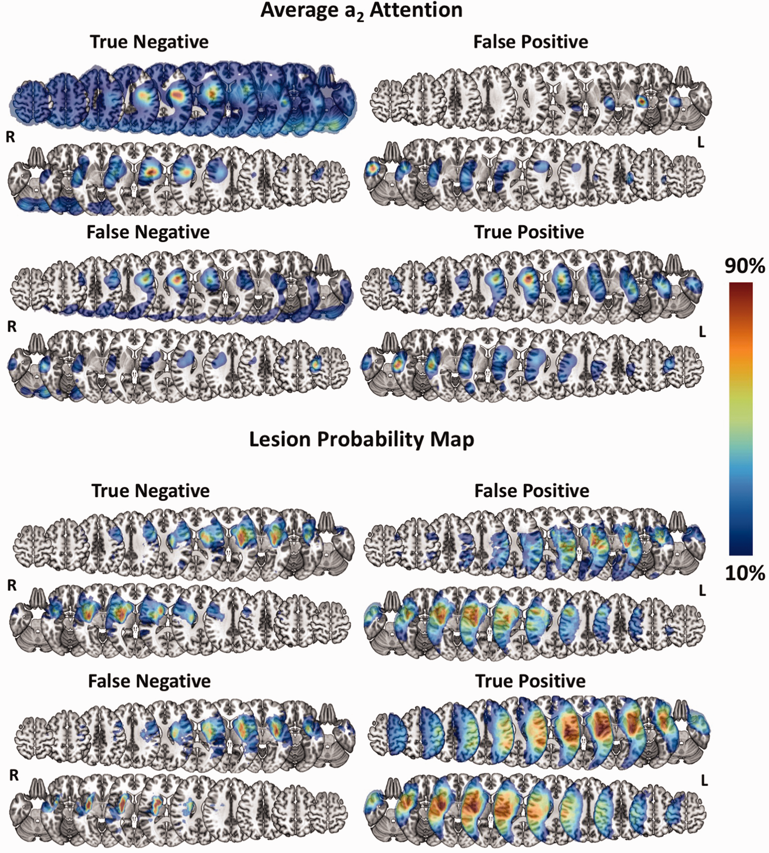
Visual comparison of group-level lesion probability and Model a₂ attention per classification group. Top: Average a₂ attention per classification group. Colorbar reflects the percentage of the maximum attention value per map and side to highlight the areas to which the model attributed the most attention. Bottom: Lesion probability map per classification group. Colorbar reflects the percentage of the maximum lesion probability per map and side. For each group, lesion probability and attention are shown on separate rows for patients with left-sided (top row) and right-sided (bottom row) lesions. The average attention is taken over all deep learning models. Selected slices are located at the following z coordinates in MNI space in mm: –26, –16, –6, 4, 14, 24, 24, 34, 44, 54, 64. L = Left, R = Right.

Discussion

Using day 1 DWI data from three cohorts with different imaging protocols, we built a robust deep learning CNN model to predict 3-month long-term functional outcome with good accuracy. Moreover, we have shown that our model highly attends to lesioned areas of the brain to generate both poor and good outcome predictions, all while performing significantly more accurately than the traditionally used biomarkers, lesion volume and ASPECTS.

Classification performance comparison to previous studies

Our study presents several methodological advantages over previous studies. First, similar existing studies have confounded the link between early stroke topography and long-term outcome by using pre-reperfusion treatment images to train CNN models. However, depending on its success, reperfusion therapy can drastically change the final extent of the infarct and thus have a substantial effect on the trajectory of recovery.^12,13 In our study, we used day 1 DWI images, when the effects of hyper-acute reperfusion therapy on lesion size are clearly seen.^13,15 This difference in methodology likely contributes to the superior performance of our model with respect to existing studies since the variability in infarct growth is no longer a present factor in our cohort. Here, we report a high out-of-center external validation accuracy of 0.79 and AUC of 0.83 with a marginally unbalanced dataset (41.9% poor outcome), albeit representative of cohorts in other endovascular therapy and thrombolysis studies. On the other hand, of the pure imaging models for predicting poor outcome (defined as mRS > 2) with CNNs, two studies reported external validation accuracies of 0.65¹¹ and 0.75⁸, while one only reported an area under the curve of 0.71⁹. Of note, the study reporting an accuracy of 0.75 was based on a cohort with 75% of poor outcome, rendering their model no better than a majority class classifier. Another study using an alternative cutoff of mRS > 1 for poor outcome reported an accuracy of 0.65⁷.

A second advantage of our study is the leave-one-center-out cross-validation paradigm. We used DWI data from eight hospitals, each with different imaging protocols, and always held out data from one center to obtain a completely unbiased measure of model performance. The rich, diverse data used for training likely enabled a meaningful extraction of features related more to stroke outcome and less to the specific centers from which the data originated. In fact, there was no evidence that a specific site drove the accuracy across folds despite the highly variable number of patients over centers and some differences in baseline demographics (see Online-Only Data Supplement, Supplemental Table 4). This ultimately resulted in an external test accuracy and AUC not only higher than in previous studies but also more reliable. Indeed, previous studies have used either a random split of all data for training and test data^7–9 or used a single set of held-out centers for external validation.¹¹ We opted for multiple held-out centers for external validation to not only reduce the variance on our estimated classification performance but also to simulate its performance on unseen data from multiple, new hospitals.

The importance of lesion topography for prognosis

In order for deep learning solutions to earn the trust of clinicians, their predictions need to be explainable. A common method of doing so with CNNs is to demonstrate that the model attends to anatomical features related to the clinical question at hand.^9,11,27 In our case, the lesion consistently proved to be a crucial area for generating predictions for poor outcome, corroborating the repeatedly demonstrated link between infarct topology and functional outcome in the literature.^1,4,28–33 It is also interesting to speculate on the significance of the attention maps at each level and how they relate to lesion topology. First, the feature maps at the a₁ attention level operate at an early stage in the network and are thus more fine-tuned to sharp changes in contrast (i.e., edges) and texture. For this reason, the a₁ map is mostly focused on small lesions or at the intersection of larger lesions and healthy tissue (Supplemental Figure 6). The presumed focus of a₁ on the cortex is likely explained by the fact that, on a population level, the highest lesion overlap coincidentally occurs along the cortical ribbon of the insula and the lateral face of the brain in addition to the basal ganglia. As we move down in the network, the convolutional layers respond to larger receptive fields and can thus activate for lesions covering a larger area. This is why the average attention at levels a₂ and a₃ are larger and coincide more with the whole average spatial extent of the lesions. While each attention map is sensitive to different aspects of the lesion and at different spatial scales, the network ultimately requires all three attention maps to drive proper classification; therefore, all attention maps are necessary and clinically relevant.

In fact, our model highly attended to lesioned areas of the brain when predicting poor outcome or good outcome (see Online-Only Data Supplement, Supplemental Figures 5 and 6). The only exception was for a₃ attention where there was a gradual shift from attention on non-lesioned areas for true negatives to lesion-exclusive attention for true positives. This phenomenon may have arisen from how the network came to encode good outcome despite a present lesion. More precisely, in order to predict good outcome, we speculate that the network may have deliberately learned to attend to consistently non-lesioned iso-signal areas at the a₃ level in order to suppress strong attention on hyper-signal lesioned areas at the a₁ and a₂ levels, which could have otherwise pushed the model’s prediction towards poor outcome. This can explain the observed gradient at the a₃ level (from true negatives to false negatives, false positives, and true positives) of attention to lesion-inconsistent to exclusively lesion-consistent regions.

Interestingly, the model often did not attend to the whole lesion but specific parts of it. For example, the true positive case in Figure 4 shows a patient with a large left lesion extending from the temporal lobe superiorly to the precentral gyrus. However, attention was highest on the underlying white matter of the temporo-parietal junction where the arcuate fasciculus arches around the Sylvian fissure. This infarcted area was likely responsible for severe aphasia, resulting in dependence on external aid at 3 months post-stroke for this patient.³⁴ This finding also applied to the group level where the average attention maps for the true positive cases were less extensive than the large lesion distribution for the same group, supporting the notion that lesion location is more important than the size of the entire lesion.¹³ In fact, since our model had access to the entire MRI volume, it was likely able to learn and extract rich features about lesion location and size, which crude measurements like lesion volume and ASPECTS are not able to encode well. This may explain our model’s superior prognostic value than these traditional biomarkers. Specifically regarding lesion volume, a post-hoc analysis revealed that the deep learning and lesion volume classifiers had similar performance for both small (<5 cc) and large lesions (>70 cc), but not for medium-sized lesions (5–70 cc) where the deep learning model significantly had a higher rate of better predictions where the lesion volume model failed (p = 0.009, Online-Only Data Supplement, Supplemental Table 5). This result demonstrates that while our deep learning model is able to reproduce correct predictions made by a lesion volume classifier using standard cutoff values for small and large lesions,³⁵ the added value of our model truly lies within the higher rate of correct predictions in the transition range of medium-sized lesions.

Investigators of a similar study employed a post-hoc attention mechanism on a CNN model that was simultaneously trained to segment acute lesions on DWI and predict 3-month functional outcome. Their attention maps also highlighted pathological tissue; however, it was unclear whether the model was biased towards imaging features of the lesion, since the model was jointly trained for lesion segmentation. In our case, we trained our model to directly predict long-term outcome from DWIs, and the CNN naturally learned to attend to lesion-related features without any a priori transfer learning or contemporaneous multi-task learning,³⁶ strengthening the relation between the lesion and outcomes.

Limitations

Despite our promising results, our study presents some limitations. First, deep learning algorithms require large volumes of data in order to generalize properly, especially for stroke due to the great heterogeneity of the disease. In our case, our model performed well on external test sets but was subject to some overfitting likely due to the small number of patients in the cohort. We attempted to mitigate this effect by implementing on-the-fly data augmentation and a low-parameter model. Moreover, our dataset included strokes primarily affecting the MCA territory and could not be extensively trained or evaluated on strokes of other vascular territories. More data would have undoubtedly allowed us to increase model complexity and likely improve predictions on unseen data covering a larger range of stroke types and locations.

Second, this model is based on purely imaging data, yet deep learning has also been shown to effectively harness clinical data, such as age, NIHSS, and pre-stroke mRS, for prognostication.³⁷ Future work should investigate the best ways to combine both imaging and clinical data to improve prognosis, which was beyond the scope of this study. Regardless, image-based models have the benefit of being completely automatable by surpassing the need for manually entered clinical data, making these techniques easier to integrate into patient management strategies. In particular, our model works directly on images in their native space and can generate predictions and attention maps in less than a second, adding almost no extra time to clinical workflow.

Finally, while model attention on the lesion is important for interpretation and instilling trust, it remains difficult to determine precisely what information the model is extracting from the lesion and how the model is manipulating it. At this stage, we can only speculate that the model is able to incorporate information and interactions between lesion size and location to drive better predictions.³⁸ Advances in research on model inspection will help elucidate these unanswered questions in the future.

Conclusion

We developed a robust deep learning CNN to predict long-term functional outcome using DWI on day 1 post-stroke. Our model would be most beneficial as a strategy for patient stratification for neuroprotection and rehabilitation therapies once standard hyper-acute reperfusion treatments have been performed. As the clinical community continues to adopt artificial intelligence solutions into imaging workup, deep learning models such as ours could be deployed in hospital settings to improve patient care and outcome.

Supplemental Material

sj-pdf-1-jcb-10.1177_0271678X221129230 - Supplemental material for Interpretable deep learning for the prognosis of long-term functional outcome post-stroke using acute diffusion weighted imaging

Supplemental material, sj-pdf-1-jcb-10.1177_0271678X221129230 for Interpretable deep learning for the prognosis of long-term functional outcome post-stroke using acute diffusion weighted imaging by Eric Moulton, Romain Valabregue, Michel Piotin, Gaultier Marnat, Suzana Saleme, Bertrand Lapergue, Stephane Lehericy, Frederic Clarencon, Charlotte Rosso in Journal of Cerebral Blood Flow & Metabolism

Footnotes

Funding

The author(s) disclosed receipt of the following financial support for the research, authorship, and/or publication of this article: The ASTER trial was sponsored by the Fondation Ophtalmologique Adolphe de Rothschild. An unrestricted research grant was provided for the ASTER trial by Penumbra, Alameda, California. No grant was provided for this analysis and this study. The research leading to these results has received funding from “Investissements d’avenir” ANR-10-IAIHU-06.

Acknowledgements

The Pitié-Salpêtrière registry was supported by the French Ministry of Health grant EVALUSINV PHRC AOM 03 008.

Declaration of conflicting interests

The author(s) declared no potential conflicts of interest with respect to the research, authorship, and/or publication of this article.

Authors’ contributions

MP, GM, SS, BL, SL, FC made a substantial contribution to the concept and design, acquisition of data or analysis and interpretation of data and approved the version to be published

EM, RV, and CR made a substantial contribution to the concept and design, acquisition of data or analysis and interpretation of data and drafted the article or revised it critically for important intellectual content, and approved the version to be published

EM and CR accept direct responsibility for the manuscript.

ORCID iDs

Eric Moulton

Charlotte Rosso

Supplemental material

Supplemental material for this article is available online.

References

Etherton

Rost

Infarct topography and functional outcomes. J Cereb Blood Flow Metab 2018; 38: 1517–1532.

Barber

Demchuk

Zhang

, et al. Validity and reliability of a quantitative computed tomography score in predicting outcome of hyperacute stroke before thrombolytic therapy. Lancet 2000; 355: 1670–1674.

Yoo

Barak

Copen

, et al. Combining acute diffusion-weighted imaging and mean transmit time lesion volumes with national institutes of health stroke scale score improves the prediction of acute stroke outcome. Stroke 2010; 41: 1728–1735.

Moulton

Valabregue

Lehéricy

, et al. Multivariate prediction of functional outcome using lesion topography characterized by acute diffusion tensor imaging. NeuroImage Clin 2019; 23: 101821.

Corbetta

Ramsey

Callejas

, et al. Common behavioral clusters and subcortical anatomy in stroke. Neuron 2015; 85: 927–941.

Zhang

Wang

Liu

, et al. A survey on deep learning for neuroimaging-based brain disorder analysis. Front Neurosci 2020; 14: 1–19.

Bacchi

Zerner

Oakden-Rayner

, et al. Deep learning in the prediction of ischaemic stroke thrombolysis functional outcomes: a pilot study. Acad Radiol 2020; 27: e19–e23.

Samak

Clatworthy

Mirmehdi

Prediction of thrombectomy functional outcomes using multimodal data. Comput Med Imaging Graph 2022; 99: 102089.

Hilbert

Ramos

van Os

HJA

, et al. Data-efficient deep learning of radiological image data for outcome prediction after endovascular treatment of patients with acute ischemic stroke. Comput Biol Med 2019; 115: 103516.

10.

Choi

Kwon

Lee

, et al. Ensemble of deep convolutional neural networks for prognosis of ischemic stroke. Berlin Germany: Springer Verlag, 2016, pp.231–243.

11.

Nishi

Oishi

Ishii

, et al. Deep learning-derived high-level neuroimaging features predict clinical outcomes for large vessel occlusion. Stroke 2020; 51: 1484–1492.

12.

Rosso

Corvol

Pires

, et al. Intensive versus subcutaneous insulin in patients with hyperacute stroke: results from the randomized INSULINFARCT trial. Stroke 2012; 43: 2343–2349.

13.

Rosso

Samson

The ischemic penumbra: the location rather than the volume of recovery determines outcome. Curr Opin Neurol 2014; 27: 35–41.

14.

Lapergue

Blanc

Gory

, et al. Effect of endovascular contact aspiration vs stent retriever on revascularization in patients with acute ischemic stroke and large vessel occlusion. JAMA 2017; 318: 443–452.

15.

Rosso

Blanc

, et al. Impact of infarct location on functional outcome following endovascular therapy for stroke. J Neurol Neurosurg Psychiatry 2019; 90: 313–319.

16.

Quinn

Singh

Lees

, et al. Validating and comparing stroke prognosis scales. Neurology 2017; 89: 997–1002.

17.

Jenkinson

Pechaud

Smith

BET2-MR-based estimation of brain, skull and scalp surfaces. Hum Brain Mapp 2002; 17: 143–155.

18.

Jetley

Lord

Lee

, et al. Learn to pay attention. arXiv. 2018. arXiv:1804.02391.

19.

Simonyan

Zisserman

Very deep convolutional networks for large-scale image recognition. 3rd Int Conf Learn Represent ICLR 2015 – Conf Track Proc 2014; 1–14. https://arxiv.org/abs/1409.1556.

20.

Celaya

Actor

Muthusivarajan

, et al. PocketNet: a smaller neural network for medical image analysis.

21.

Kotu

Deshpande

Data mining process. In: Predictive analytics and data mining. The Netherlands: Elsevier, 2015, pp.17–36.

22.

Winzeck

Giese

, et al. Big data approaches to phenotyping acute ischemic stroke using automated lesion segmentation of multi-center magnetic resonance imaging data. Stroke 2019; 50: 1734–1741.

23.

Betancur

Commandeur

, et al. Deep learning analysis of upright-supine high-efficiency SPECT myocardial perfusion imaging for prediction of obstructive coronary artery disease: a multicenter study. J Nucl Med 2019; 60: 664–670.

24.

Nogueira

Jadhav

Haussen

, et al. Thrombectomy 6 to 24 hours after stroke with a mismatch between deficit and infarct. N Engl J Med 2018; 378: 11–21.

25.

Albers

Marks

Kemp

, et al. Thrombectomy for stroke at 6 to 16 hours with selection by perfusion imaging. N Engl J Med 2018; 378: 708–718.

26.

Avants

Epstein

Grossman

, et al. Symmetric diffeomorphic image registration with cross-correlation: evaluating automated labeling of elderly and neurodegenerative brain. Med Image Anal 2008; 12: 26–41.

27.

Lee

Yune

Mansouri

, et al. An explainable deep-learning algorithm for the detection of acute intracranial haemorrhage from small datasets. Nat Biomed Eng 2019; 3: 173–182.

28.

Cheng

Forkert

Zavaglia

, et al. Influence of stroke infarct location on functional outcome measured by the modified Rankin scale. Stroke 2014; 45: 1695–1702.

29.

Munsch

Sagnier

Asselineau

, et al. Stroke location is an independent predictor of cognitive outcome. Stroke 2016; 47: 66–73.

30.

Cloonan

Mocking

SJT

, et al. Role of acute lesion topography in initial ischemic stroke severity and long-term functional outcomes. Stroke 2015; 46: 2438–2444.

31.

Rosso

Colliot

Pires

, et al. Early ADC changes in motor structures predict outcome of acute stroke better than lesion volume. J Neuroradiol 2011; 38: 105–112.

32.

Cuingnet

Rosso

Chupin

, et al. Spatial regularization of SVM for the detection of diffusion alterations associated with stroke outcome. Med Image Anal 2011; 15: 729–737.

33.

Payabvash

Taleb

Benson

, et al. Acute ischemic stroke infarct topology : association with and discharge. Am J Neuroradiol 2017; 58–63.

34.

Moulton

Magno

Valabregue

, et al. Acute diffusivity biomarkers for prediction of motor and language outcome in mild-to-severe stroke patients. Stroke 2019; 50: 2050–2056.

35.

Yoo

Verduzco

Schaefer

, et al. MRI-based selection for intra-arterial stroke therapy: value of pretreatment diffusion-weighted imaging lesion volume in selecting patients with acute stroke who will benefit from early recanalization. Stroke 2009; 40: 2046–2054.

36.

Tian

Fang

Dong

, et al. Using multi-task learning to improve diagnostic performance of convolutional neural networks. In: Hahn

Mori

(eds) Medical imaging 2019: computer-aided diagnosis, p. 67. SPIE, 2019. doi: 10.1117/12.2512153.

37.

Heo

Yoon

Park

, et al. Machine learning-based model for prediction of outcomes in acute stroke. Stroke 2019; 50: 1263–1265.

38.

Benghanem

Rosso

Arbizu

, et al. Aphasia outcome: the interactions between initial severity, lesion size and location. J Neurol 2019; 266: 1303–1309.

Supplementary Material

Please find the following supplemental material available below.

For Open Access articles published under a Creative Commons License, all supplemental material carries the same license as the article it is associated with.

For non-Open Access articles published, all supplemental material carries a non-exclusive license, and permission requests for re-use of supplemental material or any part of supplemental material shall be sent directly to the copyright owner as specified in the copyright notice associated with the article.

0.00 MB

1.89 MB