Sage Journals: Discover world-class research

Abstract

Full kinetic modeling of dynamic PET images requires the measurement of radioligand concentrations in the arterial plasma. The unchanged parent radioligand must, however, be separated from its radiometabolites by chromatographic methods. Thus, only few samples can usually be analyzed and the resulting measurements are often noisy. Therefore, the measurements must be fitted with a mathematical model. This work presents a comprehensive analysis of the different models proposed in the literature to describe the plasma parent fraction (PPf) and of the alternative approaches for radiometabolite correction. Finally, we used a dataset of [¹¹C]PBR28 brain PET data as a case study to guide the reader through the PPf model selection process.

Keywords

PET plasma parent fraction radiometabolite correction PPf modeling

Introduction

The accurate measurement of parent radioligand concentration in plasma is a major challenge of quantitative PET imaging. Radiolabeled compounds injected into the blood stream are exposed to a complex and unpredictable chemical environment and thus may break down in one or more metabolites. At least one of these metabolites would contain the radioisotope and is therefore named radiometabolite. To correctly quantify the binding of a radioligand, the amount of radiometabolites should be taken into account.¹

Depending on the chemical characteristics of the radiometabolites and on the transport mechanism between blood and tissue, the radiometabolites may remain confined to the vascular compartment, migrate into the tissue along with the parent radioligand or even be created inside the tissue. Radiometabolites are often less lipophilic than their parent, and therefore are less likely to cross the blood–brain barrier and enter the brain. Thus, if the radiometabolites are confined to the blood compartment, only the concentration of parent radioligand should be used as input for modeling the tissue kinetics. By contrast, radiometabolites that cross the blood–brain barrier or originate directly inside the tissue² must be incorporated into the model as a second input or as an additional compartment, respectively.

Serial arterial blood samples are usually drawn during the PET scan, in order to assess the concentration of parent radioligand over time. Blood samples may be drawn manually or with an automated blood sampling system equipped with an online detector or with a fraction collector. The online detector allows the best definition of the peak, by continuously measuring arterial whole-blood concentrations. However, some manual blood samples are still required to obtain the plasma concentration and to separate the parent from its radiometabolites. The fraction collector instead provides discrete blood measurements as in the manual sampling, but with a higher frequency and more precise timing.

The fraction of unchanged radioligand in plasma (the Plasma Parent fraction or PPf) is measured with techniques such as high-performance liquid chromatography (HPLC), thin layer chromatography or other chromatographic methods. The fast decay of radioactivity, especially with ¹¹C-labeled tracer, limits the total number of samples that can be analyzed by chromatography. Therefore, for kinetic modeling, PPf data points are generally fitted with a mathematical function, with the purpose of obtaining a smooth and continuous PPf curve from a series of discrete noisy samples. Although PPf measurements are sometimes linearly interpolated,^3,4 the use of a model is preferable to minimize the impact of measurement errors.⁵ The choice of the PPf model is a crucial step for kinetic modeling. Indeed, a carefully selected PPf model allowed Parsey and colleagues⁶ to nearly halve the retest variability of the total volume of distribution (V_T) of [¹¹C]DASB compared to the results obtained with the PPf model commonly used in the literature. Furthermore, Wu et al.⁷ showed that different models can lead to significant differences in both binding potential ( $BP$ ) and V_T quantification of [¹¹C]WAY-100635.

The aims of this review are 1) to overview the most common modeling approaches to correct the plasma input function for radiometabolites and 2) to define guidelines for selecting the optimal PPf model. A dataset of 11 brain PET studies done with [¹¹C]PBR28, a radioligand for the translocator protein, is used as a case study. The approaches developed to obtain a full input function from a limited number of blood samples are discussed in detail. Finally, we will outline some alternative modeling strategies for radiometabolite correction.

Plasma parent fraction modeling

Obtaining a radiometabolite-corrected arterial input function is a multistep procedure (Figure 1) that usually involves:

Measurement of the whole blood activity – $C_{b} (t)$ .

Separation of plasma from whole blood by centrifugation and measurement of the total activity in plasma – $C_{tot} (t)$ .

Analysis of plasma samples by chromatographic methods to determine the fraction of activity that is due to the parent tracer – $PPf (t)$ .

Figure 1.

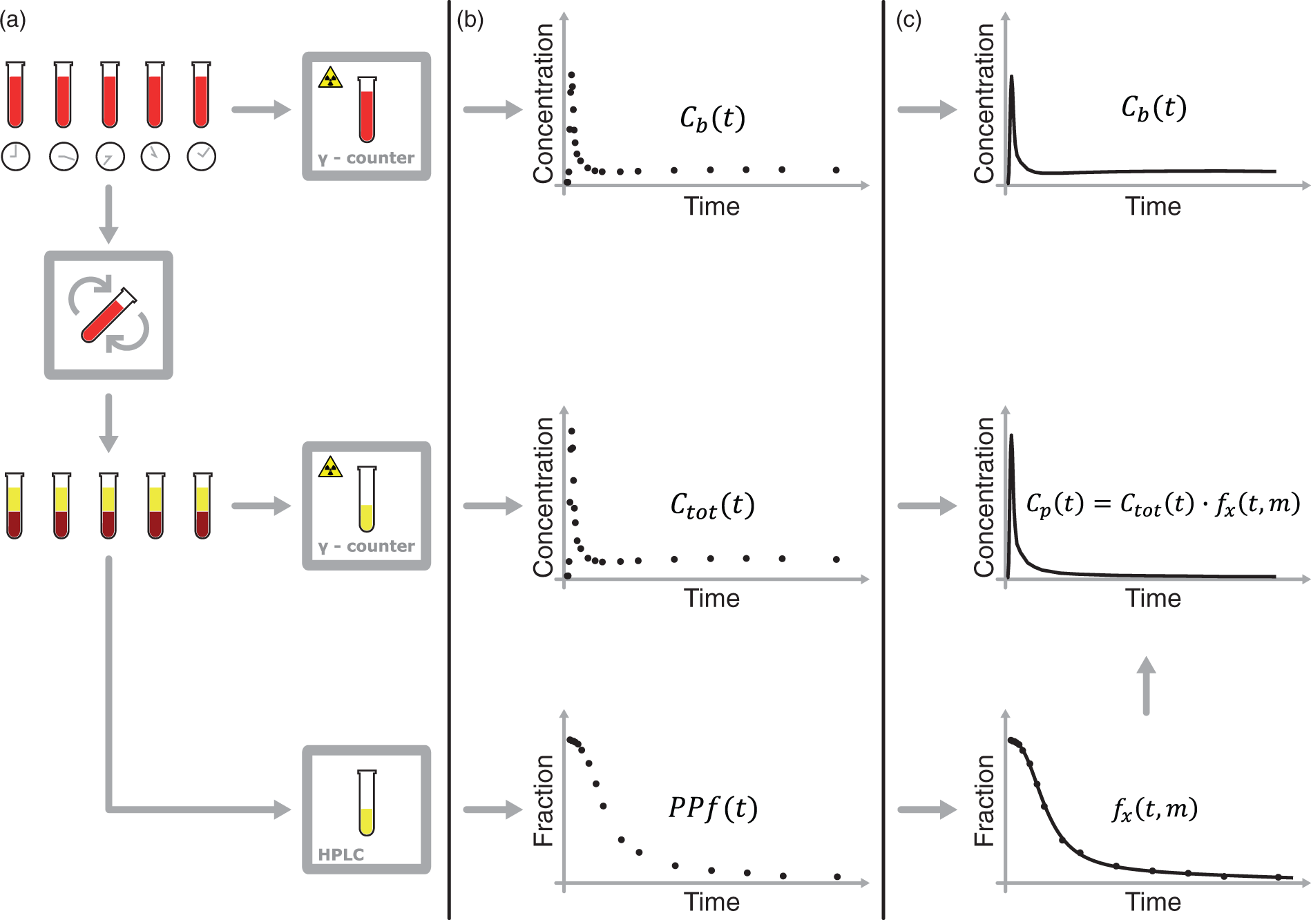
Blood samples processing for the derivation of the input function. (a) Blood samples are drawn at various time points and their radioactivity is measured with a γ-counter. The samples are then centrifuged to separate the blood cells from plasma (b) The whole blood activity – $C_{b} (t)$ – and the total activity in plasma – $C_{tot} (t)$ – are measured with the γ-counter. The HPLC measures the fraction of activity due to the parent in plasma – $PPf (t)$ . (c) $C_{b} (t)$ can be used either after linear interpolation or after fitting with an appropriate model. Although PPf data can be used after linear interpolation, they are more usually fitted with a tracer specific model – $f_{x} (t, m)$ – where x identifies the specific radiotracer and m is the vector of the estimated parameters. The input function is calculated as $C_{p} (t) = C_{tot} (t) \cdot f_{x} (t, m)$ .

Because of their limited number and the presence of noise in the measurements, PPf data points are rarely used directly. A PPf model is generally fitted to the data in order to extrapolate the missing values and to minimize the impact of measurement errors. The parent concentration in plasma is calculated as

C_{p} (t) = C_{tot} (t) \cdot f_{x} (t, m)

(1)

where

f_{x} (t, m)

is the PPf model of the radiotracer x and

m

is the vector of parameters estimated from

PPf (t)

. The model

f_{x} (t, m)

reflects the PPf properties: its value may range from 1 to 0, where 1 means that all radioactivity measured from the plasma sample is due to the unchanged radioligand and 0 that the radioligand has been completely metabolized.

The PPf curve has usually an initial value of 1 and then decreases monotonically and sigmoidally toward 0. However, different shapes are possible. For example, the parent fraction of [¹¹C]DASB displays an initial rising phase,⁶ probably because the parent, but not the radiometabolites, is trapped in the lungs. The majority of PPf models can be categorized into three main classes: Power models, Hill models and Exponential models (Table 1).⁸

Table 1.

Plasma Parent fraction models used in the literature.

Tracer	Equation	References
Power model
[¹¹C]MDL 100,907 [¹¹C]MPDX	$[1 + (at)^{2}]^{- b}$	⁹ ¹⁰
[¹⁸F]CPFPX	${1, t \leq t_{0} [1 + (a (t - t_{0}))^{b}]^{- c}, t > t_{0}$	¹¹
[¹¹C]MDL 100,907	$[1 + (at)^{2}]^{- b} - (1 - {PPf}_{0})$	¹²
Hill model
[¹¹C]WAY-100635 (R)-[¹¹C]verapamil [¹¹C]PE2I [¹¹C]flumazenil [¹⁸F]FDDNP [¹¹C]DPA-713 [¹¹C](R)-PK11195 [¹¹C]SD5024	$1 - \frac{{at}^{b}}{c + t^{b}}$	^7,13 ¹⁴ ¹⁵ ¹⁶ ¹⁷ ¹⁸ ^19,20 ²¹
[¹¹C]ORM-13070	$1 - \frac{a {(t - t_{0})}^{b}}{c + {(t - t_{0})}^{b}}$	²²
[¹⁸F]PBR111 [¹¹C]PBR28	$((1 - \frac{t^{3}}{t^{3} + 10^{a}})^{b} + c) / (1 + c)$	²³ ²⁴
[¹¹C]carafentanil	$1 - \frac{at}{b + t}$	²⁵
[¹¹C]FLB [¹¹C]PIB [¹⁸F]FLT	$1 - \frac{a + bt}{{(c / t)}^{d} + 1}$	²⁶ ²⁷ ²⁸
[⁶⁸Ga] BAPEN	${{PPf}_{0}, t \leq t_{0} {PPf}_{0} + \frac{(a - {PPf}_{0}) (t - t_{0})^{b}}{c + (t - t_{0})^{b},} t > t_{0}$	²⁹
[¹¹C]NOP-1 A [¹¹C]MePPEP [¹¹C](R)-rolipram	${{PPf}_{0}, t \leq t_{0} \frac{[{PPf}_{0} + \frac{(a - {PPf}_{0}) (t - t_{0})^{b}}{c + (t - t_{0})^{b}}] \otimes u (t, T)}{\int_{0}^{t} u (s, T) ds,} t > t_{0}$ where $u (t, T) = 1 (t) - 1 (t - T)$ and $T =$ length of tracer injection and $\otimes =$ convolution operator	⁸ ⁸ ⁸
Exponential model
L-[1-¹¹C]leucine [¹¹C]flumazenil	${1, t \leq t_{0} {Ae}^{- λ (t - t_{0})} + 1 - A, t > t_{0}$	³⁰ ³¹
[¹¹C]flumazenil [¹¹C]NNC 756 [¹¹C]DAA1106 [¹¹C]GB67 [¹⁸F]DPA-714	${Ae}^{- λ_{1} t} + (1 - A) e^{- λ_{2} t}$	³² ³³ ³⁴ ³⁵ ³⁶
[¹¹C](R)-PK11195	$1 - A (2 - e^{- λ_{1} t} - e^{- λ_{2} t})$	³⁷
[¹¹C]L-deprenyl [1-¹¹C]Acetate [¹¹C]DPN [¹¹C]-(+)-PHNO	${Ae}^{- λ t} + 1 - A$	³⁸ ^39,40 ⁴¹ ⁴²
[¹¹C](R)-PK11195	$(1 - A) e^{- λ t} + A - Bt$	⁴³
Others
[¹¹C]raclopride	$1 - \frac{A (e^{- λ_{1} t} - e^{- λ_{2} t}) \otimes C_{tot} (t)}{C_{tot} (t)}$ where $C_{tot} (t)$ is the total activity in plasma	⁴⁴
[¹¹C]DASB	$t^{a} (A_{1} e^{- λ_{1} t} + A_{2} e^{- λ_{2} t})$	⁶
[¹¹C]GR103545	${PPf}_{0} (1 - b \frac{\int_{0}^{ct} e^{- u} u^{d - 1} du}{\int_{0}^{\infty} e^{- u} u^{d - 1} du})$	⁴⁵

Power models

First proposed by Watabe and colleagues⁹ for [¹¹C]MDL 100,907 and then extended by both Meyers and colleagues¹¹ for [¹⁸F]CPFPX and by Hinz and colleagues¹² for [¹¹C]MDL 100,907 again, Power models are characterized by the following general expression

f_{x} (t, m) = \frac{1}{[1 + (a \cdot t)^{b}]^{c}}

(2)

where the parameters vector is

m = [a, b, c]

, with

a > 0

b > 1

and

c > 0

. This model is characterized by a sigmoidal shape that starts from 1 with a zero first derivative and then approaches 0 for

t \to \infty

. For

0 < b \leq 1

, the model becomes a convex function.

Hill models

A Hill function was firstly used by Gunn and colleagues¹³ to describe the radiometabolite fraction of [carbonyl-¹¹C]WAY-100635. This model was subsequently used to fit the PPf kinetic of many different radioligands such as (R)-[¹¹C]Verapamil,¹⁴ [¹¹C]flumazenil¹⁶ or [¹¹C]NOP-1 A.⁴⁶ A general expression for the Hill model is given by

f_{x} (t, m) = 1 + \frac{(a - 1) \cdot t^{b}}{c + t^{b}}

(3)

The parameters vector is still $m = [a, b, c]$ , with $0 \leq a < 1$ , $b > 0$ and $c > 0$ . The shape of the model is again sigmoidal, but for $t \to \infty$ it tends to a instead of zero. This allows a better description of radiotracers whose plasma concentration shows a plateau. An extension of the Hill model was presented by Asselin et al.²⁶ for [¹¹C]FLB457 and then used for [¹¹C]PIB²⁷ and [¹⁸F]FLT.²⁸ Its formulation is

f_{x} (t, m) = 1 + \frac{[(a - 1) - d \cdot t] \cdot t^{b}}{c + t^{b}}

(4)

Compared to equation (3), this formulation presents one extra parameter $d > 0$ , which makes the model decrease toward an oblique asymptote whose slope equals $- d$ . This variation of the Hill model is thus suited for radioligands which are rapidly metabolized and then slowly washed out. Particular care must be taken when using this model for extrapolating PPf values at late times because it may yield negative values. In this case, a nonlinear constraint should be used during the estimation of the parameters (i.e. constraining $f_{x} (t_{end}, m) \geq 0$ with $t_{end}$ representing the time of the end of the scan).

Exponential models

These models are characterized by a (multi)exponential decay. With minor variations, they have been used for [¹¹C]NNC 756,³³ [¹¹C]flumazenil³¹ and [¹¹C]-(R)-PK11195,³⁷ among others. A general formulation is

f_{x} (t, m) = A_{0} + \sum_{i = 1}^{n} A_{i} e^{- λ_{i} \cdot t}, with \sum_{i = 0}^{n} A_{i} = 1

(5)

All parameters of the vector $m = [A_{0}, A_{1}, λ_{1}, \dots, A_{n}, λ_{n}]$ are $\geq 0$ where n is an integer, usually $\leq 3$ . In the variation used for [¹¹C]-(R)-PK11195,⁴³ the exponential decrease approached an oblique asymptote (Table 1). Similarly to the extended Hill model, nonlinear constraints may be necessary when using an oblique asymptote, because extrapolations at late times may yield negative values. Although these models are widely used in literature, they generally perform poorly during the initial phase of the PPf, because the PPf may decrease more slowly than what the exponential decay would predict.^8,16

Modeling the appearance of radiometabolites and the parameters of injection

The aforementioned models can be extended to include a delay term, t₀, which represents the interval before radiometabolites appear in plasma.^{8,11,30,31,43} The models $f_{x} (t, m)$ are thus modified by substituting t with $(t - t_{0})$ and constrained to be equal to 1 for $t \leq t_{0}$ .

Moreover, the models might start from an initial value ( ${PPf}_{0}$ ) lower than 1. This is done to account for the presence of co-injected radiochemical impurities and the rapid formation of radiometabolites in the body during, for example, the first pass of the radioligand through the lungs.¹² This can be included in the model by multiplying $f_{x} (t, m)$ by ${PPf}_{0}$ ⁴⁵ or by subtracting $(1 - {PPf}_{0})$ from $f_{x} (t, m)$ .¹² The term ${PPf}_{0}$ can be estimated along with the model parameters or can be fixed to the value measured in the first sample, provided that the first sample is acquired early after injection. Oikonen⁴⁷ proposed to use the estimated ${PPf}_{0}$ to correct for the metabolism that intervenes during sample handling, i.e. the metabolism of the parent during the interval between blood drawing and analysis. It would be preferable, however, to chemically inhibit blood metabolism at the time of sample collection.⁴⁸

Finally, the duration of bolus injection may impact on the initial phase of the PPf curve, because a mixture of newly injected and recirculating radioligand might be present in the first blood samples.⁸ To account for the length of bolus injection, Tonietto and colleagues⁸ recently proposed to convolve the model $f_{x} (t, m)$ with the following boxcar function: $u (t, T) = 1 (t) - 1 (t - T)$ , where $1 (t)$ is the Heaviside step function and T the length of injection. The result is then normalized to a value between 0 and 1 by dividing by the integral of the boxcar function

f_{x}^{C} (t, m, T) = \frac{f_{x} (t, m) \otimes u (t, T)}{\int_{0}^{t} u (s, T) ds}

(6)

where

f_{x}^{C} (t, m, T)

is the convoluted model and ⊗ is the convolution operator. Since the term T is known from the experimental protocol, the number of parameters to be estimated does not increase. Notably, convoluted models are better suited for scans with long injection times (greater than 1 min), which are more common when an automatic infusion pump is employed.

Accounting for measurement errors

When information on measurement error is available, parameters can be estimated by weighting each data point according to the inverse of its variance.⁴⁹ The measurement error of the PPf samples is assumed to be additive, uncorrelated, with zero mean and unknown variance. In most studies, the variance is assumed equal for all samples, which is equivalent to not weighting the data.

However, some studies assumed that the PPf variance is based on Poisson statistics of the area-under-the-curve of parent peaks ( ${AUC}_{p}$ ) measured from radio-HPLC,^21,46 that is

Var (PPf) = {AUC}_{p}

(7)

Other studies used a full error propagation of HPLC AUCs for both parent $({AUC}_{p}$ ) and radiometabolites $({AUC}_{m})$ ,^5,8 according to the following formulation

Var (PPf) = γ \cdot \frac{{AUC}_{p} \cdot {AUC}_{m}}{({AUC}_{p} + {AUC}_{m})^{3}}

(8)

where γ is a proportional constant which is estimated a posteriori.

Another formulation of PPf variance was derived by Wu and colleagues⁷ for a HPLC equipped with a fraction collection system. The activity (v_i, where i stands for the i-th fraction) and the associated standard deviation ( $σ_{i}$ ) were measured with a well counter. The PPf variance was thus calculated as

{1, t \leq t_{0} {Ae}^{- λ (t - t_{0})} + 1 - A, t > t_{0}

(9)

where I is the set of indices of the fractions containing the parent.

Model selection

The optimal model must be selected among the existing alternatives on the basis of the quality of data description and reliability of results.⁵⁰ The standard approach for model selection involves testing the performance of the various models by calculating parsimony indices such as the Akaike Information Criterion (AIC)⁵¹ or the Bayesian Information Criterion (BIC).⁵² These indices balance the accuracy of the fit against the complexity of the model (i.e. they statistically penalize models with more parameters). In fact, models with too many parameters tend to fit also the measurement errors (overfitting) and therefore they may poorly interpolate the missing PPf values. The parsimony indices can be compared with a repeated-measures ANOVA, where the information index for the different models represents the repeated measure. In its simplest form, the comparison of just two models reduces to a paired t-test.⁵³

Parsimony criteria are informative and straightforward to calculate, but one should not base the model choice solely on them. For example, if the coefficient of variation (CV), which represents the precision of the parameter estimates and it is calculated as the ratio between the estimated standard deviation and the expected value of the parameter, is too high (e.g. $CV > 100 %$ ), the model is not a posteriori or numerically identifiable and should be rejected.⁴⁹

Furthermore, once the model is fitted, the prior assumptions on measurement errors must be verified by analyzing the weighted residuals. The weighted residuals can be tested for randomness (using for example the runs test), for normality (Anderson-Darling or Kolmogorov–Smirnoff test) and, if known, for variance (Chi-square test for the variance). However, given the small number of samples available, these tests have low statistical power and might not detect violations of the error distribution assumptions. It is therefore more convenient to visualize the residuals of all the subjects together, in order to detect possible polarizations, as shown in Wu et al.⁷

Population approaches

Fitting a model to the PPf data is often hampered by the limited number of available samples. When the measurements are too sparse and noisy, the fit is uncertain and the PPf can be poorly estimated. An input function with an erroneous shape might entail quantification errors.⁵⁴ One possible strategy to solve the problem of sparse sampling is the use of population approaches. These methods postulate that different subjects share similar PPf curves after a bolus injection.

An average radiometabolite curve (naïve average data) would be the easiest approach. This method was successfully applied for [¹¹C]raclopride,⁵⁵ [¹¹C]flumazenil,⁵⁶ 2[¹⁸F]F-A-85380⁵⁷ and [¹⁸F]FLT.⁵⁸ However, this type of radiometabolite correction is rarely possible³² and must be validated for each tracer.⁵⁹ Furthermore, the population used to calculate the average curve should be determined from a group that is comparable to the population under study in terms of age, sex, body weight and clinical condition. [¹⁸F]FDPN, for example, displays significant gender-related metabolic differences.⁶⁰ [¹⁸F]FLT is metabolized in the liver via glucuronidation,⁶¹ so that any disease or therapeutic agent that affects hepatic function is likely to affect the amount of radiometabolites, making impossible to use data across different cohorts of subjects. Moreover, even within groups of similar subjects, inter-subject variability is almost never negligible¹² and occasional outliers should be expected. Notably, clinical PET protocols are usually performed on a limited number of subjects (about a dozen). So, even the presence of one or two outliers in this small population might significantly influence the results.

A more elegant population approach for radiometabolite correction is the Non Linear Mixed Effect Modeling (NLMEM).⁶² Unlike the simple average of population data, NLMEM accounts for both intra- and inter-subject variability. Briefly, NLMEM assumes that the model parameters are characterized by some attributes that do not vary within the population of M subjects (fixed effects, i.e. values that are common to all subjects) and some others that do (random effects, i.e. values typical of a specific subject). Mathematically, this can be written as: $m_{j} = d (\underline{θ}, {\underline{η}}_{j})$ ; where $m_{j}$ is the parameter vector for the subject j, d is a known (possibly nonlinear) function that describes the expected value of $m_{j}$ as a function of the fixed effects, $\underline{θ}$ , and the random effects, ${\underline{η}}_{j}$ . The estimation of both fixed and random effects is performed by taking advantage of the entire spectrum of measurements from a population of individuals, and not obtained in each subject separately as when, for instance, a least squares estimator is employed. In other words, the parameters of the model are assumed to belong to a population-based distribution, which is shared by the subjects under analysis. This distribution is estimated together with the parameters of each single subject. Individual PPf data can thus be modeled by knowing the population PPf parameters distribution.⁵⁴ NLMEM has been applied to three radioligands, [¹¹C]PHNO, [¹¹C]PIB and [¹¹C]DASB, and performed better than the average naïve method. NLMEM correctly fitted the PPf models when only three to four measurements were available.⁵⁴ The main limitation of this approach is that at least 10–12 subjects should be available to estimate the population values.⁵⁴ On the other hand, since the between-subject variability is taken into account, missing data of a single subject can be recovered from very few PPf samples.

Unconventional approaches

Compartmental models

PPf models are empirical functions whose purpose is to describe plasma parent data, without necessarily taking into account the underlying physiological processes. Accounting for the physiology of the radioligand could nevertheless be possible by implementing compartmental models. Huang and colleagues⁶³ developed a generalized compartmental model to describe the conversion of an injected radiotracer into its radiometabolites. The model uses the total activity in plasma as input and the concentration of each radiometabolite as output. By identifying the model parameters, the full, noise-free time course of the parent concentration in plasma can be estimated. The main limitation of this approach is that the concentration of each radiometabolite in plasma must be measured. In general, HPLC analyses are optimized to separate the parent from the radiometabolites and not to isolate multiple different radiometabolites. Carson and colleagues⁴⁴ simplified this approach by lumping all the radiometabolites in a single compartment. Another variation included a compartment for the red cells.⁶⁴ However, due to their complexity and the lack of clear advantages over standard PPf models,⁷ compartmental models have been used only for few radioligands, i.e. [¹⁸F]FDOPA,^64,65,66 [¹⁵O]O₂,⁶³ [¹¹C]raclopride⁴⁴ and [¹¹C]Thymidine.⁶⁷

Radiometabolite correction without metabolite measurements

The measurement of radiometabolites requires adequate facilities, special care and technical expertise. Therefore, alternative modeling approaches to estimate the input function without actually performing any radiometabolite measurement have been proposed.^68,69 These approaches work by estimating simultaneously a modeled metabolite-corrected input function and the tissue parameters using both the tissue and the measured whole-plasma concentrations. Although these methods were successfully applied to [¹¹C]iomazenil⁶⁸ and [¹¹C]flumazenil⁶⁹ datasets, the authors themselves suggested to limit their use to single tissue compartmental analyses⁶⁸ or to rescue studies where metabolite measurements are unavailable.⁶⁹

Notably, Shields and colleagues¹ corrected for radiometabolites the input functions of [¹⁸F]FLT by using a logarithmic interpolation between a single blood sample measured at 60 min and the value 1 at time zero.

Radiometabolite correction with venous sampling

In theory, all PPf models described above can be applied to venous, rather than arterial, samples, provided that a suitable arteriovenous equilibrium for the radioligand under study exists. Venous sampling is easier, less invasive and would promote a more widespread use of fully quantitative PET studies. As a rule, however, arterial concentrations of a given compound, be it radioactive or not, are never fully consistent with venous concentrations (for reviews, see literatures^70,71).

After a bolus injection, arteriovenous equilibrium is present only during a transient phase when the net uptake in the tissue is zero. The length of this phase varies among the compounds, may be absent for the duration of the analysis, and surely never lasts for the whole duration of the arterial input function.⁵⁹ In particular, the early arterial peak, when the compound distributes in the tissue, cannot possibly be replicated in the venous blood, whose concentrations rather reflect the uptake and extraction ratio of each particular tissue. By consequence, venous concentrations heavily depend on the sampling site.⁵⁹ For instance, the radioligand concentrations found in the vein of the arm would change as function of the uptake and extraction ratio of the tissue of the hand, which may be different from that of the brain. Finally, inter-subject differences in arteriovenous concentrations are commonly found in both animal and human studies.^59,72 Therefore, venous samples should not be used to perform studies under non-steady-state conditions.

Case study: [¹¹C]PBR28

In this section, we present an example of PPf model selection on a dataset of [¹¹C]PBR28 brain PET scans. After selecting the optimal model, we evaluated the accuracy of population methods by progressively reducing the number of available blood samples per subject.

Dataset

Eleven healthy subjects, taken from a previous protocol,⁷³ were injected intravenously over 1 min with an activity of 680 ± 14 MBq of [¹¹C]PBR28. The protocol was approved by the Ethics Committee of the National Institutes of Health and the study was conducted according to the Declaration of Helsinki. Blood samples (1.0 mL each) were drawn from the radial artery at 15 s intervals until 150 s, followed by 3-mL samples at 3, 4, 6, 8, 10, 15, 20, 30, 40, 50, 60, 75, 90, and 120 min. The PPf was measured with an HPLC on almost each plasma sample, as previously described.⁷⁴ In summary, the dataset consisted of 11 PPf curves, each composed of $19 \pm 1$ PPf measurements.

PPf modeling

The 11 PPf curves were fitted with the power model (as defined in equation (2)), the Hill model in both its basic and extended version (equations (3) and (4)) and the exponential model (equation (5) with

n = 2

). Each model was tested with and without the delay term t₀ and/or the injection length T, for a total of 16 models (Table 2).

Table 2.

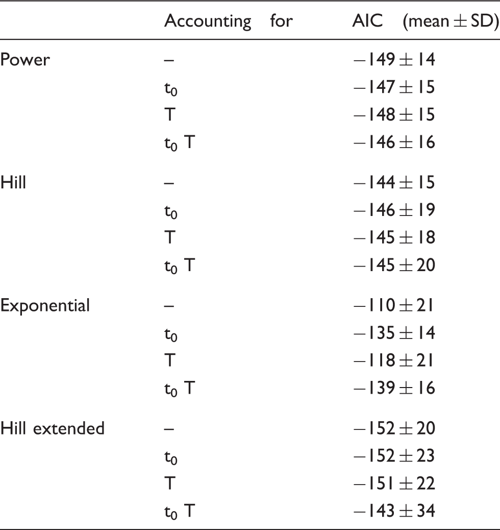
AIC scores for the model selection of [¹¹C]PBR28.

	Accounting for	AIC (mean ± SD)
Power	–	−149 ± 14
	t₀	−147 ± 15
	T	−148 ± 15
	t₀ T	−146 ± 16
Hill	–	−144 ± 15
	t₀	−146 ± 19
	T	−145 ± 18
	t₀ T	−145 ± 20
Exponential	–	−110 ± 21
	t₀	−135 ± 14
	T	−118 ± 21
	t₀ T	−139 ± 16
Hill extended	–	−152 ± 20
	t₀	−152 ± 23
	T	−151 ± 22
	t₀ T	−143 ± 34

Since the PPf value of the first sample (taken 15 seconds after injection) was smaller than 1 (0.95 ± 0.03) in each subject, all equations were implemented considering an initial PPf value ( ${PPf}_{0}$ ), estimated along with the other parameters, different from 1.

The estimation of the parameters was performed using a maximum-likelihood non-linear estimator with relative weights. These were defined as the inverse of the variance of each data point, and the variance was calculated using equation (8). A nonlinear constraint was imposed on the extended Hill model in order to ensure its positivity at late times.

Model selection

As a first step, we assessed whether the inclusion of the delay and the injection length significantly improved the fitting of the models, by comparing the AIC indices with paired t-tests.

Including the delay term significantly improved the fitting (i.e. lower AIC) of the exponential models (p = 0.002 against the standard exponential model and p = 0.007 for the version convoluted with injection length), but resulted in a significantly higher AIC for the power models (both standard and convoluted: p = 0.023 and p < 0.001, respectively). No significant differences were found for the Hill functions. Adding the injection length significantly reduced the AIC indices only for the exponential model (p = 0.013). Therefore, t₀ and T were added only to the exponential model.

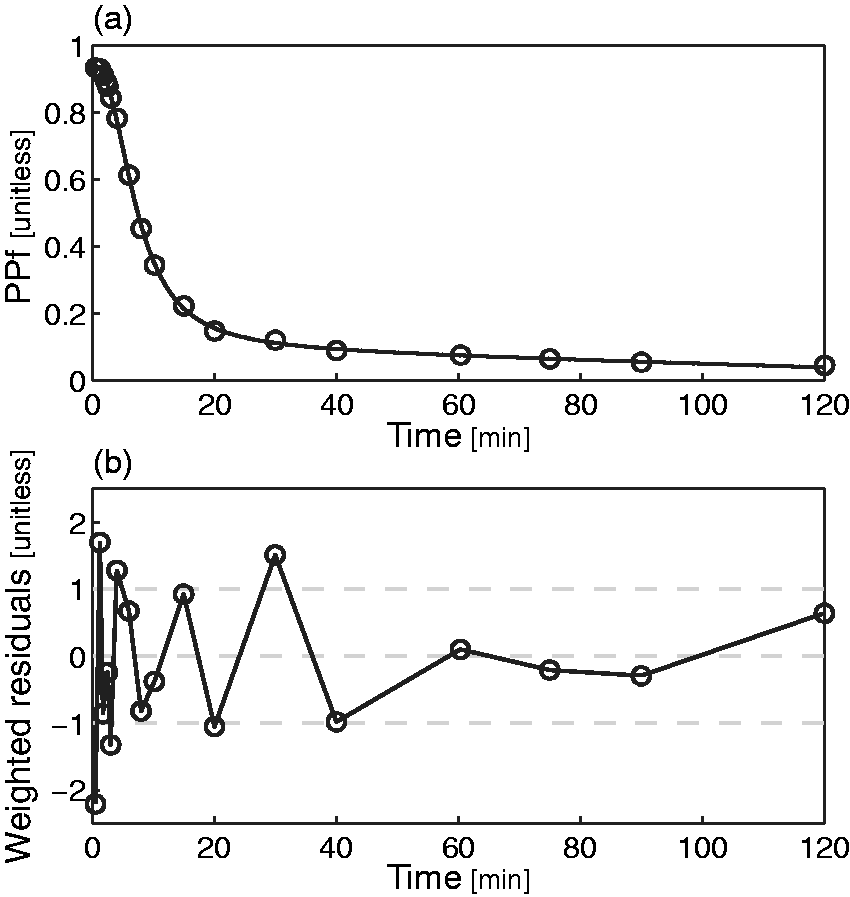
Among the four remaining models (exponential with t₀ and T, power, Hill and Hill extended), the extended Hill model had the lowest mean AIC (Table 2) albeit statistical significance (Bonferroni corrected) was reached only against the basic Hill model (p = 0.014). Notably, the exponential model showed unreliable estimates (CV > 100%) while the power model tended to overestimate the PPf curve around the 20th min (Figure 2a), thus producing a polarization of the weighted residuals. Therefore, both these models were rejected. The basic Hill model did not fit correctly the tails of the PPf curves (Figure 2b) because these did not reach a plateau level but decreased slowly and constantly. Among the tested alternatives, the extended Hill model showed the most reliable estimates (CV: a = 6 ± 9%, b = 0.04 ± 0.06%, c = 10 ± 19%, d = 6 ± 6%, PPf₀ = 1 ± 1%, ). The model adequately fitted the data and the weighted residuals were consistent with the measurement error hypotheses (both runs and Anderson-Darling tests did not detect assumptions violation) (Figure 2c). Therefore, the extended Hill model was selected to fit [¹¹C]PBR28 PPf curves. Figure 3 shows an example of fit and weighted residuals for a representative subject.

Figure 2.

Weighted residual comparison of the PPf models. Mean (black line) and between-subject variance (grey area) of the weighted residuals obtained by fitting the different PPf models to [¹¹C]PBR data: (a) power model with t₀ constrained to 0. (b) Hill model with t₀ constrained to 0. (c) Extended Hill model with t₀ fixed to 0. (D) Convoluted exponential model with estimated t₀. The Extended Hill model provided the best description of the data and was the only one to yield random residuals.

Figure 3.

Plasma parent fraction modeling with the extended Hill model. (a) Fitting of the [¹¹C]PBR28 PPf measurements (open circles) with the extended Hill model (black line) in a representative subject and (b) weighted residuals over time for the same subject.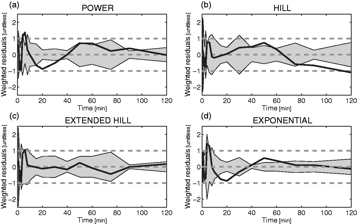

Tissue estimates were obtained as described in Rizzo et al.⁷⁵ using as PPf model the four alternatives selected in the first step. The impact on V_T varied according to the PPf model and ranged from $7 % \pm 5 %$ for the non-extended Hill model to $5 % \pm 10 %$ for the convoluted exponential model (versus the extended Hill model). The bias of the binding potential was higher and ranged from $- 5 % \pm 12 %$ to $- 25 % \pm 26 %$ .

Population approaches

In this section, we compared population-based curves to the individual fitting of the PPf performed with the optimal model selected in the previous section. In particular, we implemented the NLMEM approach as described in Veronese et al.⁵⁵ and the naïve average method by averaging the PPf samples of all subjects and then by fitting the average curve with the extended Hill model. For each subject, the PPf curve was thus estimated using the individual and the two population approaches and the estimation was repeated by progressively reducing the number of samples available (i.e. frequent, standard and sparse sampling). For each approach and each sampling frequency, we calculated the residual sum of squares (RSS) between the PPf curve estimated and all the available PPf datapoints, regardless of the samples used in the estimation. The individual fit obtained with frequent sampling was taken as reference. Notably, the number of samples obtained with sparse sampling was not sufficient to estimate the model parameters individually.

NLMEM could reliably recover the individual PPf with all sampling frequencies. The fit obtained with frequent sampling was not statistically different from that obtained with standard sampling (p < 0.05, paired t-test) and only borderline different (p = 0.046) from the fit obtained with sparse sampling (Figure 4).

Figure 4.

Comparison between individual, NLMEM and average fitting for the estimation of the PPf curve when the number of samples is reduced. Boxplots of the residual sum of squares (RSS) between the PPf curve estimated with the individual, NLMEM and average approach and all the PPf data available, regardless of the samples used in the estimation. Stars indicate statistical differences (p < 0.05) tested with pair t-tests. The robustness of the methods was tested by progressively reducing the number of data points: frequent sampling: with all the available PPf measurements of each subject (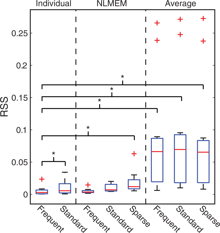 $19 \pm 1$ on average, for 120-min input functions); standard sampling: six samples per subject were used, as commonly found in the literature. The protocol used by Hannestad and colleagues⁷⁶ for [¹¹C]PBR28 was adopted (i.e. the samples were taken at 3, 8, 15, 30, 60, and 90 min after injection); sparse sampling: the number of PPf samples per subject was reduced to the minimal number necessary to fit the correspondent PPf model (i.e. 5, equal to the number of the parameters). In addition, for half of the population (six subjects randomly chosen, including the one presented in this figure) the number of samples was further reduced to 4. This was done in order to simulate the unexpected loss of a sample (e.g. arterial catheter failure, clotted blood, problems in HPLC analysis, etc.). Notably, the sparse sampling does not allow the estimation of the individual parameters of the model.

On the other hand, the model descriptions of the individual method were statistically different between standard and frequent sampling (which is expected, because the individual method does not use any additional information other than the data to analyze).

Finally, the PPf profile obtained from the average approach significantly differs from the profile measured individually (Figure 5). In general, the higher the population variability, the higher the error introduced by the average approach.

Figure 5.

Fit obtained with the individual, NLMEM and average approaches in a representative [¹¹C]PBR28 subject for different sampling frequencies. The PPf data points (open circles) of a representative [¹¹C]PBR28 subject were fitted using the individual model (black dashed line), NLMEM (black solid line) and the average approach (grey solid line) with frequent (a), standard (b), and sparse (c) samples.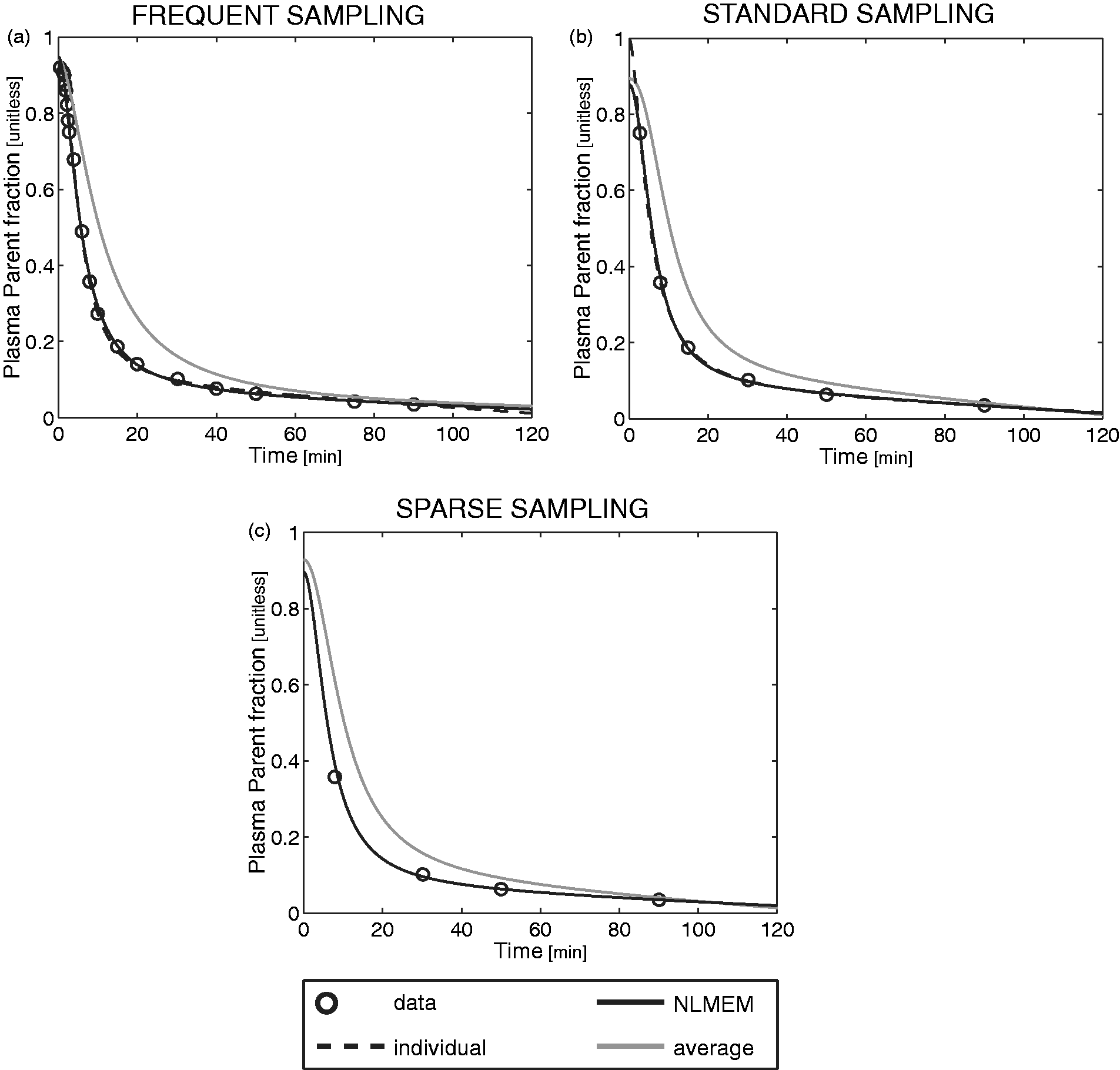

Conclusion

Correcting the input function for radiometabolites is a crucial step to obtain reliable estimates of tissue parameters. This is usually done by measuring the fraction of activity due to the parent tracer in plasma and then by fitting the data points with a mathematical model. In order to select the optimal plasma model among the many that are available in the literature, one should first preselect a suitable subset of PPf models, tailored to the characteristics of the radiotracer under analysis and to the experimental setting, and then carry out comprehensive comparisons.

In this review, we used a dataset of [¹¹C]PBR28 as case study to guide the reader through the process of model selection and we found that an extended Hill model provided the most accurate description of the PPf shape of this radioligand.

Finally, NLMEM can be used to obtain a robust radiometabolite correction when the number of samples available is too small for standard modeling approaches. Population approaches based on averaged PPf curves are not recommended because they can heavily bias arterial input shapes and therefore the tissue parameters.

Footnotes

Funding

The author(s) disclosed receipt of the following financial support for the research, authorship, and/or publication of this article: This work was supported in part by the Intramural Research Program, National Institute of Mental Health (ZIAMH002795) and by UK Medical Research Council programme (grant no. G1100809/1).

Acknowledgements

The authors are grateful to Dr Robert Innis for making the [¹¹C]PBR28 scans available for this review. Portions of this work were presented in preliminary form at Neuroreceptor Mapping (Amsterdam, 2014).

Declaration of conflicting interests

The author(s) declared no potential conflicts of interest with respect to the research, authorship, and/or publication of this article.

Authors’ contributions

MT, GR, MV, and AB contributed significantly to the overall work design. PZ-F, MF and SSZ provided the PET data that were then analysed by MT. SSZ contributed to radiochemistry data interpretation. MT prepared the manuscript with input from MV, GR, PZ-F, and AB.

References

Shields

Briston

Chandupatla

. A simplified analysis of [18F]3′-deoxy-3′-fluorothymidine metabolism and retention. Eur J Nucl Med Mol Imaging 2005; 32: 1269–1275.

Pike

. PET radiotracers: crossing the blood–brain barrier and surviving metabolism. Trends Pharmacol Sci 2009; 30: 431–440.

Kim

Szabo

Seki

. Effect of tracer metabolism on PET measurement of [11C]pyrilamine binding to histamine H1 receptors. Ann Nucl Med 1999; 13: 101–107.

Sasaki

Ito

Kimura

. Quantification of dopamine transporter in human brain using PET with 18F-FE-PE2I. J Nucl Med 2012; 53: 1065–1073.

Lubberink

Boellaard

Greuter

HNJM

. Effect of uncertainty in plasma metabolite levels on kinetic analysis of [11 C] flumazenil and [11 C] (R) -PK11195 PET studies. Neuroimage 2004; 22: T61–T200.

Parsey

Ojha

Ogden

. Metabolite considerations in the in vivo quantification of serotonin transporters using 11C-DASB and PET in humans. J Nucl Med 2006; 47: 1796–1802.

Ogden

Mann

. Optimal metabolite curve fitting for kinetic modeling of 11C-WAY-100635. J Nucl Med 2007; 48: 926–931.

Tonietto M, Veronese M, Rizzo G, et al. Improved models for plasma radiometabolite correction and their impact on kinetic quantification in PET studies. J Cereb Blood Flow 2015; 35: 1462–1469.

Watabe

Channing

Der

. Kinetic analysis of the 5-HT2A ligand [11C]MDL 100,907. J Cereb Blood Flow Metab 2000; 20: 899–909.

10.

Kimura

Ishii

Fukumitsu

. Quantitative analysis of adenosine A1 receptors in human brain using positron emission tomography and [1-methyl-11C]8-dicyclopropylmethyl-1-methyl-3-propylxanthine. Nucl Med Biol 2004; 31: 975–981.

11.

Meyer

Elmenhorst

Bier

. Quantification of cerebral A1 adenosine receptors in humans using [18F]CPFPX and PET: An equilibrium approach. Neuroimage 2005; 24: 1192–1204.

12.

Hinz

Bhagwagar

Cowen

. Validation of a tracer kinetic model for the quantification of 5-HT(2A) receptors in human brain with [(11)C]MDL 100,907. J Cereb Blood Flow Metab 2007; 27: 161–172.

13.

Gunn

Sargent

Bench

. Tracer kinetic modeling of the 5-HT1A receptor ligand [carbonyl-11C]WAY-100635 for PET. Neuroimage 1998; 8: 426–440.

14.

Lubberink

Luurtsema

van Berckel

BNM

. Evaluation of tracer kinetic models for quantification of P-glycoprotein function using (R)-[11C]verapamil and PET. J Cereb Blood Flow Metab 2007; 27: 424–433.

15.

Hirvonen

Johansson

Teräs

. Measurement of striatal and extrastriatal dopamine transporter binding with high-resolution PET and [11C]PE2I: Quantitative modeling and test-retest reproducibility. J Cereb Blood Flow Metab 2008; 28: 1059–1069.

16.

Klumpers

UMH

Veltman

Boellaard

. Comparison of plasma input and reference tissue models for analysing [(11)C]flumazenil studies. J Cereb Blood Flow Metab 2008; 28: 579–587.

17.

Yaqub

Boellaard

van Berckel

BNM

. Evaluation of tracer kinetic models for analysis of [18 F]FDDNP studies. Mol Imaging Biol 2009; 11: 322–333.

18.

Endres

Pomper

James

. Initial evaluation of 11C-DPA-713, a novel TSPO PET ligand, in humans. J Nucl Med 2009; 50: 1276–1282.

19.

Jučaite

Cselényi

Arvidsson

. Kinetic analysis and test-retest variability of the radioligand [11C](R)-PK11195 binding to TSPO in the human brain – a PET study in control subjects. EJNMMI Res 2012; 2: 15.

20.

Roivainen

Någren

Hirvonen

. Whole-body distribution and metabolism of [N-methyl-11C](R)-1-(2-chlorophenyl)-N-(1-methylpropyl)-3-isoquinolinecarboxamide in humans; an imaging agent for in vivo assessment of peripheral benzodiazepine receptor activity with positron emission tomography. Eur J Nucl Med Mol Imaging 2009; 36: 671–682.

21.

Tsujikawa

Zoghbi

Hong

. In vitro and in vivo evaluation of 11C-SD5024, a novel PET radioligand for human brain imaging of cannabinoid CB1 receptors. Neuroimage 2014; 84: 733–741.

22.

Luoto P, Suilamo S, Oikonen V, et al. 11C-ORM-13070, a novel PET ligand for brain α2C-adrenoceptors: radiometabolism, plasma pharmacokinetics, whole-body distribution and radiation dosimetry in healthy men. Eur J Nucl Med and Mol Imag 2014; 41: 1947–1956.

23.

Guo

Colasanti

Owen

. Quantification of the specific translocator protein signal of 18F-PBR111 in healthy humans: a genetic polymorphism effect on in vivo binding. J Nucl Med 2013; 54: 1915–1923.

24.

Owen

Guo

Kalk

. Determination of [11C]PBR28 binding potential in vivo: A first human TSPO blocking study. J Cereb Blood Flow Metab 2014; 34: 989–994.

25.

Endres

Bencherif

Hilton

. Quantification of brain μ-opioid receptors with [11C]carfentanil: Reference-tissue methods. Nucl Med Biol 2003; 30: 177–186.

26.

Asselin

M-C

Montgomery

Grasby

. Quantification of PET studies with the very high-affinity dopamine D2/D3 receptor ligand [11C]FLB 457: re-evaluation of the validity of using a cerebellar reference region. J Cereb Blood Flow Metab 2007; 27: 378–392.

27.

Edison

Brooks

Turkheimer

. Strategies for the generation of parametric images of [11C]PIB with plasma input functions considering discriminations and reproducibility. Neuroimage 2009; 48: 329–338.

28.

Contractor

Kenny

Coombes

. Evaluation of limited blood sampling population input approaches for kinetic quantification of [18F]fluorothymidine PET data. EJNMMI Res 2012; 2: 11.

29.

Tarkia

Saraste

Saanijoki

. Evaluation of 68Ga-labeled tracers for PET imaging of myocardial perfusion in pigs. Nucl Med Biol 2012; 39: 715–723.

30.

Hawkins

Huang

Barrio

. Estimation of local cerebral protein synthesis rates with L-[1-11C]leucine and PET: methods, model, and results in animals and humans. J Cereb Blood Flow Metab 1989; 9: 446–460.

31.

Magata

Mukai

Ihara

. Simple analytic method of 11C-flumazenil metabolite in blood. J Nucl Med 2003; 44: 417–421.

32.

Ishiwata

Itou

Ohyama

. Metabolite analysis of [11C]flumazenil in human plasma: assessment as the standardized value for quantitative PET studies. Ann Nucl Med 1998; 12: 55–59.

33.

Abi-Dargham

Simpson

Kegeles

. PET studies of binding competition between endogenous dopamine and the D1 radiotracer [11C]NNC 756. Synapse 1999; 32: 93–109.

34.

Ikoma

Yasuno

Ito

. Quantitative analysis for estimating binding potential of the peripheral benzodiazepine receptor with [(11)C]DAA1106. J Cereb Blood Flow Metab 2007; 27: 173–184.

35.

Park-Holohan S-J, Asselin M-C, Turton DR, et al. Quantification of [11C]GB67 binding to cardiac α1-adrenoceptors with positron emission tomography: validation in pigs. Eur J Nucl Med Mol Imaging 2008; 35(9): 1624–1635.

36.

Peyronneau

Saba

Goutal

. Metabolism and quantification of [18F]DPA-714, a new TSPO positron emission tomography radioligand. Drug Metab Dispos 2013; 41: 122–131.

37.

Kropholler

Boellaard

Schuitemaker

. Development of a tracer kinetic plasma input model for (R)-[11C]PK11195 brain studies. J Cereb Blood Flow Metab 2005; 25: 842–851.

38.

Lammertsma

Bench

Price

. Measurement of cerebral monoamine oxidase B activity using L-[11C]deprenyl and dynamic positron emission tomography. J Cereb Blood Flow Metab 1991; 11: 545–556.

39.

Buck a, Wolpers

Hutchins

. Effect of carbon-11-acetate recirculation on estimates of myocardial oxygen consumption by PET. J Nucl Med 1991; 32: 1950–1957.

40.

Wyss

Weber

Treyer

. Stimulation-induced increases of astrocytic oxidative metabolism in rats and humans investigated with 1-11C-acetate. J Cereb Blood Flow Metab 2009; 29: 44–56.

41.

Hammers

Asselin

Turkheimer

. Balancing bias, reliability, noise properties and the need for parametric maps in quantitative ligand PET: [11C]diprenorphine test-retest data. Neuroimage 2007; 38: 82–94.

42.

Searle

Beaver

Tziortzi

. Mathematical modelling of [¹¹C]-(+)-PHNO human competition studies. Neuroimage 2013; 68: 119–132.

43.

Lamare

Hinz

Gaemperli

. Detection and quantification of large-vessel inflammation with 11C-(R)-PK11195 PET/CT. J Nucl Med 2011; 52: 33–39.

44.

Carson

Breier

de Bartolomeis

. Quantification of amphetamine-induced changes in [11C]raclopride binding with continuous infusion. J Cereb Blood Flow Metab 1997; 17: 437–447.

45.

Naganawa

Jacobsen

Zheng

. Evaluation of the agonist PET radioligand [11C]GR103545 to image kappa opioid receptor in humans: Kinetic model selection, test-retest reproducibility and receptor occupancy by the antagonist PF-04455242. Neuroimage 2014; 99: 69–79.

46.

Lohith

Zoghbi

Morse

. Brain and whole-body imaging of nociceptin/orphanin FQ peptide receptor in humans using the PET ligand 11C-NOP-1A. J Nucl Med 2012; 53: 385–392.

47.

Oikonen V. Effect of tracer metabolism during sample preparation. In: XIII Turku PET symposium 24–27 May 2014, Turku, Finland.

48.

Lohith

Tsujikawa

. Evaluation in monkey of two candidate PET radioligands, [11C]RX-1 and [18F]RX-2, for imaging brain 5-HT 4 receptors. Synapse 2014; 68: 613–623.

49.

Cobelli C, Foster D and Toffolo G. 2000. Tracer Kinetics in Biomedical Research. New York: Springer.

50.

Carson E, Cobelli C, Karbing DS, et al. Modelling Methodology for Physiology and Medicine. 2nd edn, London: Elsevier Inc., 2014.

51.

Akaike H. A new look at the statistical model identification. IEEE Transactions on Automatic Control 1974; 19(6): 716–723.

52.

Schwarz

. Estimating the dimension of a model. Ann Stat 1978; 6: 461–464.

53.

Stephan

Penny

Daunizeau

. Bayesian model selection for group studies. Neuroimage 2009; 46: 1004–1017.

54.

Veronese

Gunn

Zamuner

. A non-linear mixed effect modelling approach for metabolite correction of the arterial input function in PET studies. Neuroimage 2013; 66: 611–622.

55.

Lammertsma

Bench

Hume

. Comparison of methods for analysis of clinical [11C]raclopride studies. J Cereb Blood Flow Metab 1996; 16: 42–52.

56.

Okazawa

Yamauchi

Sugimoto

. Effects of metabolite correction for arterial input function on quantitative receptor images with 11C-flumazenil in clinical positron emission tomography studies. J Comput Assist Tomogr 2004; 28: 428–435.

57.

Mitkovski

Villemagne

Novakovic

. Simplified quantification of nicotinic receptors with 2[18F]F-A-85380 PET. Nucl Med Biol 2005; 32: 585–591.

58.

Backes

Ullrich

Neumaier

. Noninvasive quantification of 18F-FLT human brain PET for the assessment of tumour proliferation in patients with high-grade glioma. Eur J Nucl Med Mol Imaging 2009; 36: 1960–1967.

59.

Zanotti-Fregonara

Chen

Liow

J-S

. Image-derived input function for brain PET studies: many challenges and few opportunities. J Cereb Blood Flow Metab 2011; 31: 1986–1998.

60.

Henriksen

Spilker

Sprenger

. Gender dependent rate of metabolism of the opioid receptor–PET ligand F-18-fluoroethyl-diprenorphine. J Cereb Blood Flow Metab 2005; 25: S628–S628.

61.

Visvikis

Francis

Mulligan

. Comparison of methodologies for the in vivo assessment of 18FLT utilisation in colorectal cancer. Eur J Nucl Med Mol Imag 2004; 31: 169–178.

62.

Davidian

Giltinan

. Nonlinear models for repeated measurement data: An overview and update. J Agric Biol Environ Stat 2003; 8: 387–419.

63.

Huang

Barrio

. Modelling approach for separating blood time-activity curves in positron emission tomographic studies. Phys Med Biol 1991; 36: 749–761.

64.

Gunn

Cunningham

. Positron emission tomography compartmental models. J Cereb Blood Flow Metab 2001; 21: 635–652.

65.

Cumming

Léger

Kuwabara

. Pharmacokinetics of Plasma 6-[18F]Fluoro-L-3,4-dihydroxyphenylalanine[18F]FDOPA in Humans. J Cereb Blood Flow Metab 1993; 13: 668–675.

66.

Kuwabara

Cumming

Reith

. Human striatal L-dopa decarboxylase activity estimated in vivo using 6-[18F]fluoro-dopa and positron emission tomography: error analysis and application to normal subjects. J Cereb Blood Flow Metab 1993; 13: 43–56.

67.

Mankoff

Shields

Graham

. Kinetic analysis of 2-[carbon-11]thymidine PET imaging studies: compartmental model and mathematical analysis. J Nucl Med 1998; 39: 1043–1055.

68.

Burger

Buck

. Tracer kinetic modelling of receptor data with mathematical metabolite correction. Eur J Nucl Med 1996; 23: 539–545.

69.

Sanabria-Bohórquez

Labar

Levêque

. [11C]Flumazenil metabolite measurement in plasma is not necessary for accurate brain benzodiazepine receptor quantification. Eur J Nucl Med 2000; 27: 1674–1683.

70.

Chiou

. The phenomenon and rationale of marked dependence of drug concentration on blood sampling site. Implications in pharmacokinetics, pharmacodynamics, toxicology and therapeutics (Part I). Clin Pharmacokinet 1989; 17: 175–199.

71.

Chiou

72.

Zanotti-Fregonara

Leroy

Rizzo

. Imaging of monoamine oxidase-A in the human brain with [11C]befloxatone: quantification strategies and correlation with mRNA transcription maps. Nucl Med Commun 2014; 35: 1254–1261.

73.

Hines

Fujita

Zoghbi

. Propofol decreases in vivo binding of 11C-PBR28 to translocator protein (18 kDa) in the human brain. J Nucl Med 2012; 54: 64–69.

74.

Zoghbi

Shetty

Ichise

. PET imaging of the dopamine transporter with 18F-FECNT: A polar radiometabolite confounds brain radioligand measurements. J Nucl Med 2006; 47: 520–527.

75.

Rizzo

Veronese

Tonietto

. Kinetic modeling without accounting for the vascular component impairs the quantification of [(11)C]PBR28 brain PET data. J Cereb Blood Flow Metab 2014; 34: 1060–1069.

76.

Hannestad

DellaGioia

Gallezot

. The neuroinflammation marker translocator protein is not elevated in individuals with mild-to-moderate depression: A [11C]PBR28 PET study. Brain Behav Immun 2013; 33: 131–138.

Plasma radiometabolite correction in dynamic PET studies: Insights on the available modeling approaches

Abstract

Keywords

Introduction

Plasma parent fraction modeling

Power models

Hill models

Exponential models

Modeling the appearance of radiometabolites and the parameters of injection

Accounting for measurement errors

Model selection

Population approaches

Unconventional approaches

Compartmental models

Radiometabolite correction without metabolite measurements

Radiometabolite correction with venous sampling

Case study: [11C]PBR28

Dataset

PPf modeling

Model selection

Population approaches

Conclusion

Footnotes

Funding

Acknowledgements

Declaration of conflicting interests

Authors’ contributions

References

Case study: [¹¹C]PBR28