
Abstract
It is important to be able to predict the life of materials at high temperatures. The Monkman-Grant relation offers potential for reducing the development cycle for new materials. This paper uses the 4-θ methodology to i. identify and explain the form of this relation in terms of creep mechanisms and ii. to discover whether this form is compatible with development cycle reduction. The Monkman-Grant proportionality constant (M2) was found to fall into three groupings depending on the amount of damage and the rate at which this occurred. Only once this was considered did the exponent on the secondary creep rate equal −1 – as predicted by 4-θ methodology. One of these groupings might be relevant for longer term life assessment.
Introduction
12Cr-1Mo-V-Nb steel (also referred to as T12 steel or ASTM A387 Grade 12: Class 2 steel) is a type of low-alloy steel that is often classified as a heat-resistant steel. The alloying elements contained within it contribute to its enhanced strength and creep resistance at high temperatures, as well as its good resistance to oxidation and good weldability properties. It is currently used in ultra-super-critical boilers as superheater and reheater tubes that typically operate at temperatures at or above 873 K and stresses exceeding 25 MPa. It is also a material considered for use in advanced nuclear reactors – including fourth generation nuclear reactors. These reactors typically operate in the range 1025 K to 1273 K and a range of 5 to 10 MPa. While it is not commonly used for critical turbine components like blades or rotors, this steel can be used for the parts of turbines that are exposed to less extreme temperatures and stresses where good resistance to creep and oxidation is required.
For the safe and economic operation of such components and systems, a creep rupture life in the time range of 105 h is required. Evaluation of such long-term creep rupture is typically done using accelerated creep tests (either accelerated stresses and or temperatures), with creep models then being used to extrapolate to the lower stresses observed in the above-mentioned systems. However, there is little agreement on what creep models extrapolate best with respect to stress and temperature, and whilst some more recently developed models have been shown to perform well at such extrapolation over a wide range of materials, they currently lack the theoretical backing that provides the additional confidence required for widespread adoption (for example, Yang et al. 1 and Wilshire et al.2–6). An analysis of minimum creep rates vs. times to failure – the so called Monkman–Grant relation 7 – using accelerated test data is another suggested way to evaluate long-term creep rupture by extrapolating this accelerated relation via smaller minimum creep rates – because once the minimum rate of creep in an on-going creep test at non accelerated stresses is obtained at an early stage of creep, its rupture life is readily evaluated from this accelerated relation without a need to extrapolate with respect to stress and/or temperature.
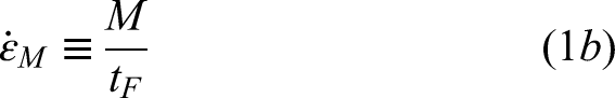
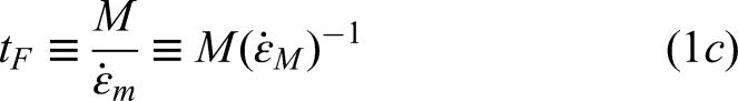
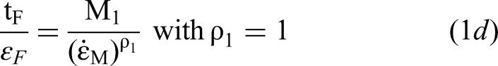
A relationship between time to failure tF and the minimum creep rate
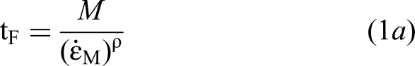
At a specific test condition, and when ρ = 1, the Monkman-Grant equation is a simple tautology or identity (represented by the symbol
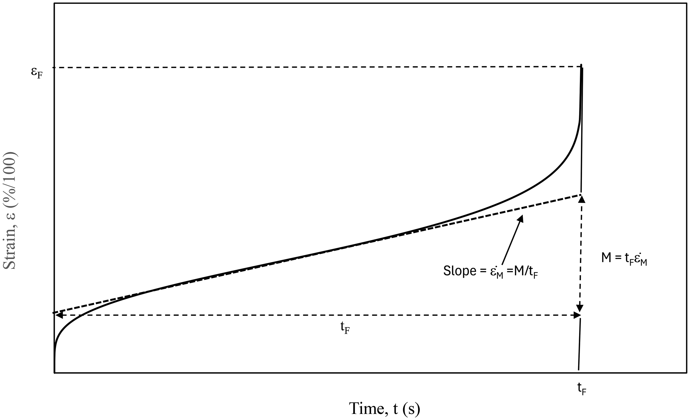
Schematic representation of a uniaxial creep curve obtained at a constant stress and temperature.
From this perspective, the Monkman-Grant relation requires the additional assumption that M is the same at all stresses and temperatures (subject to stochastic or random experimental variation). This assumption then turns this simple identity into a useful model or casual relation, because it then follows that a fall in
Since this relation was first identified, some doubt has been cast as to the constancy of M and ρ with respect to test conditions. For example, when studying 9Cr-1Mo steel, Abe
9
and Choudary
10
have shown M and ρ are different in value at long failure times (i.e., at lower stresses) compared to short and intermediate failure times. More specifically, these authors found that over most test conditions ρ = 1, but at the lower stresses leading to the longest failure times, ρ fell below 1. In order explain the change in values for M and ρ at lower stresses, several modifications of Equation (1a) have been proposed. Dobes and Milicka
11
proposed the following modified form
Abe
9
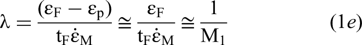
attributed the deviation from the simple MG relation with ρ = 1 in long-term creep, to increases in dln(ε˙)/dε, and proposed the following MG relation
Maruyama et al. 13 have also studied the phenomenon of ρ < 1 using data on 9Cr-1Mo (Grade 92) steel. They found that the value for ρ differed over four different regions of stress and temperature, where each of these regions corresponded to different creep mechanisms. Whilst the value for ρ over all tests was 0.85, they found it to be especially low (0.62) in a region corresponding to values of stress and temperature that induced long times to failure (in excess of 104 h). With long-term data points deviating from a MG relation determined from short-term data points, it becomes impossible to then use this relationship to evaluate long term life from short term data.
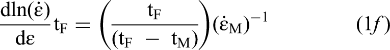
These authors then went onto to study the role played by creep curve shape in determining the values for M and ρ using the following equation

However, Equation (2a) is purely empirical in nature and its parameters have not been explained in terms of creep mechanisms. The aim of this paper is to identify a modified Monkman-Grant relation whose parameters can be explained in terms of creep processes such as hardening, softening and damage mechanisms. To do this, a similar material to that studied by Maruyama et al.
13
was selected – namely a Grade 12 steel – but the creep equation used was that from the 4-θ methodology developed by Evans and Wilshire
14

The use of the 4-θ methodology enables deviations from the Monkman-Grant relation of Equations (1b, 1c) to be explained not just in terms of creep curve shape, but also mechanisms governing creep. More specifically, this paper will derive a MG relation from the 4-θ methodology to gain insights into the roles played by creep hardening, softening and damage mechanisms in determining the form of the MG relation – and indeed whether these mechanisms change with test conditions. This will then enable insights to be made as to whether and how the MG relation in short term data can be used to evaluate long term rupture. To achieve these aims, the paper is structured as follows. The next section describes the creep tests carried out on Grade 12 steel, and this is followed by a method section outlining how a MG relation can be derived from the 4-θ methodology. This modified relation is then applied to data on 12Cr steel in the results section. Finally, the conclusion section outlines areas for future work.
The data
This section describes the data (which has not been previously published) used in this paper in more detail. Thirty-six cylindrical test pieces were machined from an as received batch of 12Cr-Mo-V-Nb steel. The chemical composition of this batch of material is shown in Table 1. The material was heat treated at 1423 K followed by air cooling and then two rounds of 3 h at 923 K (followed by air cooling each time). The tensile strength (σTS) for this batch of material is 990 MPa at room temperature and 551 MPa at 873 K, with corresponding 0.2% proof stresses of 831 MPa and 440 MPa. The specimens were tested in tension over a range of stresses and temperatures using high precision in Andrade-Chalmers constant-stress machines at the Interdisciplinary Research Centre (IRC) laboratories at Swansea University. Loads and stresses were applied and maintained to an accuracy of 0.5%. In all cases, temperatures were controlled along the gauge lengths and with respect to time to better than ±1 K. The extensometer could measure tensile strain to better than 10−5. Loading machines, extensometers and thermocouples were all calibrated with respect to NPL traceable standards.
Chemical composition (weight %).
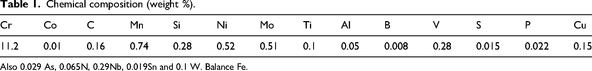
Also 0.029 As, 0.065N, 0.29Nb, 0.019Sn and 0.1 W. Balance Fe.
The test matrix used for this paper is shown in Table 2, where it can be noted that at three different test conditions a replicate test was carried out. Up to 403 creep strain/time readings were taken during each of these tests and Figure 2 shows the normalised experimental creep curves obtained at 873 K and various stresses. At these test conditions there are well defined primary and tertiary components to creep and a long period where the creep rate is constant – sometimes referred to as the secondary creep.
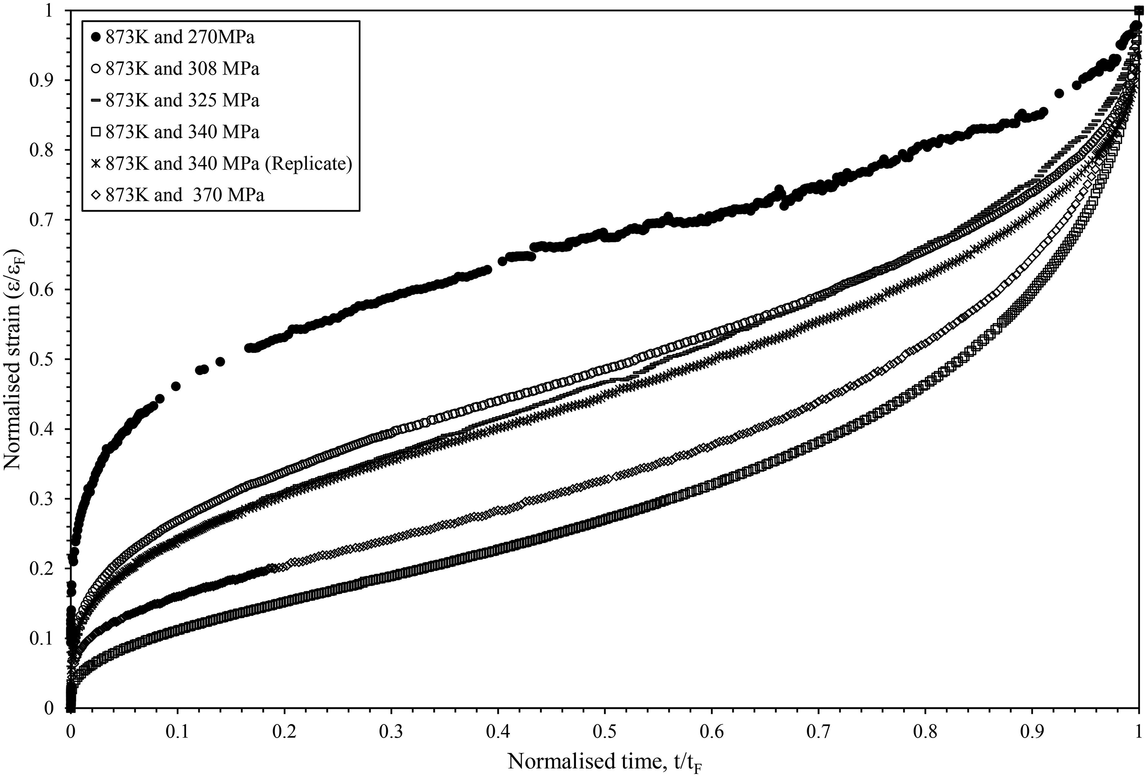
Normalised creep curves obtained from uniaxial tests carried out at 873 K and various stresses.
Test conditions for each of the 36 cut specimens.
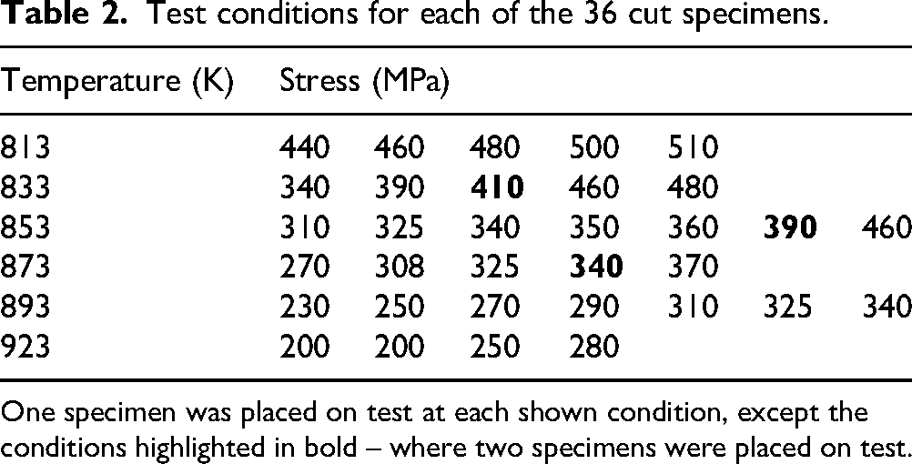
One specimen was placed on test at each shown condition, except the conditions highlighted in bold – where two specimens were placed on test.
Methodology
Creep mechanisms behind the 4-θ methodology
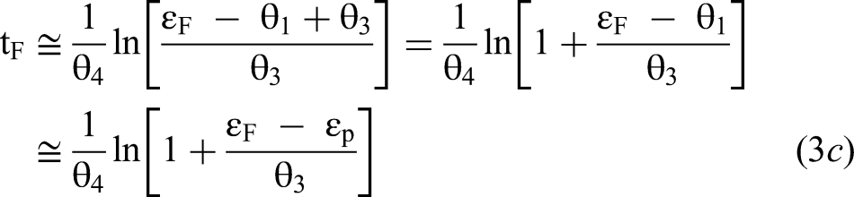
Based on Equation (2c), a specimen on test under uniaxial constant stress and temperature will eventually rupture with a failure time tF and with a strain at rupture of εF
Given that -θ2 is a small negative number and tF a large number, 


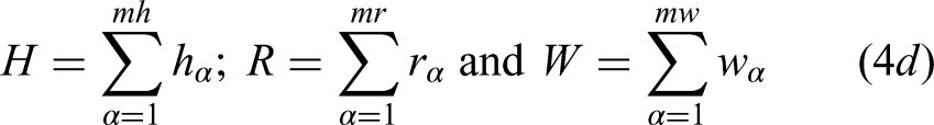
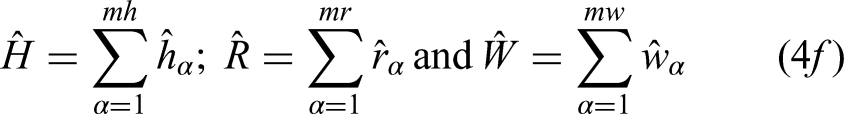
Evans then postulated the following evolutionary equations for all the internal variables

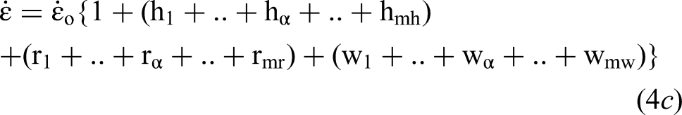
Equation (4c) can then be written as
Hardening refers to any phenomenon that leads to a slowing down of the creep rate, whilst softening leads to accelerating creep rates. Equation (4g) evaluates creep rates at any point in time relative to the creep rate measured at the start of the test
These characteristics have also been observed by Kafexhiu et al.
16
for this material. For example, these authors noted that at 873 K and 150 MPa, primary creep lasts only a few hours, followed by a prolonged secondary stage. Their long-term data (e.g., 10,000+ hours) showed secondary and tertiary creep domination. Consequently, the value of W in Equation (4g) remains close to zero for a large proportion of the overall creep time, so that the primary and secondary creep strain rate can be modelled as

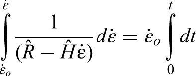
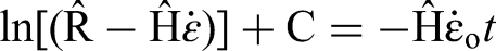
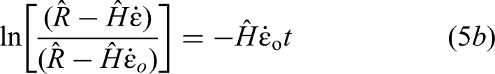
Next exponentiate both sides and then multiple both sides by 
Then solving for 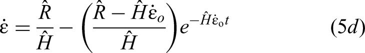
Then distribute and rearrange to yield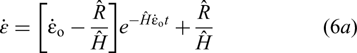
Equation (6a) states that an initial high creep rate of 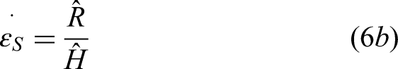
The value for this secondary creep rate is determined by the rate of work hardening 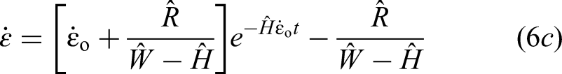
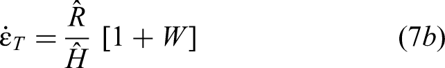
Now the secondary creep rate is determined by the rate of recovery relative to the excess of the hardening rate over the damage rate
The Monkman-Grant relation and damage
A second key assumption behind Equation (2c), that is also key to a more in depth understanding of the Monkman-Grant relation, is that damage W leads to strain rate accumulation by accelerating the secondary creep rate 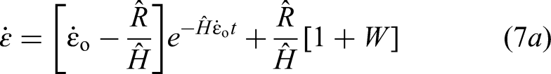
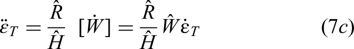
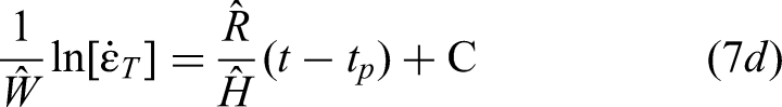
The next step is to perform an integration over the times and strains associated with tertiary creep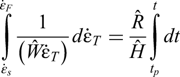
When t = tp the initial tertiary creep rate will equal the steady state creep rate, i.e., 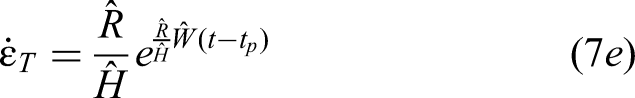
But for this material, Figure 2 reveals that tp is very small relative to tF so that 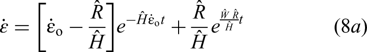
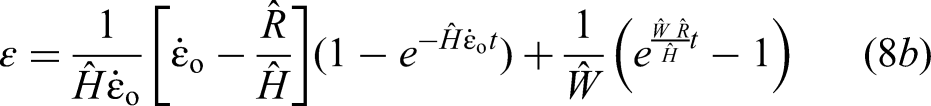
An important advantage of this theta methodology is that all the internal variables can be easily and directly calculated from the θ values describing a uniaxial creep curve. So, comparing Equations (8b) to (2c), it follows that
This approach makes it particularly useful for finite element modelling of more complex structures and situations where the stress is continually changing during the deformation process – e.g., in modelling the small punch test. Instead of using strain, time or life fraction hardening rules in such models, the estimated theta parameters can be used to recompute H, R and W, when there are changes in stress – which in combination with Equation (4g) allows the new point on the new stress creep rate curve to be quantified.
Equation (8c) is another way of showing that the two assumptions or approximations made in the derivation of Equations (8a, 8b) do not remove the appearance of damage from primary creep. In Equation (8c) θ3 determines the rate of damage accumulation
From Equation (8c) 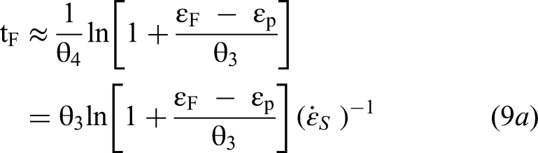
This is a Monkman-Grant type relation with 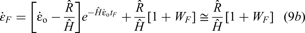
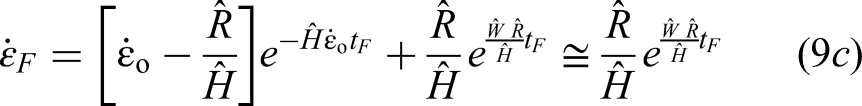
From Equations (9b, 9c)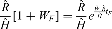

As an approximation

Substituting Equations (9d) into (9e)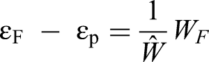

Evans 15 made it clear that WF does not have any units and it therefore dimensionless. Thus, what is consider a high value for WF is material specific. At first sight this raises concerns about physical interpretation, but past studies on other materials such as Waspaloy17,18 and have shown that WF depends directly on stress and indirectly on temperature via the material's tensile strength. Such a functional relationship can then be used to calculate the damage level that will induce failure at any test condition, and thus when failure will occur.
This then allows Equation (9a) to be written as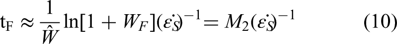
The role of primary creep in the determination of time to failure is limited to
In summary, the 4-θ methodology suggests M2 will be larger the more the material can tolerate significant creep strain or stress relaxation before damage (e.g., voids, microcracks) leads to failure. It also suggests that M2 will be larger the slower this damage accumulates over time. So, whether
Measuring minimum creep rates
The actual or observed creep rate at a given test condition is measured from the experimental creep curve. If such a curve is made up of i = 1 to n strain-time pairings, then the first step is to create a smoothed series for the experimental rates of strain using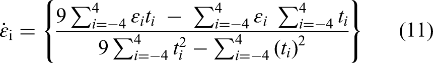
Figure 3 shows this smoothed experimental strain rate obtained at 440 MPa and 813 K. The observed minimum creep rate is not taken to be the smallest observed value, but the mean of the strain rates along the flat part of the strain rate curve. This observed minimum strain rate is what is usually shown in papers when studying the Monkman-Grant relation and is therefore represented by the symbol
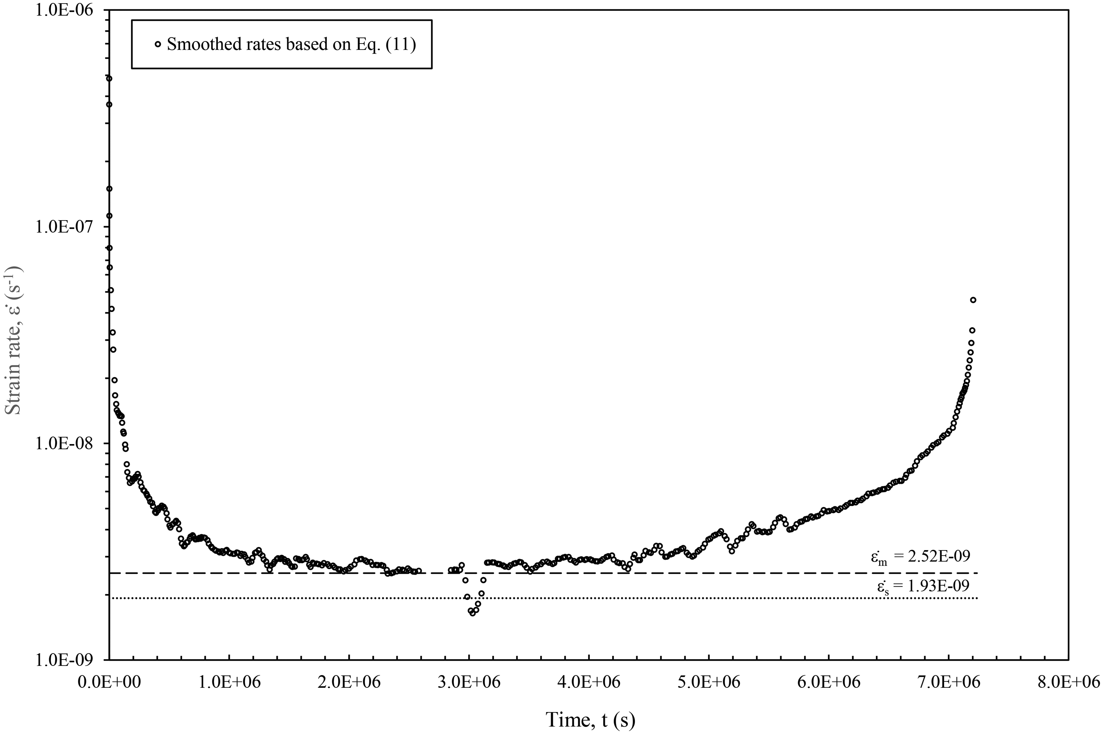
Smoothed experimental strain rates at 440 MPa and 813 K obtained using Equation (11), together with an estimate for the minimum creep rate and theoretical secondary rate.
In contrast to this, the theoretical secondary rate 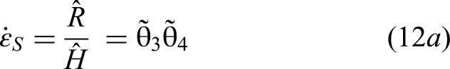
The rate of damage accumulation can be measured as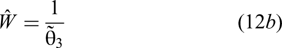
All the other internal rates can also be measured from the parameters of the fitted creep curve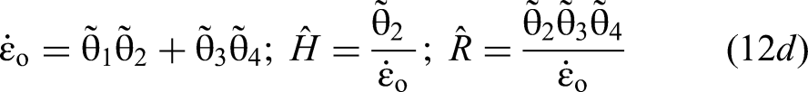
At 440 MPa and 813 K the estimates for θ3 and θ4 are
Results
Estimated values for each theta parameter and rates of hardening, softening and damage
Table 3 summarises the estimated values for each theta parameter at each test condition. These values are then inserted into Equations (12b, 12c, 12d) to obtain values for the rates of hardening, softening and damage. Such values are visualised in Figures 4–6.
Variation of a. the estimates made for the hardening proportionality constant
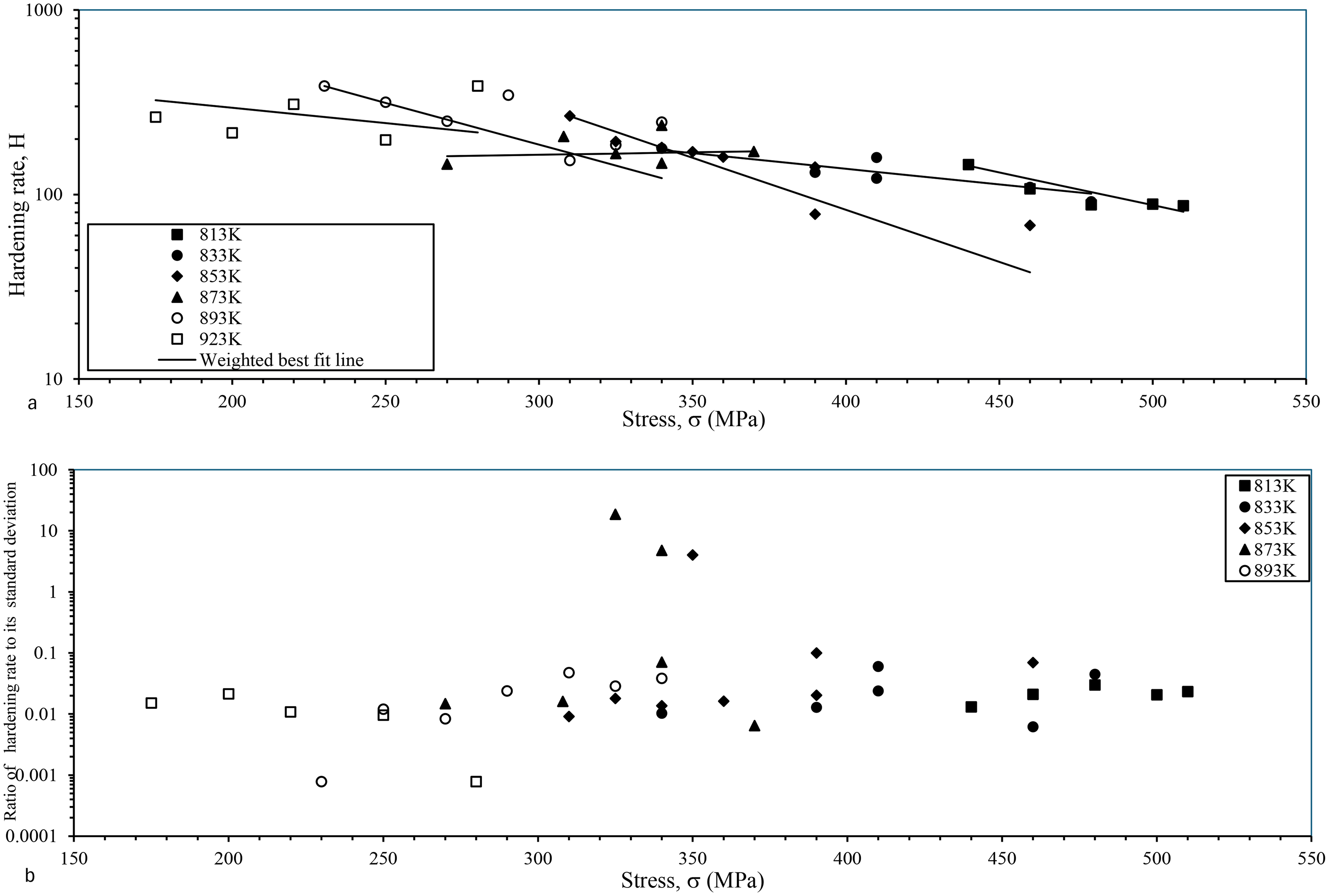
Variation of a. the estimates made for the softening proportionality constant
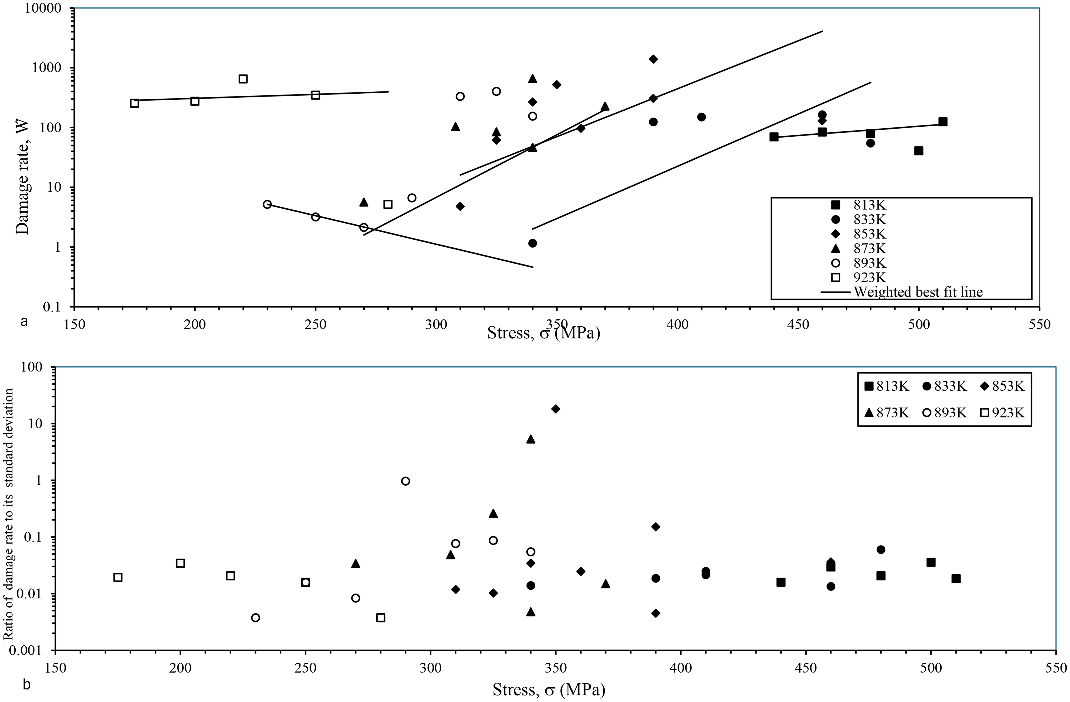
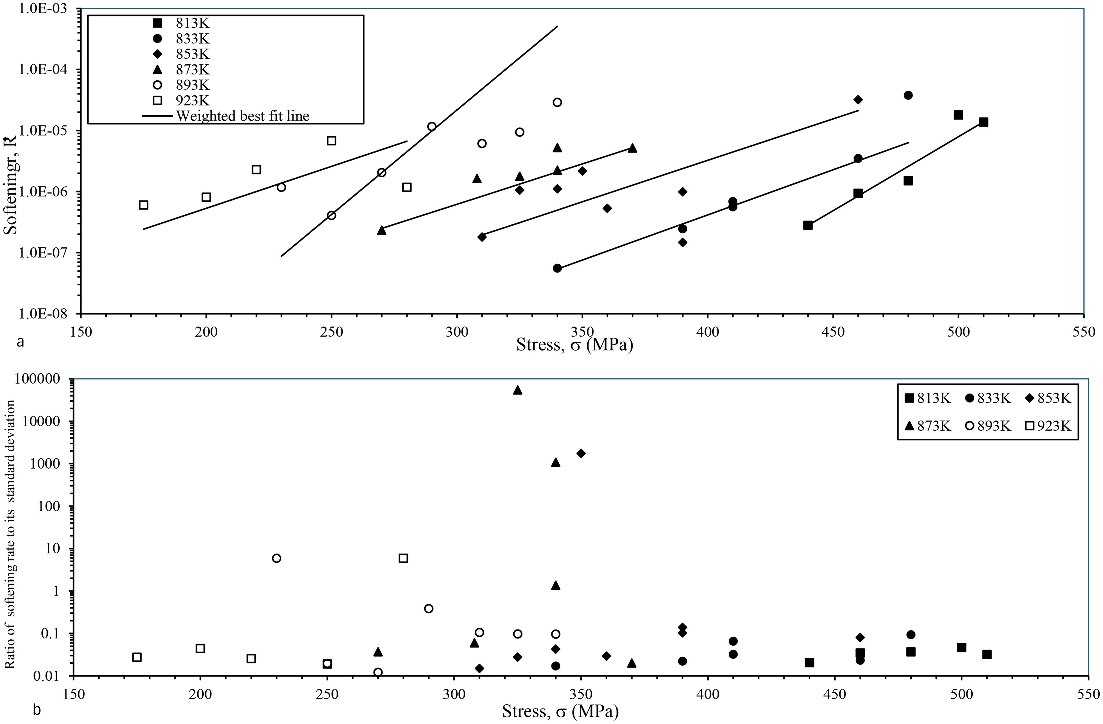
Variation of a. the estimates made for the damage proportionality constant
Estimated theta values by test condition.
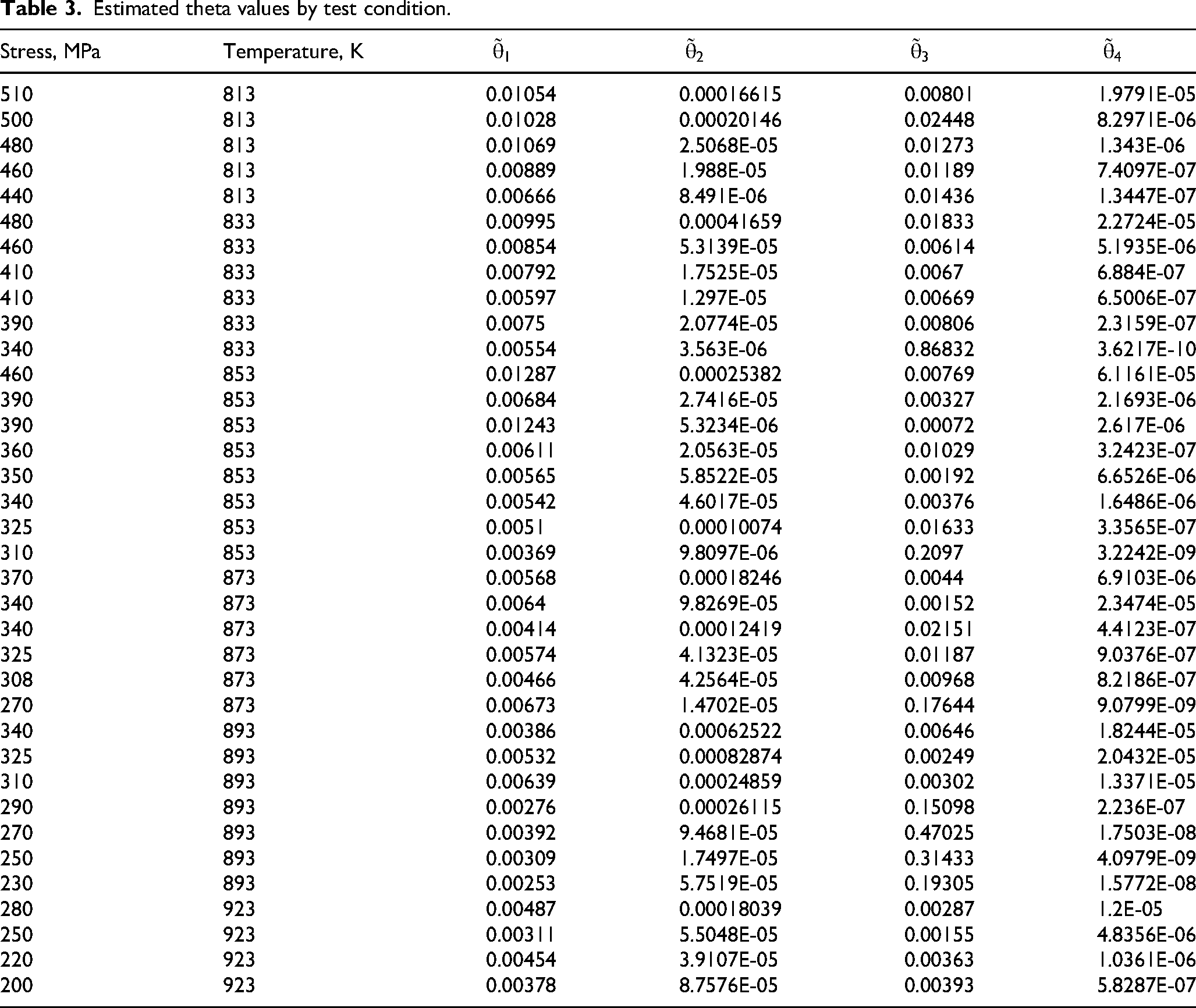
Figure 4(a) shows the estimates made for the proportionality constant determining the hardening rate at each test condition, together with the weighted isothermal best fit lines. The weights used are the inverses of the values given in Figure 4(b) where the ratio of each hardening constant to its standard deviation are plotted. Irrespective of temperature, decreasing stress tends to lead to an increase in the hardening constant, as so other things being equal, to a lower minimum creep rate and a smaller reduction in the creep rate as time progresses during tertiary creep. Typically, the standard deviation associated with each hardening constant is around 1% of the estimated value, but at 873 K, two of the hardening constant estimates are very unreliable and at 853 K one hardening constant estimate is unreliable as revealed by very high ratios in Figure 4(b). These three data points therefore play a small role in the determination of the shape of the weighted best fit lines.
Figure 4(a) reveals that the hardening constant declines with increases in both stress and temperature. Han et. al. 20 found that in 12Cr-1Mo-V-Nb steels, increased stress and temperature accelerate the coarsening of MX precipitates, leading to a decrease in the material's resistance to creep deformation. This coarsening reduces the effectiveness of precipitate strengthening, resulting in lower creep hardening rates. Higher stresses and temperatures can lead to the annihilation of dislocations, reducing the dislocation density. Since dislocations contribute to work hardening, their reduction leads to a decrease in the material's ability to harden during creep deformation.
Figure 5(a) shows the estimates made for the proportionality constant determining the softening rate at each test condition, together with the weighted iso-thermal best fit lines. Figure 5(b) plots the ratio of each softening rate to its standard deviation. Unlike for the hardening, the effect of an increase in stress at a given temperature is to increase the softening constant. Broadly speaking, temperature tends to shift these iso-thermal best fit lines in a parallel fashion. The exception to this is at 893 K – but the weights are such that only three data points play a significant role in positioning this iso-thermal line (and so its slope is subject to more uncertainty). Typically, the standard deviation associated with each softening constant is between 1 and 10% of the estimated value, but there are around five softening constants whose standard deviation is equal to or more than the actual estimated value.
Figure 5(a) shows that the proportionality constant increase with stress at this temperature. Several studies on this material have also observed this phenomenon. The study by Pešička 21 found for this alloy that during creep at 923 K, the mean sub grain size increased under both high and low initial stress levels. Notably, carbide particle coarsening was more pronounced at the lower stress level, suggesting that higher stresses can accelerate softening processes. Further, a study by Dudova 22 indicated that the evolution of lath width during creep depends on the stability of precipitates located on the lath boundaries. The study found that a sharp increase in lath width or sub grain size above 1μm usually corresponds to the transformation of the lath structure into a sub grain structure, which is more likely to occur under higher stress conditions. These studies underscore the complex interplay between stress, temperature, and microstructural evolution in these materials.
Several damage mechanisms have been identified for 9–12Cr steels. Parker 23 identified the nucleation of voids at precipitates and inclusions followed by growth and coalescence as a major damage mechanism – with void nucleation being influenced by the size and distribution of these precipitates and stress conditions. Pešička et. al. 21 found that 12% Cr steels exposed to service conditions displayed sub grain growth and precipitate coarsening – specifically the coarsening of precipitates like M23C6 and Laves phases. Void formation was particularly prevalent at high temperatures and moderate to high stresses, whilst coarsening and grain boundary sliding was confined to high temperatures with stress having only an indirect influence.
Figure 6(a) shows the estimates made for the proportionality constant determining the damage rate at each test condition, together with the weighted best fit iso-thermal lines. Figure 5(b) plots the ratio of each damage constant to its standard deviation are plotted. Unlike the hardening and softening rates, the damage rate does not appear to have any clear relationship with either stress or temperature. Although the figure plots the best fit lines, a possible interpretation of Figure 6(a) is that the damage constant is broadly independent of both stress and temperature, but that there are two broadly distinct levels. The first level corresponds to low damage constants of between 1 and 10 occurring mainly at the lowest recorded stresses and at the highest temperatures. This is consistent with the work carried out by Pešička et. al. 21 who found void formation required at least moderate stresses. The higher damage constants observed at the largest temperature of 923 K is also consistent with the work by Parker 23 who found nucleation of voids and coarsening was bigger at higher temperatures. Pešička et. al. 22 also found that coarsening was more prevalent at higher stresses – hence the relatively large values for the damage rate at the highest stresses in Figure 6(a).
Figure 7 plots the amount of damage accumulated by the time of failure against the proportionality constant for the rate of damage accumulation, and thus against the rate of damage accumulation for a given rate of strain. There is a clear relationship between these two variables: when damage accumulates rapidly, the result is a higher damage at failure. Low amounts of damage at failure accumulate at a low rate in other words.
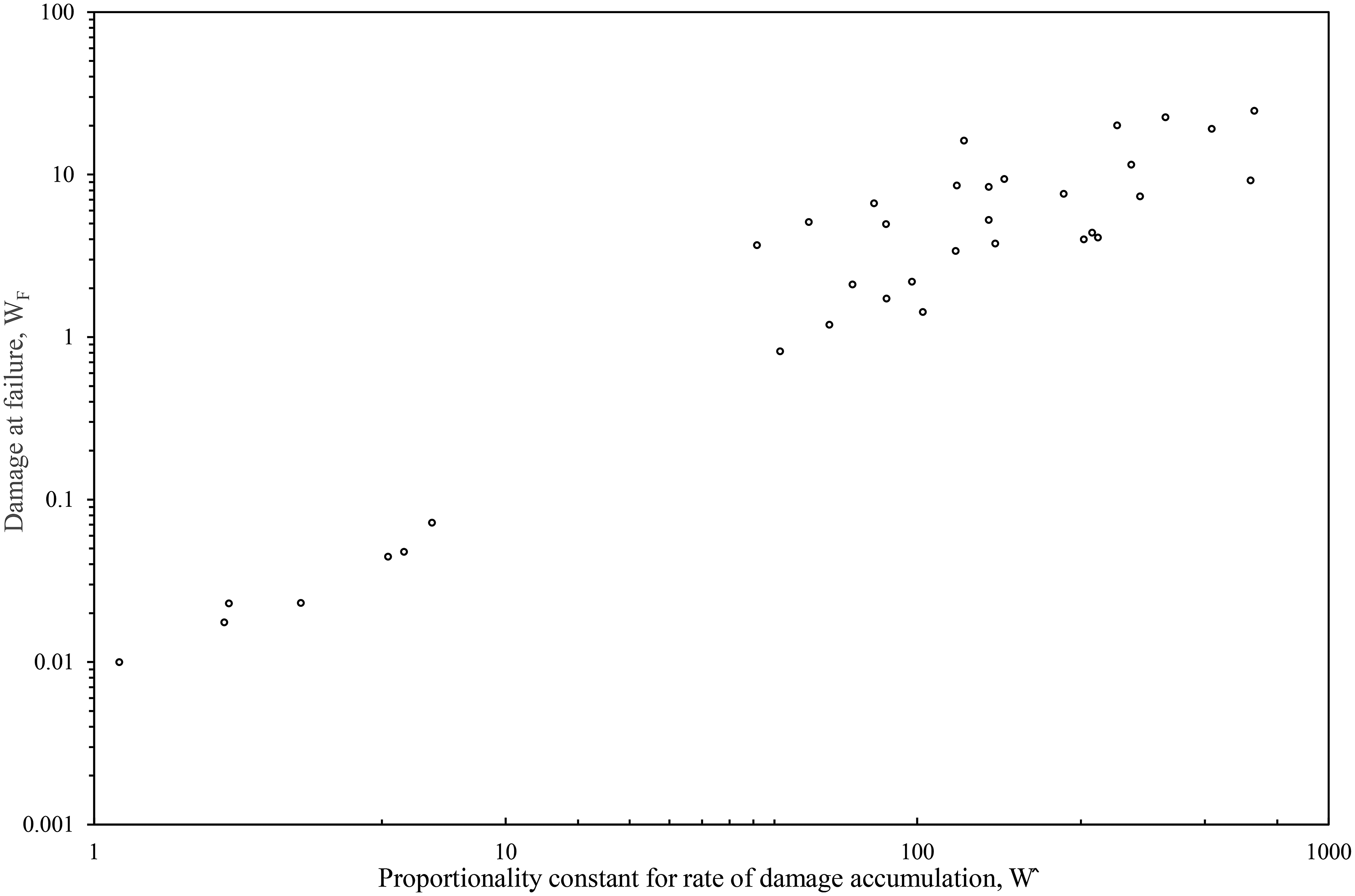
Relationship between damage at failure and rates of damage accumulation.
Monkman Grant relation
When applying Equation (1a) to all the experimental data outlined in the data section, ρ = 0.773 and M = 0.8048. There is however a lot of variation around this relation, with it explaining only around 93% of the variation in failure times. There appears to be some points that appear to be well above the fitted line and some that are well below the line which may be an indication that the Monkman-Grant constant M is not truly constant.
The following subsections demonstrate that the data in Figure 8 fit into three distinctly different groupings depending on the value for M2 and thus depending also on the tolerance to damage and the rate of damage accumulation. The statistical rational for such a grouping is provided in the failure time sub section below. Figure 9 plots the values for M2 as calculated using Equations (10, 12), against stress with the different symbols differentiating further with respect to temperature. Group 1a corresponds to test conditions producing M2 values below 0.73%, whilst Group 1c corresponds to test conditions producing M2 values above 1.7%. Group 1b corresponds to test conditions producing M2 values in between these two limiting values.
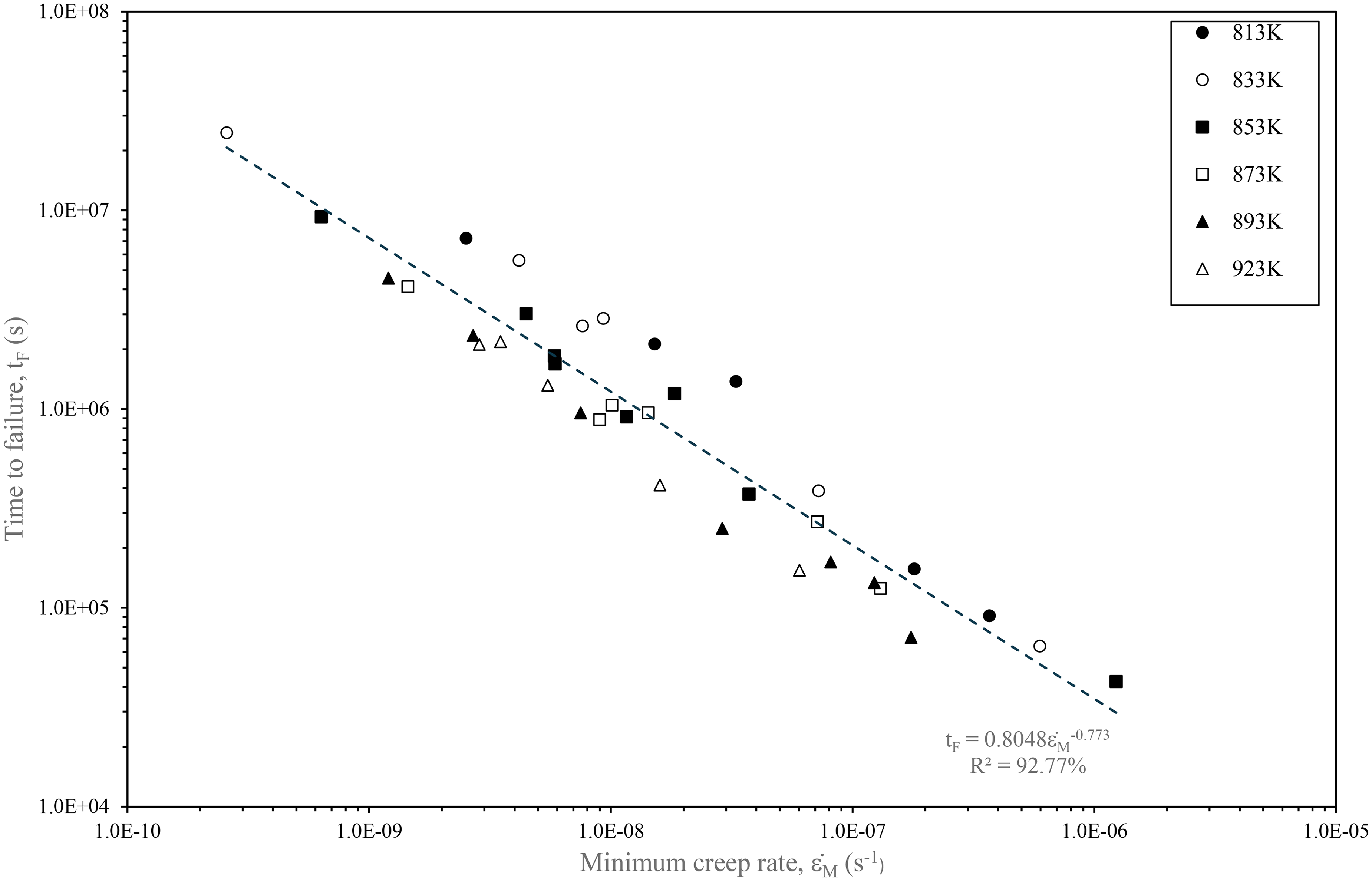
Variation in times to failure with measured minimum creep rates, together with the least squares regression line.
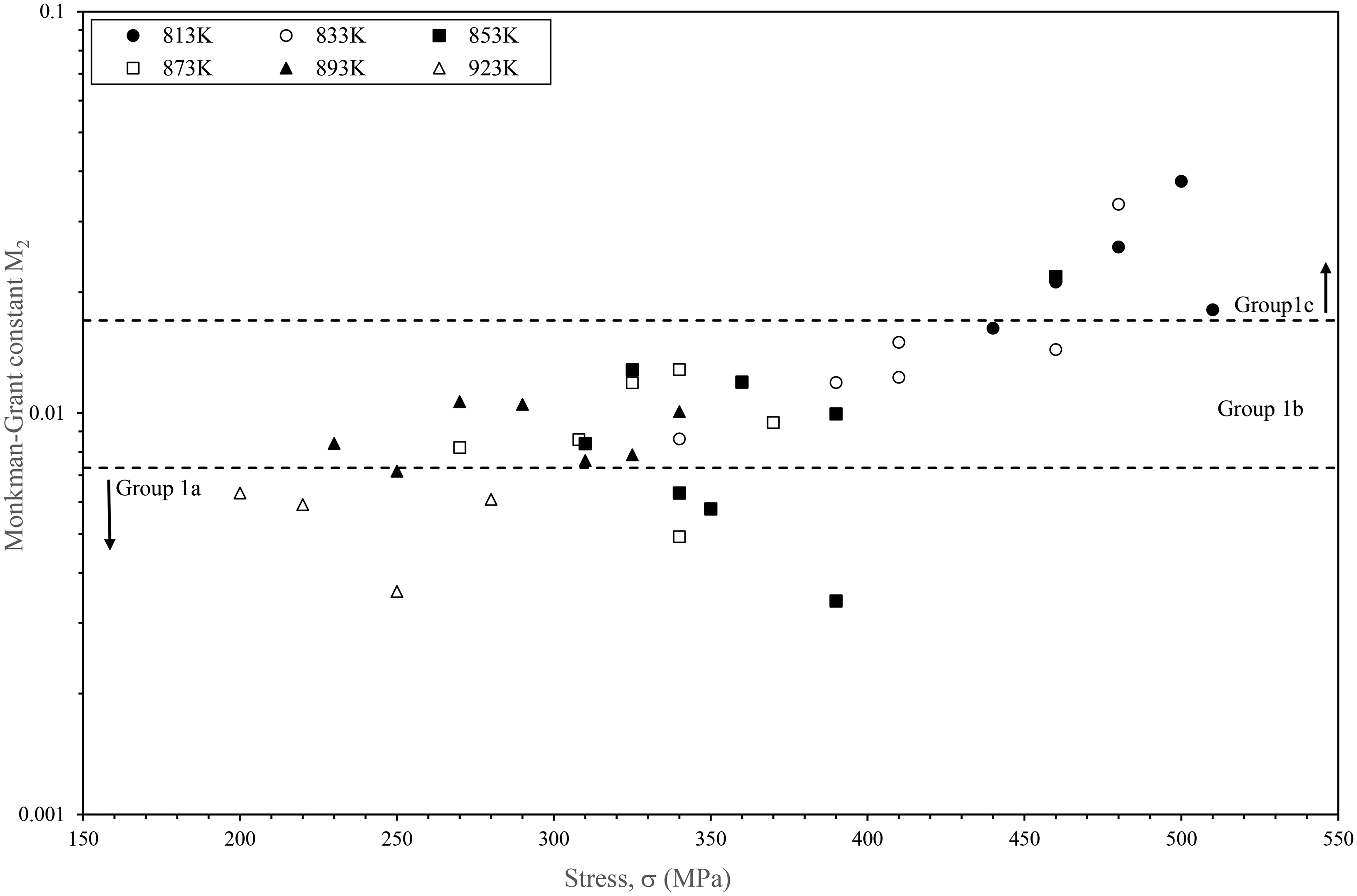
Variations in M2, as calculated using Equation (10), with stress and temperature.
Group 1c: Highest values for M2
Six data points make up this group and they correspond to the lowest three temperatures used in this test programme. They also correspond to the largest stress used at 833 K and 853 K and all but the lowest stress used at 813 K. Thus, relatively high M2 values are generated by high stresses at low temperatures. Figure 10 shows the creep curves corresponding to four of the six data points making up group 1c. The two creep curves obtained at 813 K (Figure 10(a), (b)) had almost identical levels of tertiary strain, but the specimen tested at 480 MPa, could tolerate nearly twice the amount of damage before failing. Yet both specimens had high M2 values, which can be explained by the fact the specimen tested at 480 MPa accumulated damage at almost twice the rate of the specimen test at 500 MPa. The specimen tested at 853 K (Figure 10(d)) could tolerate a large amount of damage before failing yet had an M2 value almost the same as the specimen tested at 480 MPa and 813 K (Figure 10(b)). This is because the damage in the specimen tested at 853 K had over twice the rate of damage accumulation than that experienced by the specimen tested at 480 MPa and 813 K.
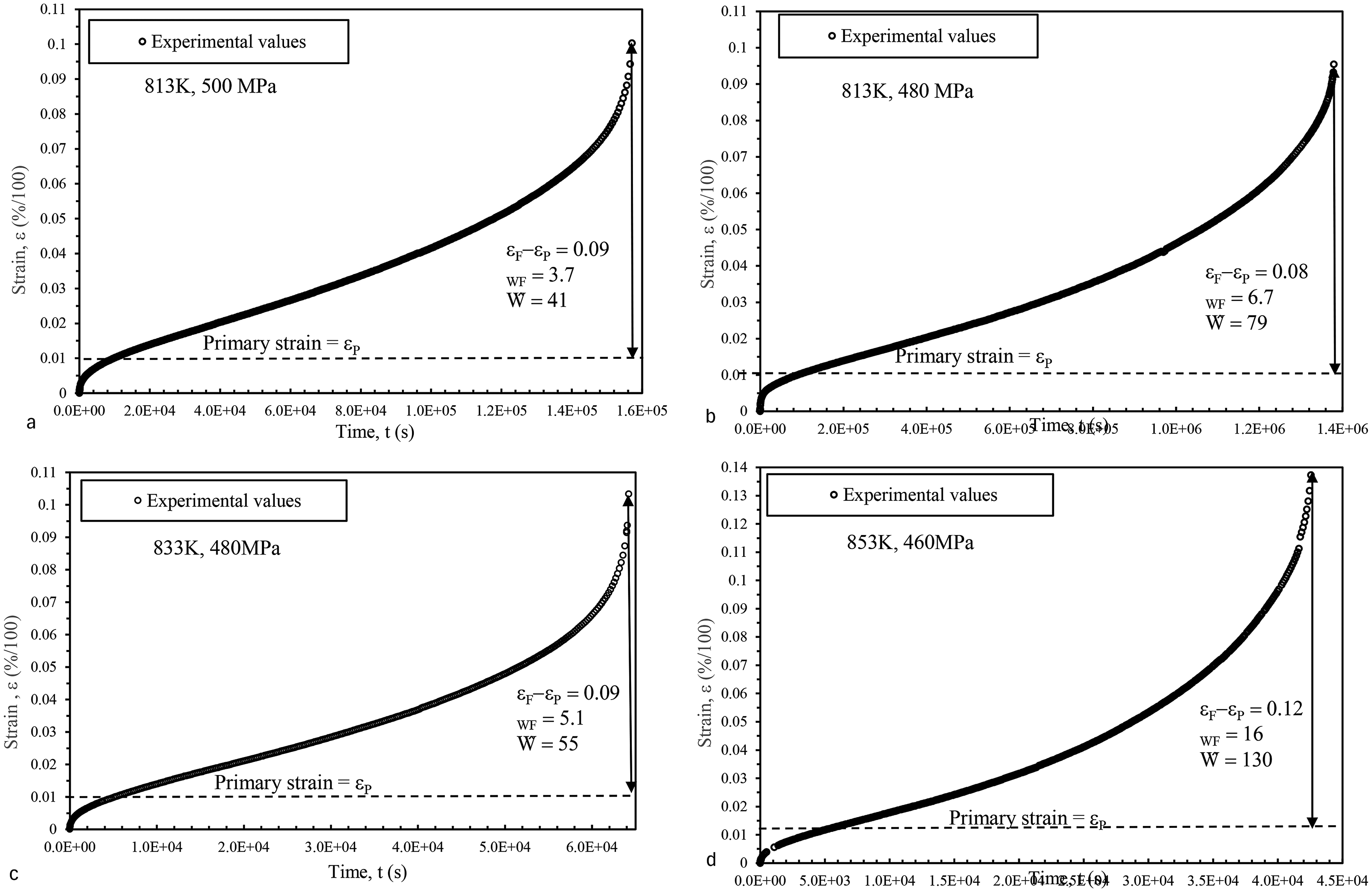
Creep curves with M2 values above 1.7%. a. at 813 K and 500 MPa, b. 813 K and 480 MPa, c. 833 K and 480 MPa and d. 853 K and 460 MPa.
Group 1a: Lowest M2 values
The low M2 values associated with this group are generated either by the two highest temperatures irrespective of stress, or at stresses below 390 MPa at a temperature of 853 K. This is because at 853 K M2 appears to be stress dependent but at the higher temperature of 923 K it is not. Figure 11 shows the creep curve corresponding to one data points making up group 1a. Now if we compare the Figure 11 with Figure 10(a), it becomes clear that these two test conditions result in similar tolerances to damage – (4.4 and 3.7). The specimen in Figure 10(a) has a much higher M2 value because it has a much lower rate of damage accumulation (41 compared to 266).
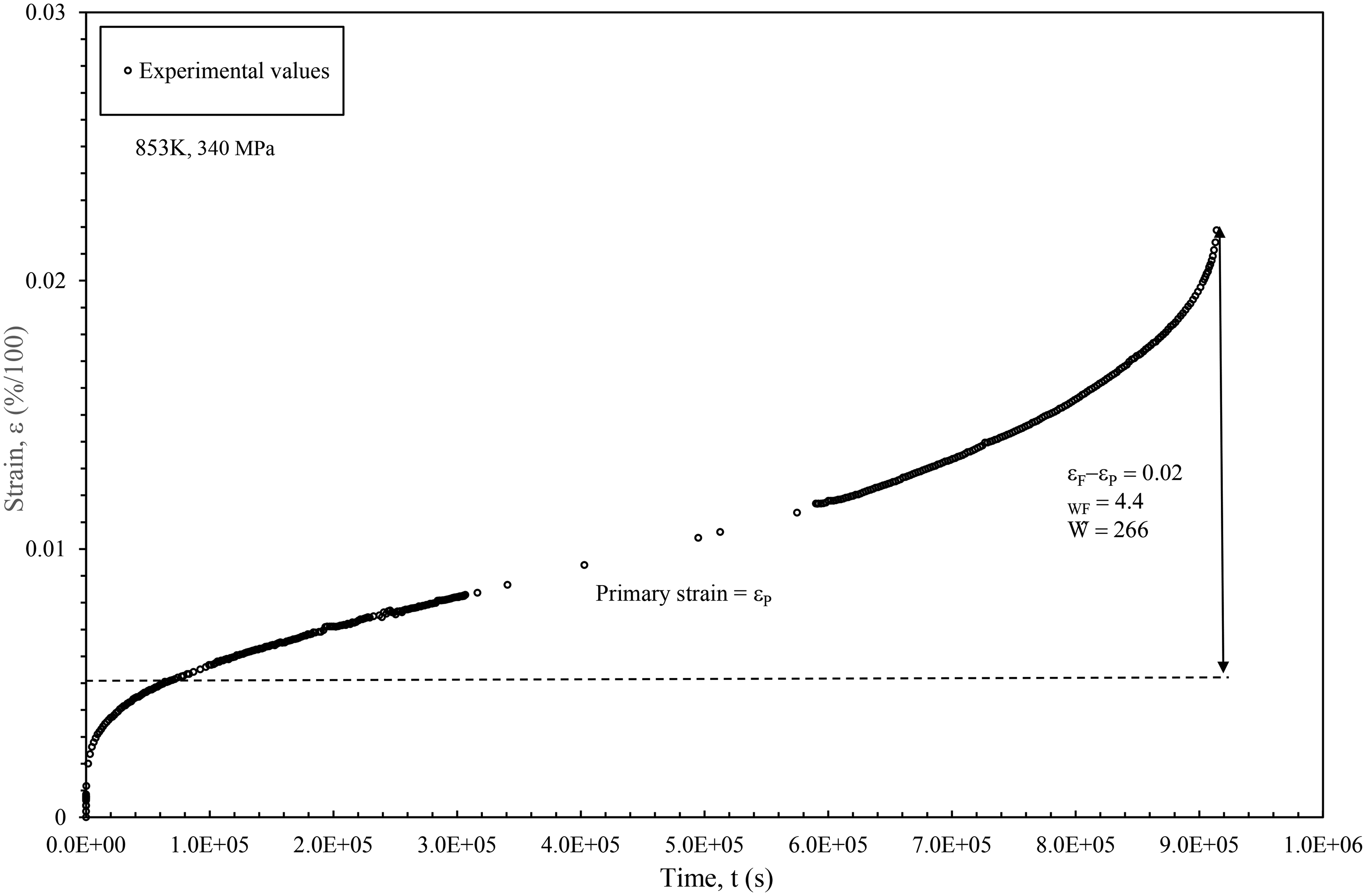
A creep curve with an M2 value below 0.95% obtained at 833 K and 390 MPa, and b. 853 K and 340 MPa.
The data in Figures 12 provides a further insight into the fundamental characteristics of the data points in this and the low M2 value group. Figure 12(b) plots values for M2 against WF and the data in groups 1a and 1c have broadly similar WF values – in group 1a WF is scattered around a mean value of 8, whilst in group 1c WF is scattered around a mean value of 20. Yet the data in group 1c have much higher M2 values compared to those in group 1a. Figure 12(a), which plots values for M2 against
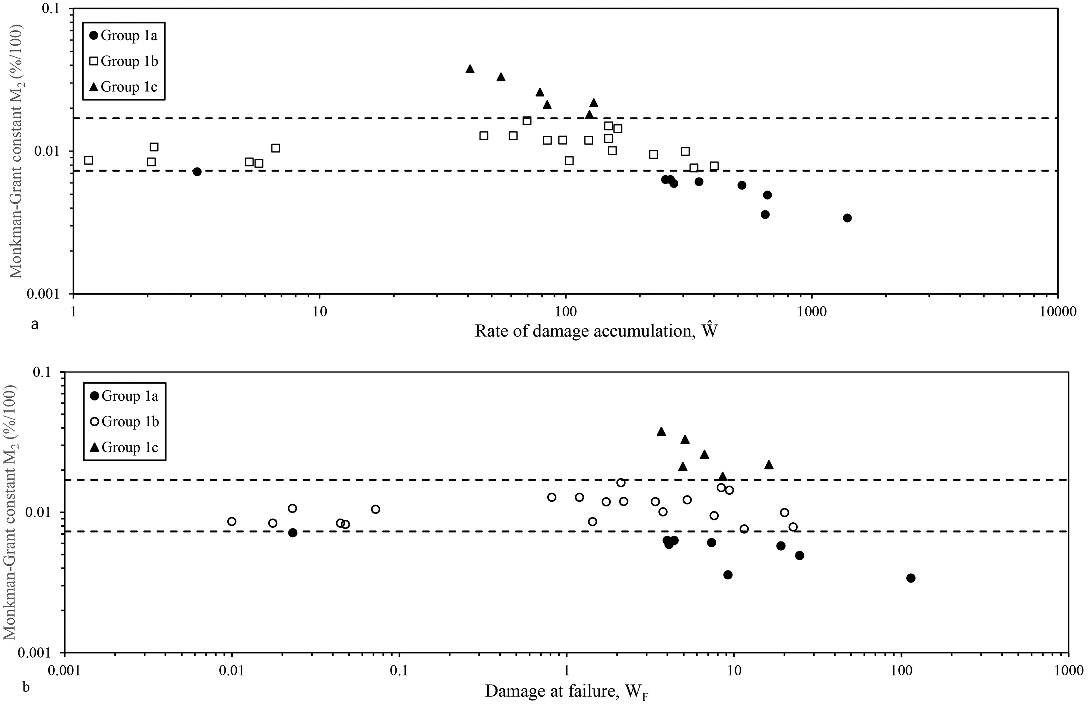
Variation in the Monkman-Grant constant M2 values with a. the proportionality constant for rates of damage accumulation
Thus, a high value for M2 is caused by a relatively high damage at failure and a relatively low rate of damage accumulation. Consequently, with a high tolerance to damage and a slow rate of damage accumulation the time to failure will be large, i.e., M2 is high so that at a given secondary creep rate failure times will be high in this group. Such characteristics are generated by high stresses at low temperatures. A low value for M2 is caused by a relatively high damage at failure with a relatively high rate of damage accumulation. Consequently, even though there is a high tolerance to damage, the higher rate of damage accumulation reduces the time taken to fail, i.e., M2 is low so that at a given secondary creep rate, failure times will be lower in this group. Such characteristics are generated by low stresses at a high temperature or moderately used stresses at a moderately used temperature.
Group 1b: Intermediate M2 values
The data points making up this group correspond to all but the highest temperature used −923 K – and stresses below 410 MPa. The specimen tested at the lower of these temperatures (Figure 13(a)) tolerated twice the amount of damage, but this damage occurred at only 15% of the rate experienced by the specimen tested at the higher temperature (Figure 13(b)), resulting in these two specimens having intermediate M2 values. Then if we compare the Figure 13(b) with Figure 10(b), it becomes clear that these two test conditions result in almost identical rates of damage accumulation – (79 and 84). The specimen in Figure 10(b) has a higher M2 value because it has higher tolerance to damage (6.7 compared to 1.7).
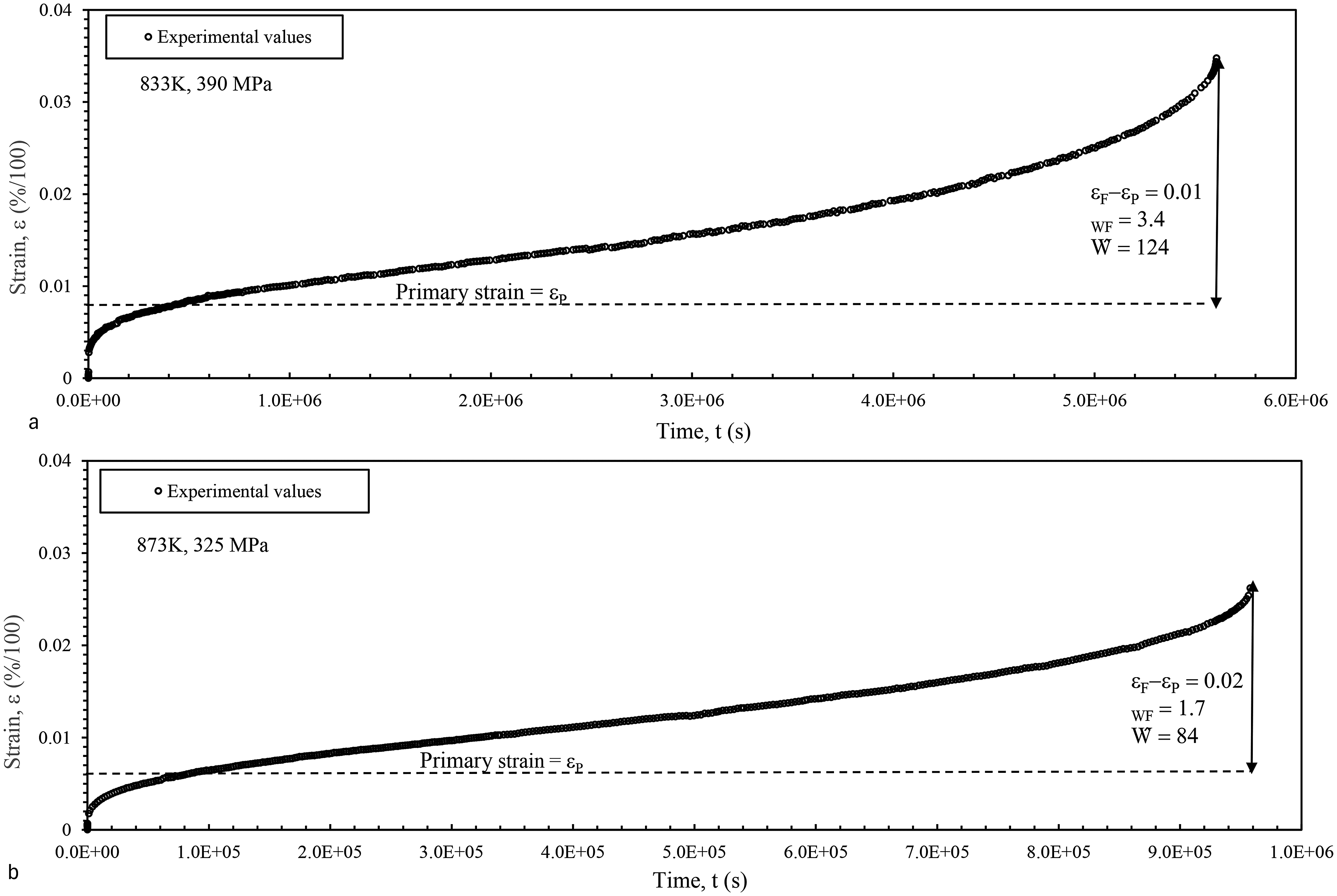
Some creep curves with M2 values below 1.7% but above 0.73%. a. at 833 K and 390 MPa, and b. 873 K and 325 MPa.
Figures 12 reveals there are two distinctly different creep characteristics generating the intermediate values for M2. The first group has values for WF that are like those in groups 1a and 1c, but these intermediate values for M2 are then generated by
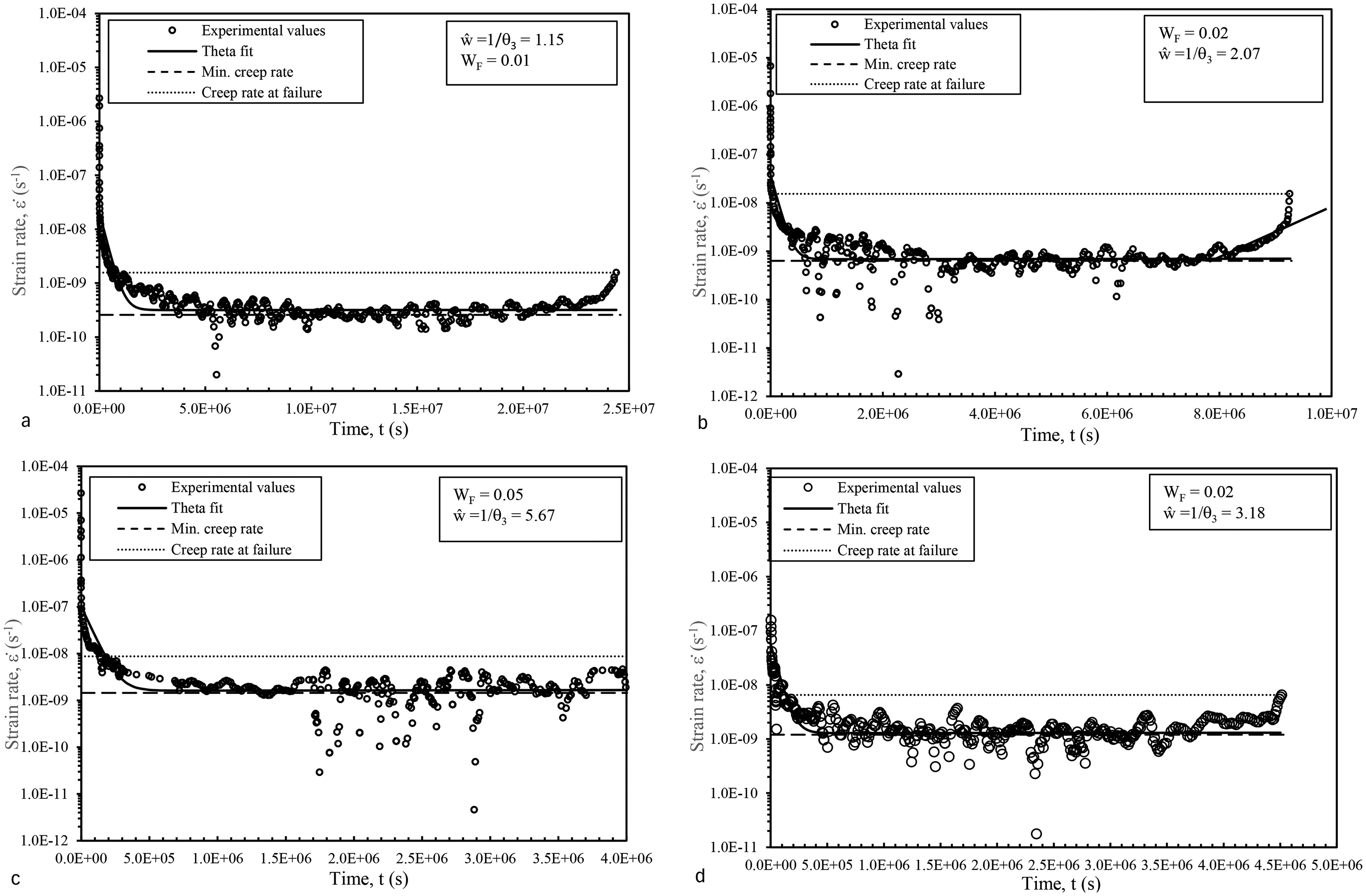
Variations in rates of creep with time for specimens tested at a. 833 K with 340 MPa, b. 853 K with 310 MPa, c. 873 K with 270 MPa and d.893 K with 250 MPa.
Figure 15 plots damage at failure against stress with a demarcation with respect to temperature also shown for all the data points making up group 1b. The very low amounts of damage at failure occur at the lowest stresses recorded at temperatures below 923 K. Further this move to very low amounts of damage, occurs at a stress of around 310 MPa. In the literature there is also some fractographic and microstructural evidence to support this pattern. Xu et. al. 24 found that at stresses below ∼340 MPa, dislocation-controlled creep dominates, precipitate coarsening is limited, and void nucleation is scarce—thus rupture occurs with minimal mesoscale damage and retains ductility. At higher stresses, these authors found that diffusional and grain-boundary driven damage accelerates. More specifically, Laves-phase coarsens, MX dissolves, void nucleation becomes widespread along boundaries, and damage localizes—leading to failure with significant damage signatures.

Variation of damage at failure with stress and temperature.
These authors also found that at stresses around 100–190 MPa, void densities are low and isolated with typical sizes ∼4–6 µm in diameter. Fractography revealed dimpled, ductile trans granular fracture with sparse cavities nucleated at coarse precipitates (e.g., Laves clusters). These void densities correspond to cavity area fractions well below ∼0.3%, indicating minimal damage at failure. Yan et. al. 25 found that at stresses of ≥ 300–400 MPa, void density and size escalate sharply. SEM fractography showed large clusters of cavities and cavity bands aligned along grain boundaries, typical of creeping along prior-austenite grain boundary zones. Fracture surfaces shift to mixed or intergranular modes, with visible cavity coalescence and secondary cracking.
Failure times
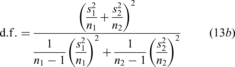
The statistical justification for the subgroupings shown above, is that the mean values for M2 in each group are statistically significantly different from each other. When using mean values, such statistical significance can be tested using the following t-value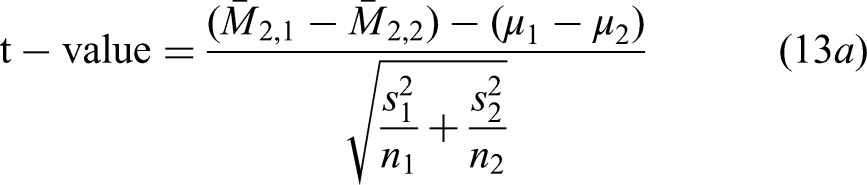
These t-values for mean comparisons are shown in the one but last column of Table 4. Thus, the t-value of −4.90 tests the null hypothesis that the difference between the true mean values for M2 in group 1a and group 1c are the same. Based on the t-value, the probability that this null hypothesis is true is 0.45%. So, at the 1% significance level, the mean value for M2 in these two groups are different, i.e., the negative value for the sample mean difference of (0.0055–0.0263) has not occurred by chance. Table 4 reveals that the three mean values are all statistically significantly different from each other at the 1% significance, so that the best fit lines in Figure 16 differ from each other in a statistically significant way.
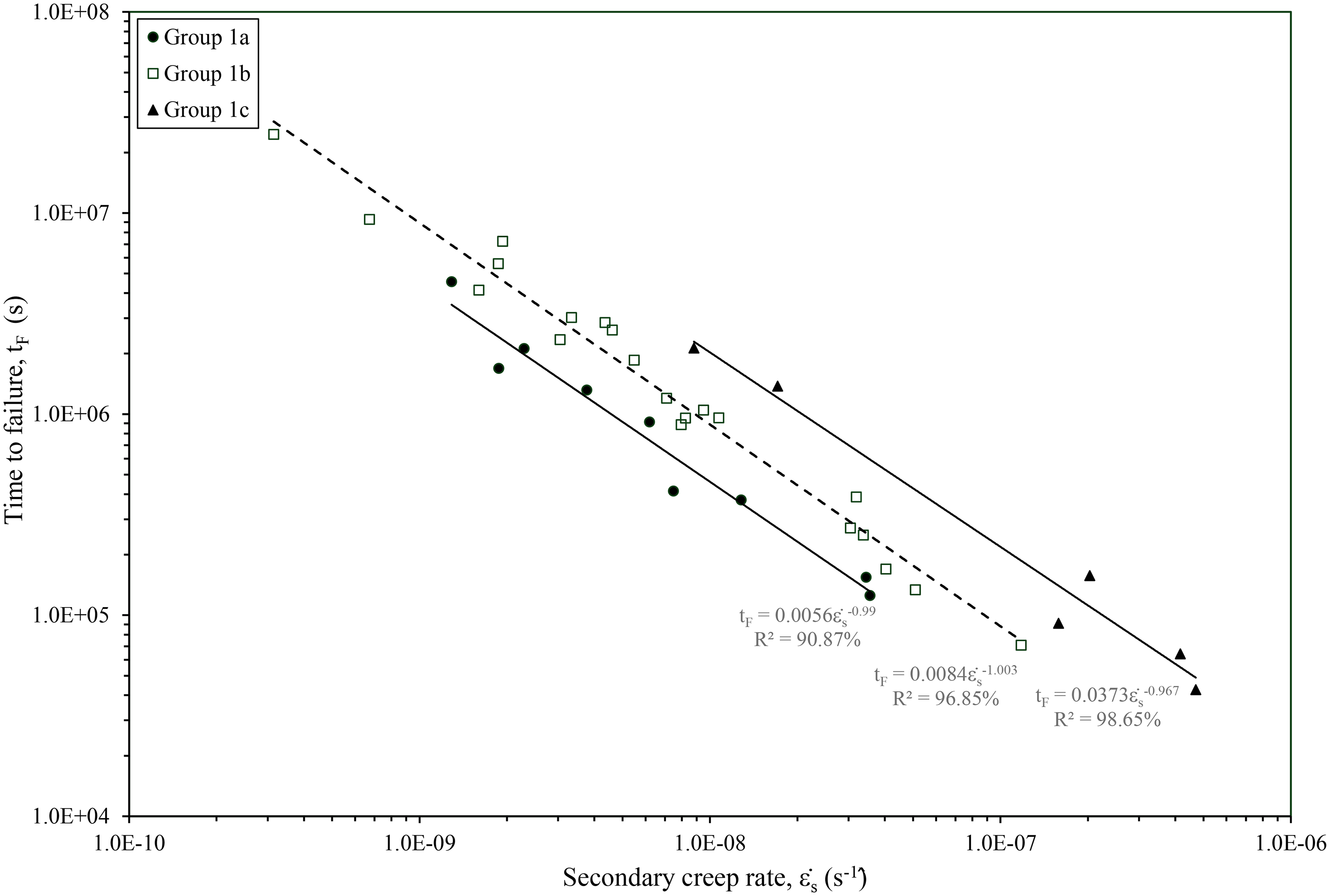
Variations in time to failure with the secondary creep rate, together with the estimated Monkman-Grant relation for each group of data.
Mean values for M2 in each grouping, together with tests for the statistical significance of differences between these means.
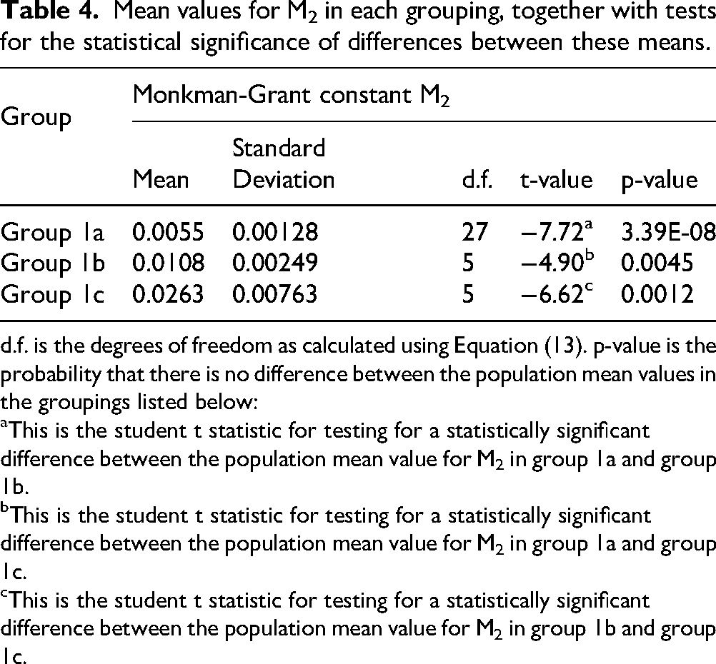
d.f. is the degrees of freedom as calculated using Equation (13). p-value is the probability that there is no difference between the population mean values in the groupings listed below:
This is the student t statistic for testing for a statistically significant difference between the population mean value for M2 in group 1a and group 1b.
This is the student t statistic for testing for a statistically significant difference between the population mean value for M2 in group 1a and group 1c.
This is the student t statistic for testing for a statistically significant difference between the population mean value for M2 in group 1b and group 1c.
Figure 16 shows the estimates made for the parameters of the Monkman-Grant relation of Equation (10) within each of the groupings identified above. The Monkman-Grant constant M2 increases from 0.56% in group 1a to 0.84% in group 1b and to 3.73% in group 1c. These significant differences take the form of a parallel shift as damage characteristics change. That is, ρ = 1 in all three groupings. Even in group 1c where ρ is estimated at 0.97, this is not significantly different from 1 – the p-value for the null hypothesis that the true value for ρ is 1 is 64.8%. There is therefore a very high probability that the true value for ρ is 1 (it would come out as 1 if there were many more data points available). The p-values for testing ρ = 1 in the other two groups are 55.5% for group 1a and 46.6% for group 1b. Thus, once account is taken for different amounts and rates of damage accumulation, the true value for ρ is 1, irrespective of these differences in damage. ρ = 1 is as predicted by the 4-θ methodology.
To further confirm the validity of the 4-θ Monkman-Grant relation, the data points of Figure 16 are replotted in Figure 17 according to Equation (10). The gradient of −0.995 of the regression line in Figure 17 corresponds to the exponent on
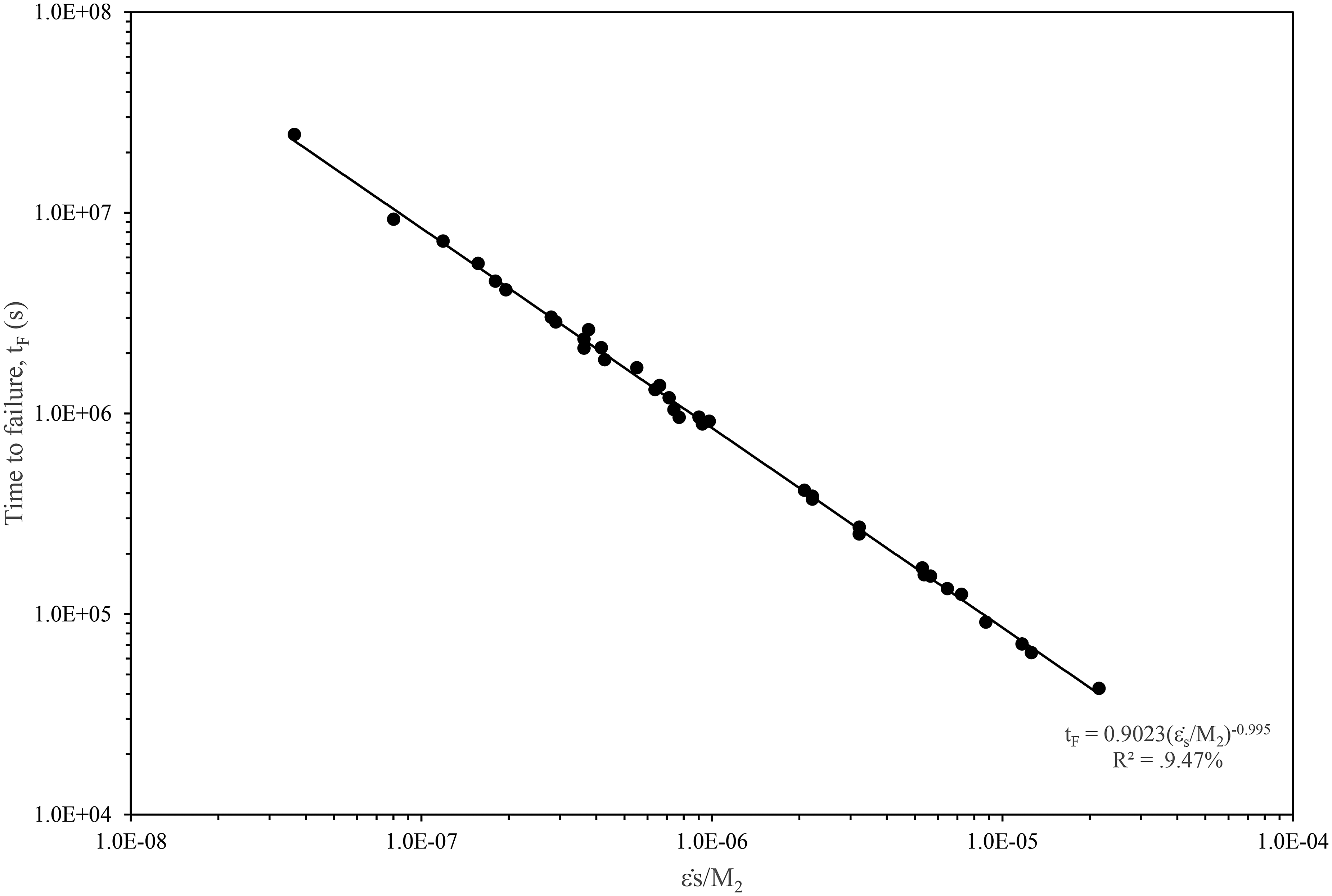
The modified 4-θ Monkman-Grant relation.
Conclusions
The Monkman-Grant relation offers the possibility of reducing the cost and length of the development cycle for new materials operating at high temperatures by using minimum creep rates that can be obtained relatively quickly even at low stresses. This paper used the 4-θ methodology to i. identify and explain the form of this relation in terms of creep mechanisms such as hardening, recover and damage and ii. to discover whether this form was compatible with long term creep life assessment. The 4-θ methodology suggests that the traditionally measured minimum creep rate should be replaced by the theoretical minimum creep rate measured as θ3θ4, It also predicts that the exponent on this secondary creep rate will equal −1. This methodology also predicted that the Monkman-Grant proportionality constant (M2) was positively related to the amount of strain during tertiary creep, positively related to the total amount of damage accumulated during this stage but negatively related to the rate at which damage accumulates. The methodology also suggested that the role played by primary creep in identifying the form of the Monkman-Grant relation was restricted to the determination of the theoretical secondary creep rate.
These predictions were confirmed by the data obtained on 12Cr-Mo-V-Nb steel. Without considering any of these causal variables, the exponent on the minimum creep rate was considerably different from the 4-θ prediction that it should equal −1 (−0.77). However, it was also found that the values for the Monkman-Grant proportionality constant (M2) fell into three well defined groupings depending on the amount of accumulated damage and the rate at which it occurred. Two of the groupings had similar amounts of damage at failure, but different rates of damage accumulation that split the data into low and high M2 values. It then turned out that within each such grouping, the exponent on the secondary creep rate equalled −1. The other grouping had rates of damage accumulation in between these two other groupings. However, this intermediate grouping also contained some results where both the amount of damage at failure and the rate at which it accumulated were very low (leading to an intermediate M2 value). What is interesting about this grouping is that this damage characteristic is typical of longer-term tests carried out at stresses much lower than those used in this paper and much closer to typical operating stresses for this material. As such the Monkman-Grant relation from this intermediate M2 grouping might be relevant for longer term life assessment based on early data on minimum creep rates at very low stress conditions. An interesting area for future research therefore is to study this possibility for reducing the development cycle for new materials in more detail.
Footnotes
Author contribution(s)
Funding
The author received no financial support for the research, authorship, and/or publication of this article.
Declaration of conflicting interests
The author declared no potential conflicts of interest with respect to the research, authorship, and/or publication of this article.
Appendix 1
Here a short confirmation that the derivative of M2 with respect to
Next, define u =
It needs to be shown that h(u) < 0 for all u> = 1, u ≠ 0 because ln(1 + u) is only defined for ln(1 + u) > 0. The derivative of h(u) with respect to u is
So, if u > 0 then
Appendix 2
Nomenclature for all the symbols
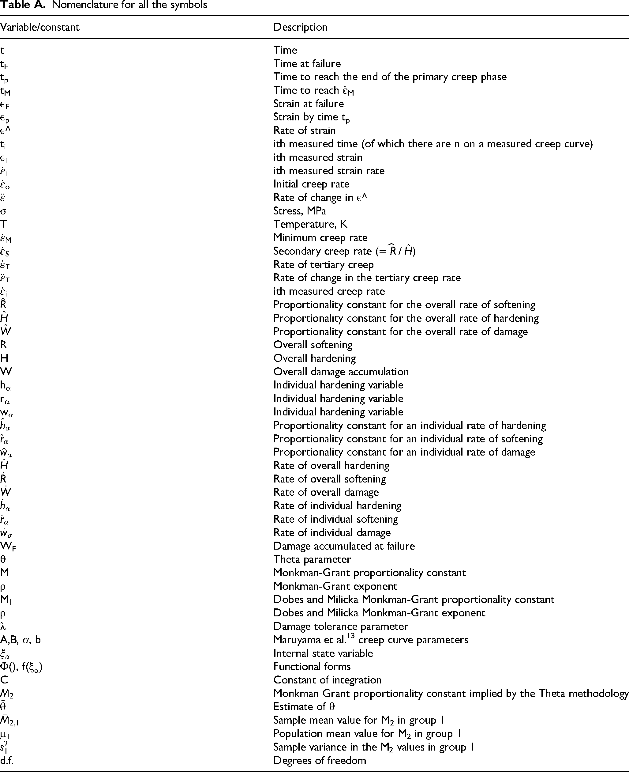
| Variable/constant | Description |
|---|---|
| t | Time |
| tF | Time at failure |
| tp | Time to reach the end of the primary creep phase |
| tM | Time to reach |
| εF | Strain at failure |
| εp | Strain by time tp |
| ε^ | Rate of strain |
| ti | ith measured time (of which there are n on a measured creep curve) |
| εi | ith measured strain |
| ith measured strain rate | |
| Initial creep rate | |
| Rate of change in ε^ | |
| σ | Stress, MPa |
| T | Temperature, K |
| Minimum creep rate | |
| Secondary creep rate (= ) | |
| Rate of tertiary creep | |
| Rate of change in the tertiary creep rate | |
| ith measured creep rate | |
| Proportionality constant for the overall rate of softening | |
| Proportionality constant for the overall rate of hardening | |
| Proportionality constant for the overall rate of damage | |
| R | Overall softening |
| H | Overall hardening |
| W | Overall damage accumulation |
| hα | Individual hardening variable |
| rα | Individual hardening variable |
| wα | Individual hardening variable |
| Proportionality constant for an individual rate of hardening | |
| Proportionality constant for an individual rate of softening | |
| Proportionality constant for an individual rate of damage | |
| Rate of overall hardening | |
| Rate of overall softening | |
| Rate of overall damage | |
| Rate of individual hardening | |
| Rate of individual softening | |
| Rate of individual damage | |
| WF | Damage accumulated at failure |
| θ | Theta parameter |
| M | Monkman-Grant proportionality constant |
| ρ | Monkman-Grant exponent |
| Dobes and Milicka Monkman-Grant proportionality constant | |
| ρ1 | Dobes and Milicka Monkman-Grant exponent |
| λ | Damage tolerance parameter |
| A,B, α, b | Maruyama et al. 13 creep curve parameters |
| Internal state variable | |
| Φ(), | Functional forms |
| C | Constant of integration |
| Monkman Grant proportionality constant implied by the Theta methodology | |
| Estimate of θ | |
| Sample mean value for M2 in group 1 | |
| μ1 | Population mean value for M2 in group 1 |
| Sample variance in the M2 values in group 1 | |
| d.f. | Degrees of freedom |