A statistical assessment of the equivalence between creep and hot tensile behaviour of 2.25Cr-1Mo steel

Abstract

It is important to be able to predict the creep life of materials used in power plants. Levi De Oliveira Bueno has suggested an equivalence between creep and high temperature tensile testing for 2.25Cr-1Mo steel. This offers the potential for reducing the development cycle for new materials designed to operate at ever higher temperatures. This paper reviews the literature to identify some suitable statistical tests for this equivalence. When applied to 2.25Cr-1Mo steel, it was found that this equivalence was only valid if the Monkman-Grant exponent equalled −1. However, this constraint was not accepted by the data based on the proposed statistical tests, and when this constraint was relaxed the equivalence between these different types of test data disappeared.

Introduction

Although complex stresses and temperatures are often encountered by materials used in power generation, design decisions are generally based on an “allowable” tensile creep strength. This strength is commonly taken to be 67% of the average stress (up to 1088 K). ¹ Currently, expensive testing lasting 12–15 years is required to determine the long-term strengths and lives. A reduction in this ‘materials development cycle’ was therefore defined as the No.1 priority in the 2007 UK Energy Materials – Strategic Research. ² With the aim of reducing this development cycle, a number of different approaches have been investigated. First, a new group of parametric creep models^3,4 have been developed in recent years that are characterised through their use of an S shaped curve to describe the relationship between the minimum creep rate and a normalised stress at a fixed temperature. These models have been shown to be stable with respect to time (test duration) and so have been reasonably successful^5–8 in predicting long term creep life from short term test data. Secondly, for materials where the Monkman- Grant ⁹ relation is stable over all test durations, a lifetime prediction can be made using measured minimum creep rates. As the minimum creep rate is reached well before rupture, this approach also offers the potential to reduce the length and cost of testing programs.

A hypothesis first put forward by Levi De Oliveira Bueno ¹⁰ in 2005 also offers the potential to reduce the time and costs of testing programs required for material development. This hypothesis was based around the similarities between a uniaxial creep test and a high temperature tensile test. A creep test involves subjecting a test specimen to a constant stress σ_c (or load) and high temperature (T) until it fails. During this time the specimen will strain at varying rates and the time at which the specimen fails t_cf and the minimum strain rate ${\dot{\epsilon }}_{\mathrm{mc}}$ are measured. A tensile test involves subjecting a test specimen to constant high temperature and a constant strain ${\dot{\epsilon }}_{\mathrm{ts}}$ until it fails. During this time the specimen will be subjected to a varying stress σ_ts (to ensure a constant strain rate) and the time at which the specimen fails t_ts and the maximum stress σ_ts (i.e., the ultimate tensile strength) are measured. The hypothesis made by Levi De Oliveira Bueno based on their results obtained on 2.25Cr-1Mo steel, was that i. σ_c was equivalent to σ_ts, ii. that t_cf was equivalent to t_ts and that iii. ${\dot{\epsilon }}_{\mathrm{mc}}$ was equivalent to ${\dot{\epsilon }}_{\mathrm{ts}}$ . In fact, Osgerby and Dyson ¹¹ demonstrated in an earlier paper, that the constant strain rate properties of a material are inextricably linked to its creep properties. Levi De Oliveira Bueno concluded that the Monkman-Grant constant was the same in the creep and tensile data sets which they took as evidence supporting the above hypothesis.

If this hypothesis is true, then a prediction of creep life at a typical operating condition can be quickly obtained. It involves conducting a number of tensile tests at different stain rates to estimate the MG relation in the tensile data set. These will all be cheap and very short-term tests. Then conduct just one creep test at the operating stress and temperature but discontinue it once the minimum creep rate has been observed. This will also be a short-term test in relation to how much time would be required for this specimen to fail. Finally, insert this minimum creep rate into the tensile MG relation for the creep strain to predict the creep failure time. This test program is quicker and cheaper than carrying out many creep tests at accelerated test conditions lasting several months.

But this identified similarity assumed that the Monkman-Grant (MG) exponent was equal to −1 (but as this paper demonstrates this value is larger than this within the creep data set used by Levi De Oliveira Bueno). That said, the Monkman-Grant relation provides an ideal framework within which to study the above hypothesis in more detail. This relation was first identified using data on the time to failure t_cf and the minimum creep rate ${\dot{\epsilon }}_{mc}$ both measured from uniaxial creep tests

$${\mathrm{t}}_{\mathrm{cf}}={\mathrm{M}}_{\mathrm{c}}({\dot{\epsilon }}_{\mathrm{mc}}{)}^{-1}$$

(1\rm a)

where M_c is material dependent. M_c can therefore be interpreted as the total strain experienced by a specimen if it crept at a strain rate of ${\dot{\epsilon }}_{\mathrm{mc}}$ . However, for many materials – especially high chrome steels ¹² and Nickel based super alloys ¹³ – it has been found that the following relation is more suitable

$${\mathrm{t}}_{\mathrm{cf}}={\mathrm{M}}_{\mathrm{c}}({\dot{\epsilon }}_{\mathrm{mc}}{)}^{-{\rho }_c}$$

(1\rm b)

where 0 < p_c< 1. This deviation (i.e., p_c< 1) from the simple MG relation of Eq. (1a) has been explained in a variety of different ways. Dobes and Milicka ¹⁴ attributed this deviation to variation in creep failure strain ε_cf

$${\displaystyle \frac{{\mathrm{t}}_{\mathrm{cf}}}{{\epsilon }_{\mathrm{cf}}}={\mathrm{M}}_{\mathrm{c}}({\dot{\epsilon }}_{\mathrm{mc}}{)}^{-1}}$$

(1\rm c)

Sklenicka et al. ¹⁵ found that for Grade 92 steel, the value of ρ_c in Eq. (1b) was 0.88, but when ${\mathrm{t}}_{\mathrm{cf}}$ is replaced with $\frac{{\mathrm{t}}_{\mathrm{cf}}}{{\epsilon }_{\mathrm{cf}}}$ in Eq. (1b) the value for ρ_c increased to 0.96. In contrast to this, Abe ¹⁶ attributed this deviation to accelerating creep strain rates during tertiary creep

$${\displaystyle \frac{\mathrm{dln}({\dot{\epsilon }}_c)}{\mathrm{d}{\epsilon }_c}{\mathrm{t}}_{\mathrm{cf}}=\left({\displaystyle \frac{{\mathrm{t}}_{\mathrm{cf}}}{({\mathrm{t}}_{\mathrm{cf}}-{\mathrm{t}}_{\mathrm{m}})}}\right)({\dot{\epsilon }}_{\mathrm{mc}}{)}^{-1}}$$

(1\rm d)

where t_m is the time taken to reach the minimum creep rate, ε_c is the creep strain and $\dot{\epsilon }$ _c the creep strain rate. However, when applied to 9Cr-1 W steel, Abe obtained a value for ρ_c that was less than 1.

The Levi De Oliveira Bueno hypothesis can be tested within the MG framework, by assuming the MG relation of Eq. (1b) applies to the tensile test results as well

$$t_{ts}=M_{ts}{\dot{\epsilon }}_{ts}^{-{\rho }_{ts}}$$

(1\rm e)

where t_ts is the time it takes for the varying stress in a tensile test to reach its maximum (i.e., the tensile stress) and ${\dot{\epsilon }}_{ts}$ is the constant strain under which this tensile test was carried out. If parts ii and iii of the Levi De Oliveira Bueno hypothesis are true, then this will only be so if $M_c$ = $M_{ts}$ and if ρ_c= ρ_ts. When this is the case, data pairings of (t_ts, ${\dot{\epsilon }}_{ts}$ ) and (t_c, ${\dot{\epsilon }}_c)$ will all fall on the same curve implying that t_cf and t_ts are equivalent and that ${\dot{\epsilon }}_{\mathrm{mc}}$ and ${\dot{\epsilon }}_{\mathrm{ts}}$ are equivalent. The hypothesis made by Levi De Oliveira Bueno can therefore be expressed in terms of parameter restrictions within the MG relation. This enables some standard statistical tests to be used.

The Levi De Oliveira Bueno hypothesis is an interesting hypothesis, because if true, it would enable a reliable creep life prediction at design conditions to be made from very short term (minutes) high temperature tensile tests. This would remove the need for even accelerated creep testing. The aim of this paper it to apply statistical test to this hypothesis within the MG framework using the data of Levi De Oliveira Bueno ¹⁰ on 2.25Cr- 1Mo steel. To achieve this aim, the paper is structured as follows. The following section describes this data set in a bit more detail. This is followed by a section outlining some statistical tests for this hypothesis (with much of the statistical theory confined to an appendix). The penultimate section presents the results from applying these statistical tests and finally a conclusion section outlines some proposed areas for future work.

The data

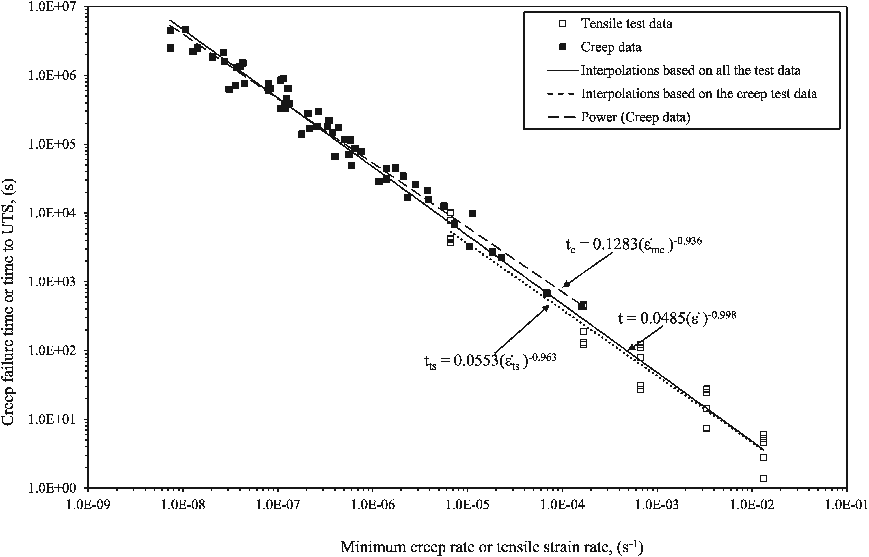
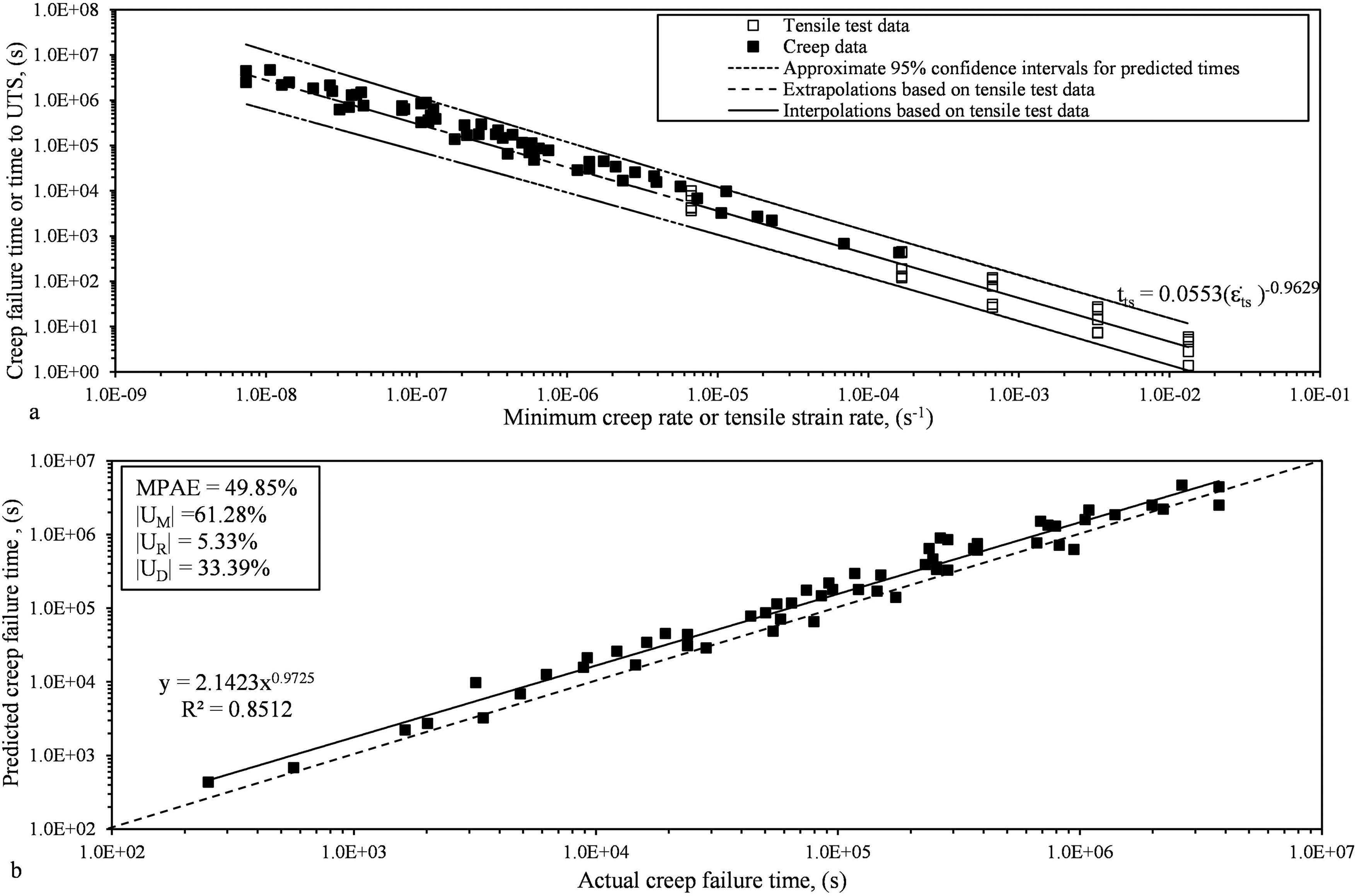
High temperature tensile and creep properties for 2.25Cr-1Mo steel have been published by Bueno & Sobrinho. ¹⁰ The steel they used for testing was supplied in plate form with 25.4 mm thickness according to ASTM A 387, Grade 22 and in the normalized and tempered condition with the following chemical composition: Fe – 2.09Cr – 1.08Mo – 0.097C – 0.32Si – 0.50Mn – 0.007P – 0.002S – 0.03Ni – 0.01Cu – 0.05Al. Metallographic analysis carried out by these researchers indicated the presence of 30% bainite and 70% ferrite. Test specimens were extracted from the rolling direction and had a gauge length of 25 mm and an initial diameter of 6.25 mm. High temperature tensile testing was carried out on a servo-hydraulic 8802 model INSTRON machine using five different temperatures ranging from 873 K to 973 K and at five different constant strain rates ranging from 6.67 × 10⁻⁶ s⁻¹ up to 0.01 s⁻¹. Figure 1 plots the constant strain rates against the time taken to reach the ultimate tensile strength in all these high temperature tensile tests (open squares).

Figure 1.

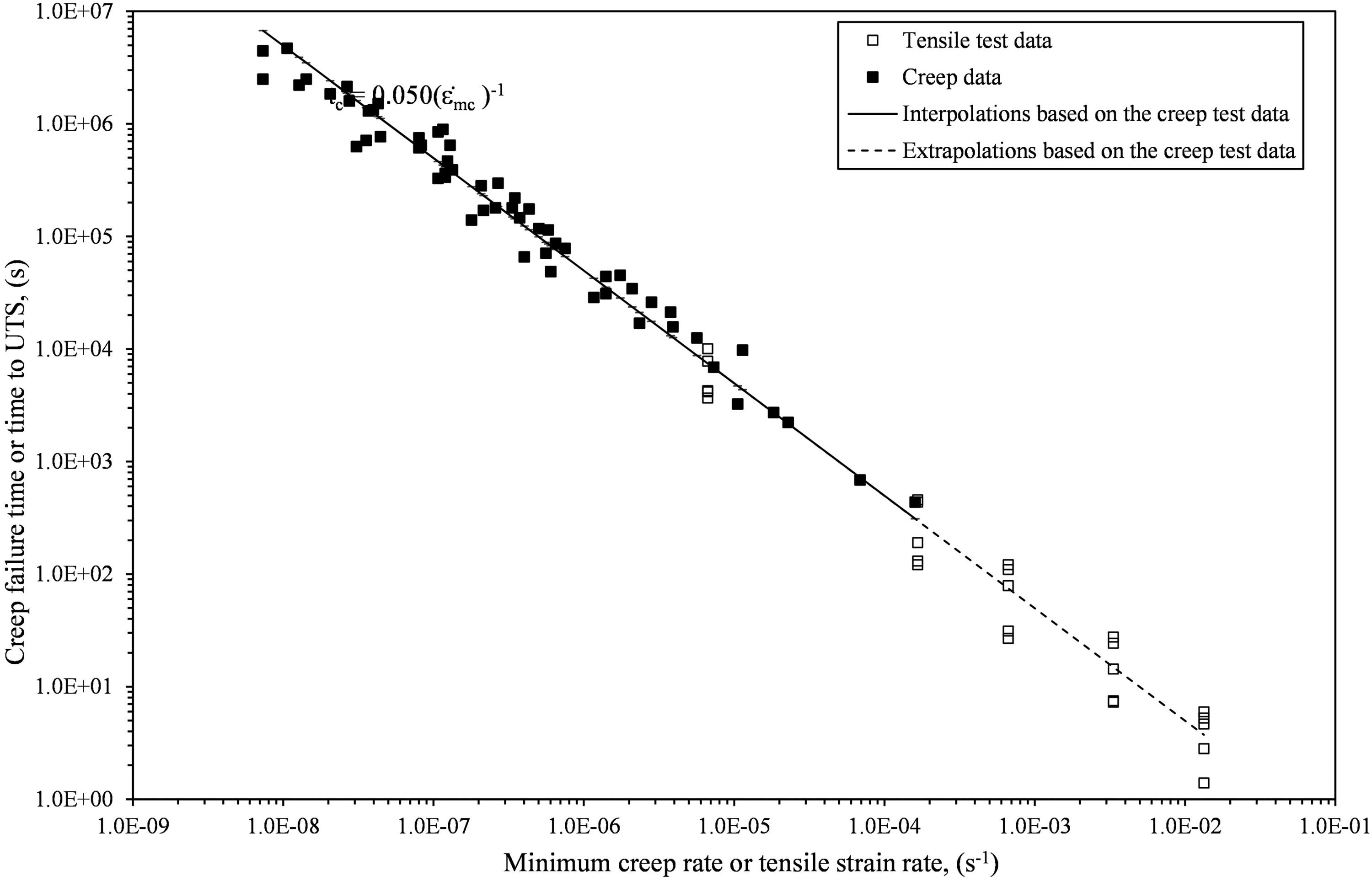
Variation of the minimum creep rate with the rupture time in creep test data, plotted together with the strain rate and time to occurrence of the ultimate tensile stress (UTS) in the constant strain rate tensile tests. Straight lines refer to the least squares estimates of the MG relation in the creep (long dashed), tensile (short dashed) and combined (sold line) test data sets.

The creep tests carried out by Bueno & Sobrinho were at constant load, according to ASTM E139, ¹⁷ using a set of 10 creep machines model STM-MF 1000. (Further information about this equipment and testing techniques appears in. ¹⁸ The elongation of the specimens was followed with creep extensometers having Transtek LVDT transducers - model DCDT 0243-000. The readings from the transducers were collected by a Fluke Data Logger, model Hydra 2635A series II, using scan rates varying from 6 readings/min to 6 readings/h. The creep tests were carried out at nine temperatures levels, ranging from 773 K to 973 K, covering nineteen levels of applied load, varying from 34 MPa to 448 MPa. The resulting minimum creep rates and rupture lives are also shown in Figure 1 with failure times ranging from 0.12 to about 1300 h (closed squares). It can be seen that there seems to be more variability in the high temperature tensile tests data set.

Methodology

In Figure 1, the MG relation is applied separately to the creep test data and the tensile test datasets, together with the fit to the pooled data set. A difference is observed in the values for the MG constant and exponents in each data set, but what is required is a test that assesses whether these observed differences in the parameters of the MG relation are statistically significant, i.e., that these observed differences have not occurred by chance.

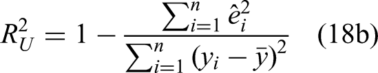
Testing single parameter restrictions when the Monkman-Grant exponent is 1

If the Monkman-Grant exponent term is unity, it can be expressed as follows for both the creep and tensile test results

$${\mathrm{t}}_{\mathrm{cf}}({\dot{\epsilon }}_{\mathrm{mc}})={\mathrm{M}}_{\mathrm{c}}$$

(2\rm a)

$$t_{ts}({\dot{\epsilon }}_{\mathrm{ts}})=M_{ts}$$

(2\rm b)

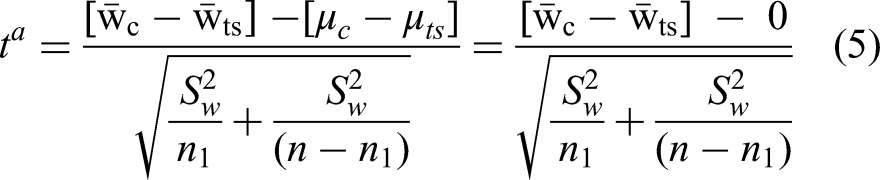
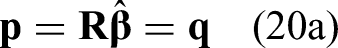
If parts ii and iii of the Levi De Oliveira Bueno hypotheses are true, then this will only be so if $M_c$ = $M_{ts}$ . So, one approach to testing this parameter restriction is to test whether the mean values for M_c and M_ts are the same. Existing tests for differences in population means are heavily reliant on use of the normal distribution or the central limit theorem, yet it is well established that creep failure times and minimum creep rates have long tailed distributions. Taking natural logs can transform such variables into normal variates – for example if t_cf has a long-tailed log normal distribution, ln(t_cf) will be normally distributed. There is therefore good reason for expressing the above MG equations in natural logs

$$\ln ({\mathrm{t}}_{\mathrm{cf}})+\ln ({\dot{\epsilon }}_{\mathrm{mc}})=\ln ({\mathrm{M}}_{\mathrm{c}})$$

(3\rm a)

$$\ln ({\mathrm{t}}_{\mathrm{ts}})+\ln ({\dot{\epsilon }}_{\mathrm{ts}})=\ln ({\mathrm{M}}_{\mathrm{ts}})$$

(3\rm b)

Let μ_c be the population or true mean for $\ln ({\mathrm{M}}_{\mathrm{c}})$ and μ_ts be the population or true mean for $\ln ({\mathrm{M}}_{\mathrm{ts}})$ . A test of the null hypothesis H_o: μ_c - μ_ts= 0 is then one way to test the Levi De Oliveira Bueno hypothesis. To conduct such a test, two samples of data are required. The first is the tensile test data set to be made up of i = 1 to n₁ measurements on $\ln ({\mathrm{t}}_{\mathrm{ts}})\mathrm{and}\ln ({\dot{\epsilon }}_{ts})$ and the second is a creep test data set to be made up of i = n₁+ 1 to n measurements on $\ln ({\mathrm{t}}_{\mathrm{cf}})\mathrm{and}\ln ({\dot{\epsilon }}_{\mathrm{mc}})$ (such that n > n₁). Then let the variables y_i= ln(t_cf)_i and x_1i= ln( ${\dot{\epsilon }}_{ts}$ )_i when n ≤ i > n_1, but y_i= ln(t_ts) and x_1i= ln( ${\dot{\epsilon }}_{ts})$ _i when i ≤ n₁. Eqs. (3) can then be written as

$${\mathrm{w}}_{\mathrm{ts},\mathrm{i}}={\mathrm{y}}_{\mathrm{i}}+{\mathrm{x}}_{\mathrm{i}}=\ln ({\mathrm{M}}_{\mathrm{ts}}{)}_i\mathrm{i}=1\mathrm{to}{\mathrm{n}}_1$$

(4\rm a)

$${\mathrm{w}}_{\mathrm{c},\mathrm{i}}={\mathrm{y}}_{\mathrm{i}}+{\mathrm{x}}_{\mathrm{i}}=\ln ({\mathrm{M}}_{\mathrm{c}}{)}_{\mathrm{i}}\mathrm{i}=1+{\mathrm{n}}_1\mathrm{to}\mathrm{n}$$

(4\rm b)

Section A of the appendix shows that if the variance in each test data set are the same, σ²_c= σ²_ts= σ²_w, and if w_ts,i and w_c,i are both normally distributed (if not then the central limit theorem will ensure ${\overline{\mathrm{w}}}_{\mathrm{c}},{\overline{\mathrm{w}}}_{\mathrm{ts}}$ will still be normally if calculated from a large sample) then the following t statistic can be used to test the null hypothesis H_o: μ_c - μ_ts= 0

$$t^a={\displaystyle \frac{[{\overline{\mathrm{w}}}_{\mathrm{c}}-{\overline{\mathrm{w}}}_{\mathrm{ts}}\left]-\right[{\mu }_c-{\mu }_{ts}]}{\sqrt{{\displaystyle \frac{S_w^2}{n_1}+{\displaystyle \frac{S_w^2}{(n-n_1)}}}}}={\displaystyle \frac{[{\overline{\mathrm{w}}}_{\mathrm{c}}-{\overline{\mathrm{w}}}_{\mathrm{ts}}]-0}{\sqrt{{\displaystyle \frac{S_w^2}{n_1}+{\displaystyle \frac{S_w^2}{(n-n_1)}}}}}}}$$

(5)

because if the null is true, t^a has a student t distribution with n – 2 degrees of freedom. ${\overline{\mathrm{w}}}_{\mathrm{c}},{\overline{\mathrm{w}}}_{\mathrm{ts}}$ are the sample means for w_c and w_ts respectively, and s²_w is the sample estimate of the common variance σ²_w (Appendix A gives the formulas for ${\overline{\mathrm{w}}}_{\mathrm{c}},{\overline{\mathrm{w}}}_{\mathrm{ts}}$ and s²_w)_.

Values for the probability of observing various values for t^a have been tabulated. For example, there is a 5% chance of observing a t^a value outside the range −2.23 to +2.23 when the degrees of freedom equals 10. If a calculated value for |t^a| from Eq. (5) then exceeds 2.23 it can be said that the chances of getting such a value is less than 5%. As this |t^a| value was calculated under the assumption that that ${\mu }_c-{\mu }_{ts}$  = 0, it follows that there is also less than a 5% chance that the true value for ${\mu }_c-{\mu }_{ts}$  = 0. The decision rule is to reject the null hypothesis whenever |t^a| > |t_α/2,n−2| as this runs only a α% chance of being wrong in that rejection decision. |t_α/2,n−2| is called the critical value for t. Alternatively, the p-value is the probability of observing |t^a| or more, and so is equivalent to the probability of the null hypothesis being true. The null hypothesis is then rejected when p-value < α%.

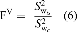
The normality assumption required to hold for the above test is almost guaranteed by the central limit theorem that states that the distribution for a sample mean tends to a normal distribution as the sample size from which it's calculated tends to infinity and from the fact that linear combinations of normal variables $[{\overline{\mathrm{w}}}_{\mathrm{c}}-{\overline{\mathrm{w}}}_{\mathrm{ts}}]$ are also normal. The approximation to normality is excellent in samples of size 30 or more. The assumption that σ²_wc= σ²_wts= σ²_w can be tested using the ratio of the sample estimates of these variances

$${\mathrm{F}}^{\mathrm{V}}={\displaystyle \frac{S_{{\mathrm{w}}_{ts}}^2}{S_{{\mathrm{w}}_c}^2}}$$

(6)

which under the null hypothesis that σ²_c= σ²_ts has an F distribution with n - n₁ - 1 and n₁ −1 degrees of freedom (as the variances are chi squared distributed and the ratio of two chi square variables has an F distribution). Consequently, if the value for ${\mathrm{F}}^{\mathrm{V}}$ in Eq. (6) exceeds F_α, then the observed value for F^V has less than a α% chance of being observed. If such a value is then actually observed, this can only then be explained by ${\mathrm{F}}^{\mathrm{V}}$ not having an F distribution – which will only be so if the null hypothesis is not true. Here F_α is the value for F^V such that there is only a probability of α that this value or more will be observed. So, the null hypothesis is rejected only if F^V> F_α, i.e., when the chances of the null hypothesis being true have dropped so low that it cannot be entertained as a realistic possibility.

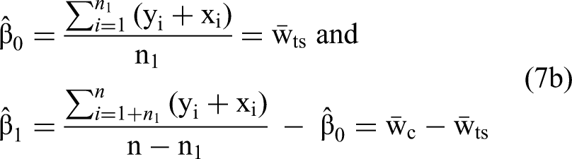
Another reason for testing differences between log means, is that taking logs linearises non-linear equations like the MG relation. This then enables the technique of linear least squares to be used to test the Levi De Oliveira Bueno when the MG exponent is not unity, i.e., when the above means difference test is no longer suitable. If the variable I_i= 0 when i ≤ n₁ but I_i= 1 when i > n₁, then the value for I_i distinguishes results from the creep and tensile tests. Given this, it is possible to combine Eqs. (4) into a single equation where β₀= ln(M_ts) and β₀+ β₁= ln(M_c) in

$${\mathrm{y}}_{\mathrm{i}}+{\mathrm{x}}_{\mathrm{i}}={\beta }_{\mathrm{o}}+{\beta }_1{\mathrm{I}}_{\mathrm{i}}+{\mathrm{v}}_{\mathrm{i}}\mathrm{for}\mathrm{i}=1\mathrm{to}\mathrm{n}$$

(7\rm a)

Consequently, testing the Levi De Oliveira Bueno hypothesis boils down to testing the hypothesis that β₁= 0. The variable v_i in Eq. (7a) represents the scatter that is measured around the regression line and reflects the stochastic nature of creep and tensile testing. The least squares procedure is one that choses values for β_o and β₁ that minimises the Σv²_i, where the sum is over all n observations. The solution to this optimisation problem is

$$\begin{array}{rl}& {\hat{\beta }}_0={\displaystyle \frac{{\sum }_{i=1}^{n_1}({\mathrm{y}}_{\mathrm{i}}+{\mathrm{x}}_{\mathrm{i}})}{{\mathrm{n}}_1}={\overline{\mathrm{w}}}_{\mathrm{ts}}\mathrm{and}}\\ & {\hat{\beta }}_1={\displaystyle \frac{{\sum }_{i=1+n_1}^n({\mathrm{y}}_{\mathrm{i}}+{\mathrm{x}}_{\mathrm{i}})}{\mathrm{n}-{\mathrm{n}}_1}-{\hat{\beta }}_0={\overline{\mathrm{w}}}_{\mathrm{c}}-{\overline{\mathrm{w}}}_{\mathrm{ts}}}\end{array}$$

(7\rm b)

where the hat denotes that these are estimates of the true population values β_o and β₁. If the v_i are assumed to be normally distributed and if the variance of the residuals v_i is a constant (i.e., the same value in the creep and tensile data sets) equal to σ²_v, then

$$t^b={\displaystyle \frac{{\hat{\beta }}_{\mathrm{j}}-{\beta }_{\mathrm{j}}}{\sqrt{{\mathrm{s}}_{\mathrm{v}}^2\left[{\displaystyle \frac{1}{{\mathrm{n}}_1}+{\displaystyle \frac{1}{(n-n_1)}}}\right]}}\mathrm{j}=1\mathrm{to}2}$$

(8\rm a)

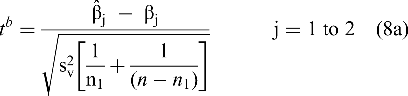
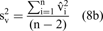
has a student t distribution with n - 2 degrees of freedom. s²_v is the following unbiased estimate of σ²v

$${\mathrm{s}}_{\mathrm{v}}^2={\displaystyle \frac{{\sum }_{\mathrm{i}=1}^{\mathrm{n}}{\hat{\mathrm{v}}}_{\mathrm{i}}^2}{(\mathrm{n}-2)}}$$

(8\rm b)

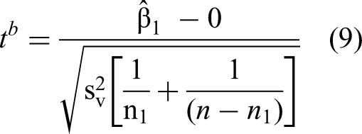
where the ${\hat{\mathrm{v}}}_{\mathrm{i}}^2$ are calculated from Eqs. (7a) using the parameter estimates given by Eq. (7b). Any hypothesised value for β_j can be tested simply by substituting into Eq. (8a) the hypothesised value for β_j. For example, part of the Levi De Oliveira Bueno hypothesis can be tested by substituting β₁= 0 into Eq. (8a) for the null hypothesis H_o: β₁= 0

$$t^b={\displaystyle \frac{{\hat{\beta }}_1-0}{\sqrt{{\mathrm{s}}_{\mathrm{v}}^2\left[{\displaystyle \frac{1}{{\mathrm{n}}_1}+{\displaystyle \frac{1}{(n-n_1)}}}\right]}}}$$

(9)

Interestingly, and as discussed in Appendix B, from a statistical perspective, this t test is equivalent to the above t-test for testing for a difference between two means assuming constant variance. That is, t^a in Eq. (5) is equivalent to t^b in Eq. (8a).

Testing single parameter restrictions when the Monkman-Grant exponent is less than 1

When the MG exponent differs from -1, Eq. (7a) needs to be generalised to account for this

$$\begin{array}{r}{\mathrm{y}}_{\mathrm{i}}={\beta }_{\mathrm{o}}+{\beta }_1{\mathrm{I}}_{\mathrm{i}}+{\beta }_2{\mathrm{x}}_{\mathrm{i}}+{\beta }_3{\mathrm{I}}_{\mathrm{i}}{x}_{\mathrm{i}}+{\mathrm{e}}_{\mathrm{i}}\mathrm{for}\mathrm{i}=1\mathrm{to}\mathrm{n}\end{array}$$

(10\rm a)

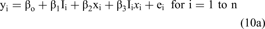
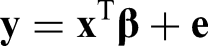
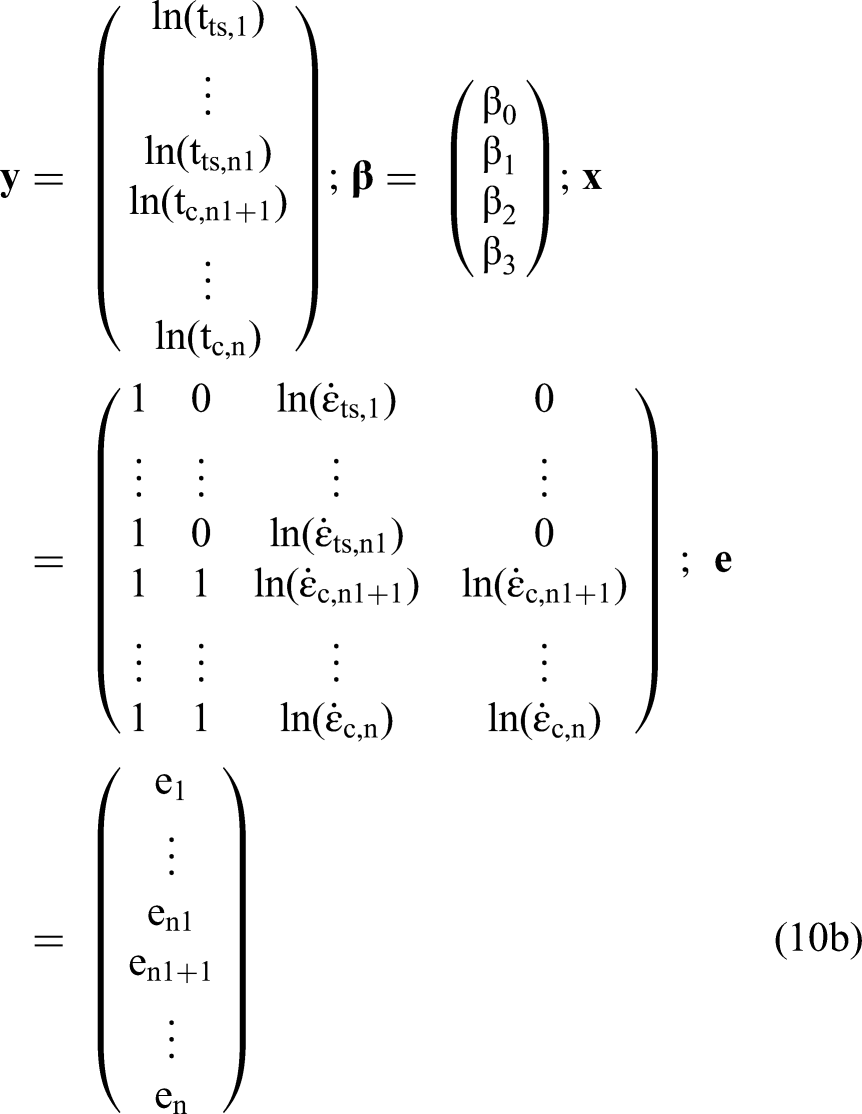
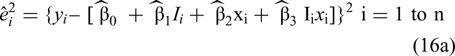
where β₀= ln(M_ts), β₀+ β₁= ln(M_c), β₂= ρ_ts and β₂+ β₃= ρ_c. Consequently, testing the Levi De Oliveira Bueno hypothesis boils down to testing the dual hypothesis that β₁= 0 and β₃= 0. The variable e_i in Eq. (10a) represents the scatter that is measured around the regression line and reflects the stochastic nature of creep and tensile testing. In matrix form, Eq. (10a) can be written as

$$\mathbf{y}={\mathbf{x}}^{\mathrm{T}}\beta +\mathbf{e}$$

where

$$\mathbf{y}=\left(\begin{array}{c}\ln ({\mathrm{t}}_{\mathrm{ts},1})\\ ⋮\\ \ln ({\mathrm{t}}_{\mathrm{ts},\mathrm{n}1})\\ \ln ({\mathrm{t}}_{\mathrm{c},\mathrm{n}1+1})\\ ⋮\\ \ln ({\mathrm{t}}_{\mathrm{c},\mathrm{n}})\end{array}\right);\beta =\left(\begin{array}{c}{\beta }_0\\ {\beta }_1\\ {\beta }_2\\ {\beta }_3\end{array}\right);\mathbf{x}=\left(\begin{array}{cccc}1& 0& \ln ({\dot{\epsilon }}_{\mathrm{ts},1})& 0\\ ⋮& ⋮& ⋮& ⋮\\ 1& 0& \ln ({\dot{\epsilon }}_{\mathrm{ts},\mathrm{n}1})& 0\\ 1& 1& \ln ({\dot{\epsilon }}_{\mathrm{c},\mathrm{n}1+1})& \ln ({\dot{\epsilon }}_{\mathrm{c},\mathrm{n}1+1})\\ ⋮& ⋮& ⋮& ⋮\\ 1& 1& \ln ({\dot{\epsilon }}_{\mathrm{c},\mathrm{n}})& \ln ({\dot{\epsilon }}_{\mathrm{c},\mathrm{n}})\end{array}\right);\mathbf{e}=\left(\begin{array}{c}{\mathrm{e}}_1\\ ⋮\\ {\mathrm{e}}_{\mathrm{n}1}\\ {\mathrm{e}}_{\mathrm{n}1+1}\\ ⋮\\ {\mathrm{e}}_{\mathrm{n}}\end{array}\right)$$

(10\rm b)

The ordinary least squares procedure estimates the parameters β₀ to β₃ as those values which minimise Σe²_i (i = 1 to n). The solution to this least squares problem is

$$\hat{\beta }=({\mathbf{x}}^{\mathrm{T}}\mathbf{x}{)}^{-1}{\mathbf{x}}^{\mathrm{T}}\mathbf{y}$$

(11\rm a)

where $\hat{\beta }$ is the least squares estimator of $\beta$ , x^T is the transpose of x and ()⁻¹ is the inverse of the matrix in the brackets. These least squares estimators are called linear estimators as they are a linear combination of the y_i. They are sample estimates as collecting a different creep and tensile sample of the same sizes will result in different values for ${\hat{\beta }}_o$ to ${\hat{\beta }}_3$ . Next assume that the values for x_i are fixed numbers (or alternatively are uncorrelated with the e_i), and that the mean of all the e_i values equals zero. Then, it can be shown that if all possible samples of size n₁ and n-n₁ of observations on y_i and x_i are taken, and for each sample the estimates ${\hat{\beta }}_{\mathrm{o}}$ to ${\hat{\beta }}_3$ are computed, then a large number of estimates for each will be obtained and the means (called the expected value E) of these values will equal the true (i.e., population) parameter values. For example, E[ ${\hat{\beta }}_o$ ] =  ${\beta }_o$ and E[ ${\hat{\beta }}_3$ ] =  ${\beta }_3$ . So, the least squares estimates are said to be unbiased.

If the residuals e_i from both the creep and tensile data have the same constant variance equal to ${\sigma }_e^2$ , and if the e_i are all independent of each other, then the covariance matrix for $\hat{\beta }$ is given by

$$\mathrm{Var}(\hat{\beta })={\sigma }_e^2({\mathbf{x}}^{\mathrm{\top }}\mathbf{x}{)}^{-1}$$

(11\rm b)

and so Var( $\hat{\beta }$ ) is a 4 × 4 square matrix. The diagonal of this matrix contains the variances of ${\hat{\beta }}_o$ to ${\hat{\beta }}_3$ (for example, Var( ${\hat{\beta }}_o)$ is in position (1,1) of the matrix and Var( ${\hat{\beta }}_3)$ is in position (4,4) of the matrix). The covariances between these parameter estimates are then in the of-diagonal positions. The variance of each least squares estimate - given by Eq. (11b) - also has the smallest variance amongst the class of all possible linear estimators. This in combination with their unbiased nature ensures that the chances of obtaining an estimate for each β that is different from their true values is minimised. It is this result that makes the least squares estimation procedure so popular.

If in addition to the above assumptions, the residuals e_i are assumed to be normally distributed, then the y_i and each ${\hat{\beta }}_j$ variate will also be normally distributed. Each ${\hat{\beta }}_j$ will then have a normal distribution with a mean value equal to their true value and with minimised variances

$${\hat{\beta }}_{\mathrm{j}}\sim \mathrm{N}[{\beta }_{\mathrm{j}},\mathrm{Var}({\hat{\beta }}_{\mathrm{j}})]$$

(12)

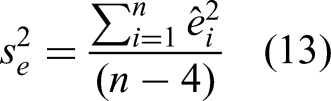
Unfortunately, ${\sigma }_e^2$ is rarely known in Eq. (11b) and needs to be estimated from the sample of data. It can be shown that an unbiased estimate of this residual variance is

$$s_e^2={\displaystyle \frac{{\sum }_{i=1}^n{\hat{e}}_i^2}{(n-4)}}$$

(13)

where the ${\hat{e}}_i^2$ are calculated from Eqs. (10a) using the parameter estimates given by Eq. (11a). If in Eq. (11b), ${\sigma }_e^2$ is replaced with $s_e^2$ , then

$$t^g={\displaystyle \frac{{\hat{\beta }}_j-{\beta }_j}{\sqrt{\mathrm{Var}({\hat{\beta }}_{\mathrm{j}})]}}}$$

(14)

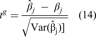
has a student t distribution with n – 4 degrees of freedom. Any hypothesised value for β_j can be tested by simply substituting into Eq. (14) the hypothesised value for β_j. For example, consider the null hypothesis that the MG exponent is the same in the creep and tensile data sets. This can now be tested by expressing the null hypothesis as ${\beta }_3$  = 0. Substituting this value into Eq. (14)

$$t^g={\displaystyle \frac{{\hat{\beta }}_3-0}{\sqrt{Var({\beta }_3)}}}$$

(15)

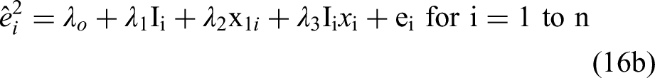
where ${\hat{\beta }}_3$ is located in the 4th row of $\hat{\beta }$ in Eq. (11a) and $\mathrm{Var}({\hat{\beta }}_3)$ is located in position (4,4) of the matrix Var( $\hat{\beta }$ ) in Eq. (11b). If the |t^g| value is less than |t_α/2,n−4| the null hypothesis is accepted. The Levi De Oliveira Bueno hypothesis, at least in part, can now be tested by expressing the null hypothesis as H_o: ${\beta }_3$  = 0. To sum up, the t test of a single parameter restriction requires the following assumptions to hold: i. The e_i are normally distributed, ii the e_i over all n data points (i.e., in the creep and tensile data sets) have the same constant variance (homoscedastic residuals) and iii. the covariance between x_1i and e_i is zero).

White ¹⁹ suggested the following test for homoscedastic residuals. First, estimate values for the squared residuals

$$\begin{array}{r}{\hat{e}}_i^2=\{y_i\text{–}[{\hat{\beta }}_0+{\hat{\beta }}_1{I}_i+{\hat{\beta }}_2{\mathrm{x}}_{\mathrm{i}}+{\hat{\beta }}_3{\mathrm{I}}_{\mathrm{i}}{x}_{\mathrm{i}}]{\}}^2\mathrm{i}=1\mathrm{to}\mathrm{n}\end{array}$$

(16\rm a)

where the ${\hat{\beta }}_{\mathrm{j}}$ and found from Eq. (11a). Then carry out the regression

$$\begin{array}{r}{\hat{e}}_i^2={\lambda }_o+{\lambda }_1{\mathrm{I}}_{\mathrm{i}}+{\lambda }_2{\mathrm{x}}_{1i}+{\lambda }_3{\mathrm{I}}_{\mathrm{i}}{x}_{\mathrm{i}}+{\mathrm{e}}_{\mathrm{i}}\mathrm{for}\mathrm{i}=1\mathrm{to}\mathrm{n}\end{array}$$

(16\rm b)

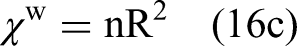
${\hat{e}}_i^2$ is an estimate of the residual variance (as the residuals are assumed to have zero mean) when the log strain rate equals x_i. So constant residual variance requires ${\hat{e}}_i^2$ to be independent of x_1i, i.e_., requires λ₁= λ₂= λ₃= 0. This will only be the case if the R² value associated with Eq. (16b) is close to zero. So, if the null hypothesis of homoscedastic residuals is true, the statistic

$${\chi }^{\mathrm{w}}={\mathrm{nR}}^2$$

(16\rm c)

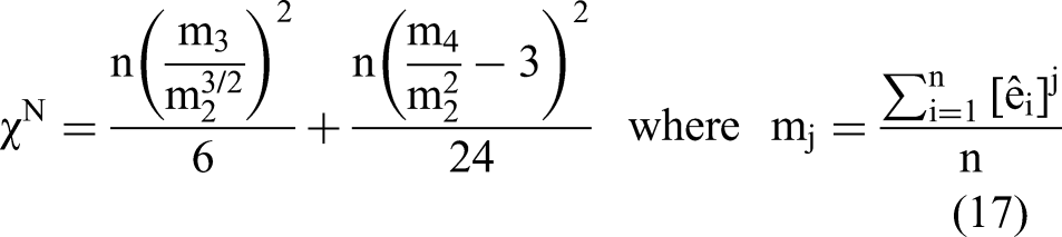
has a chi square distribution with n-1 degrees of freedom. Bowman and Shenton ²⁰ and Jarque and Bera ²¹ proposed the following test for normally distributed variables. It is based on sample measures of Skewness and Kurtosis and is given by

$$\begin{array}{r}{\chi }^{\mathrm{N}}={\displaystyle \frac{\mathrm{n}{\left({\displaystyle \frac{{\mathrm{m}}_3}{{\mathrm{m}}_2^{3/2}}}\right)}^2}{6}+{\displaystyle \frac{\mathrm{n}{\left({\displaystyle \frac{{\mathrm{m}}_4}{{\mathrm{m}}_2^2}-3}\right)}^2}{24}\mathrm{where}{\mathrm{m}}_{\mathrm{j}}={\displaystyle \frac{{\sum }_{\mathrm{i}=1}^{\mathrm{n}}{[{\hat{\mathrm{e}}}_{\mathrm{i}}]}^{\mathrm{j}}}{\mathrm{n}}}}}\end{array}$$

(17)

The first term measures the degree of skewness in the residual distribution which equals zero when the distribution is symmetric. The second term measures the flatness of the distribution that again equals zero when it corresponds to the degree of flatness associated with the normal distribution. Under the null hypothesis of normality, this test statistic should be close to zero and follows a chi distribution with 2 degrees of freedom. So, if the value for ${\chi }^{\mathrm{N}}$ exceeds the selected critical value for χ, the null hypothesis of normality is rejected.

Unfortunately, this test has poor small sample properties and a version of this test with a sample size correction can be found in Doornick and Hansen. ²² This modification has a chi square distribution with 2 degrees of freedom under the null hypothesis - even in small samples.

Testing multiple parameter restrictions when the Monkman-Grant exponent is less than 1

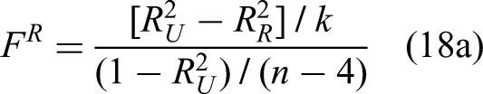
The above t tests can only be used for testing a single parameter restriction, but the Levi De Oliveira Bueno hypothesis involves the two restrictions β₁= β₃= 0 when the MG exponent is not known to equal unity. The F test for such multiple parameter restrictions requires the same assumptions as with the above t tests, and is written as

$$F^R={\displaystyle \frac{[R_U^2-R_R^2]/k}{(1-R_U^2)/(n-4)}}$$

(18\rm a)

where k equals the number of restrictions. $R_U^2$ is the coefficient of determination associated with the unrestricted regression given by Eq. (10a)

$$R_U^2=1-{\displaystyle \frac{{\sum }_{i=1}^n{\hat{e}}_i^2}{{\sum }_{i=1}^n{(y_i-\overline{y})}^2}}$$

(18\rm b)

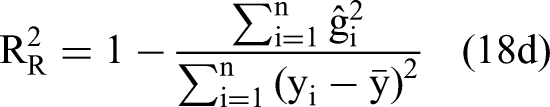
$R_R^2$ is the coefficient of determination associated with the restricted regression (which is determined by the nature of the null hypothesis). For example, to test the Levi De Oliveira Bueno hypothesis, the null hypothesis is β₁= β₃= 0 and so k = 2 within Eq. (18a), and $R_R^2$ is the coefficient of determination associated with the regression under this null hypothesis, which is

$${\mathrm{y}}_{\mathrm{i}}={\beta }_{\mathrm{o}}+{\beta }_2{\mathrm{x}}_{\mathrm{i}}+{\mathrm{g}}_{\mathrm{i}}$$

(18\rm c)

and so

$${\mathrm{R}}_{\mathrm{R}}^2=1-{\displaystyle \frac{{\sum }_{\mathrm{i}=1}^{\mathrm{n}}{\hat{\mathrm{g}}}_{\mathrm{i}}^2}{{\sum }_{\mathrm{i}=1}^{\mathrm{n}}{({\mathrm{y}}_{\mathrm{i}}-\overline{\mathrm{y}})}^2}}$$

(18\rm d)

where ${\hat{g}}_i^2$ are calculated from Eqs. (18c) using the least squares estimates of the parameters β₀ and β₂. A well-known statistical theorem states that the square of a standard normal variate has a chi square distribution with 1 degree of freedom and the square of two standard normal variates has a chi square distribution with 2 degrees of freedom and so on. Further, the ratio of two chi square variables has an F distribution. So, if the residuals e_i and g_i are normally distributed, then given Eq. (18b), R²_U involves the sum of n squared normal variates and so irrespective of the null hypothesis, the variable in the denominator of F^R has a chi square distribution with n - 4 degrees of freedom (4 degrees of freedom are lost from n in estimating 4 parameters). The numerator of F^R also has a chi square distribution but only if the null hypothesis is true - with the degrees of freedom equal to the number of restrictions under the null hypothesis (if the null hypothesis is not true the numerator has a non-central chi square distribution as it will then involve the sum of the squared residuals whose mean is not zero).

If, and only if, the null hypothesis is true, F^R will have an F distribution with k and n – 4 degrees of freedom. Consequently, if the value for F^R in Eq. (18a) exceeds F_α, then the observed value for F^R has less than a α% chance of being observed. The fact that it is observed can only then be explained by F^R not having an F distribution – which will only be so if the null hypothesis is not true. Here F_α is the value for F^R such that there is only a probability of α that this value or more will be observed. So, the null hypothesis is rejected only if F^R> F_α, i.e., when the chances of the null hypothesis being true have dropped so low that it cannot be entertained as a realistic possibility.

At a more intuitive level, if the null hypothesis is true, allowing the values for β₀ and β₂ to be different values in the tensile data compared to the creep data, should not explain any more of the variation in all the observed failure times. That is, under the null hypothesis $R_U^2-R_R^2\cong 0$ and F^R in Eq. (18a) will be small in magnitude. The larger it is, the more likely it is therefore that the null hypothesis is false and when its value exceeds F_α, the chances of the null hypothesis being true is at least as as low as α%. Given this low probability, the null hypothesis would then be rejected.

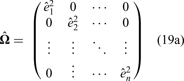
These F tests are uniformly most powerful tests for parameter restrictions under the above three assumptions. The reason for requiring homoscedastic residuals is that if the residual variance is larger in the tensile data set, it will deflate the value for $R_U^2$ and so inflate the value for F^R even if the null hypothesis is true. These so-called heteroscedastic residuals will therefore tend to lead to researchers rejecting the null hypothesis even when it is true. The heteroscedasticity problem can be overcome by adjusting the standard errors of the parameter estimates in Eqs. (11b) to adjust for this heteroscedasticity. As discussed above, White ¹⁹ suggested the variance in e_i associated with each value of x_i can be estimated using the estimated squared residuals. If the estimated squared residuals calculated using Eq. (16b) are placed down the diagonal of square matrix $\mathbf{\Omega }$

$$\hat{\mathbf{\Omega }}=\left(\begin{array}{cccc}{\hat{e}}_1^2& 0& \cdots & 0\\ 0& {\hat{e}}_2^2& \cdots & 0\\ ⋮& ⋮& \ddots & ⋮\\ 0& ⋮& \cdots & {\hat{e}}_n^2\end{array}\right)$$

(19\rm a)

then White showed that the standard errors for the parameters ${\hat{\beta }}_{\mathrm{j}}$ in Eq. (11a), corrected for any heteroscedasticity in the residuals, is given by

$$\mathrm{Var}(\hat{\beta })={\displaystyle \frac{\mathrm{n}}{n-4}({\mathbf{x}}^{\mathit{T}}\mathbf{x}{)}^{-1}({\mathbf{x}}^{\mathrm{T}}\hat{\mathbf{\Omega }}\mathbf{x})({\mathbf{x}}^{\mathit{T}}\mathbf{x}{)}^{-1}}$$

(19\rm b)

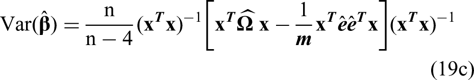
The square root of the values on the diagonal of this matrix are often termed heteroscedastic consistent standard errors, or HCSE for short. Appendix C shows that Eq. (19b) is a consistent or asymptotic estimator of Var( $\hat{\beta }$ ), which implies that the estimator is valid, strictly speaking, only for very large data sets. MacKinnon and White ²³ showed that in small samples Eq. (19c) produced a better estimate of the true variance for Var( $\hat{\beta }$ ) (see Appendix C)

$$\mathrm{Var}(\hat{\beta })={\displaystyle \frac{\mathrm{n}}{\mathrm{n}-4}({\mathbf{x}}^{\mathit{T}}\mathbf{x}{)}^{-1}\left[{\mathbf{x}}^{\mathit{T}}\hat{\mathbf{\Omega }}\mathbf{x}-{\displaystyle \frac{1}{\mathit{m}}{\mathbf{x}}^{\mathit{T}}\hat{\mathit{e}}{\hat{\mathit{e}}}^{\mathit{T}}\mathbf{x}}\right]({\mathbf{x}}^{\mathit{T}}\mathbf{x}{)}^{-1}}$$

(19\rm c)

where $\hat{\mathit{e}}$ is a vector of the ${\hat{e}}_i^2$ . White and MacKinnon ²³ showed that in small samples Eq. (19c) produced a better estimate of the true variance for Var( $\hat{\beta }$ ). The square root of the values on the diagonal of this matrix are often termed Jackknife heteroscedastic consistent standard errors, or JHCSE for short. The test statistic t^g can now be corrected for any heteroscedasticity by simply using Eq. (19c) for the denominator in Eq. (14).

Multiple constraints corrected for any heteroscedasticity can now be tested for by writing multiple constraints in matrix form

$$\mathbf{p}=\mathbf{R}\hat{\beta }=\mathbf{q}$$

(20\rm a)

where vector $\hat{\beta }$ is a sample estimate of β and each row of R corresponds to a single parameter constraint and q contains the constrained parameter value. For example, Levi De Oliveira Bueno informally looked at whether β₃= 0, when the restrictions β₁= -1 is assumed true. This dual set of restrictions can be written as

$$\mathbf{R}=\left(\begin{array}{cccc}0& 1& 0& 0\\ 0& 0& 0& 1\end{array}\right)\mathrm{and}\mathbf{q}=\left(\begin{array}{c}-1\\ 0\end{array}\right)$$

(20\rm b)

Appendix C demonstrates that the matrix p will follow a normal distribution provided $\hat{\beta }$ is normally distributed (as it is a linear combination of them) which in turn requires the residuals to be normally distributed with a mean vector of zero. Given that $\hat{\beta }$ is unbiased, the mean value for p is zero

$$\mathbf{p}\sim N[\mathbf{0},Var(\mathbf{p})]$$

with the covariance matrix of p given by

$$Var(\mathbf{p})=\mathbf{R}Var[\hat{\beta }]{\mathbf{R}}^T$$

(21\rm a)

Var[ $\hat{\beta }$ ] is given by Eq. (19b) for the asymptotic test or Eq. (19c) for the finite sample version of this test. So if the null hypotheses H₀: $R\mathit{\beta }=\mathit{q}$ is true, the Wald statistic

$${\mathrm{W}}_{\mathrm{k}}={\mathbf{p}}^{\mathrm{T}}[Var(\mathbf{p}){]}^{-1}\mathbf{p}$$

(21\rm b)

has a chi square distribution with k degrees of freedom. k corresponds to the number of constraints being tested and so equals the number of rows contained in R and q. This is because the square of a standard normal variate has a chi squares distribution (with k degrees of freedom as p is a kx1 vector containing k standardised variates). There are two versions of this test. $W_k^W$ is the value for W_k in Eq. (21b) when $V\mathrm{ar}(\hat{\beta })$ is given by Eq. (19b), whilst $W_k^{JK}$ is the value for W_k in Eq. (21b) when $V\mathrm{ar}(\hat{\beta })$ is given by Eq. (19c). In either case it is a test for multiple restrictions adjusted for any heteroscedasticity in the residuals and so is more flexible than the F^R test in Eq. (18a) as that is invalid for non-constant variance in the residuals. An F variant of this test is found by dividing through by the number of restrictions being tests. If the null hypothesis is true, $F^W=\frac{W_k^W}{k}$ and $F^{JK}=\frac{W_k^{JK}}{k}$ follow a F distributions with k and n-4 degrees of freedom.

Predictions

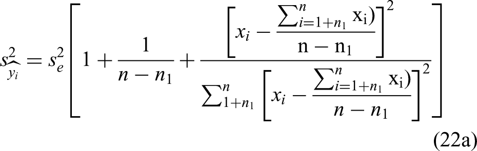
Another approach to assessing the Levi De Oliveira Bueno hypothesis is to estimate the MG relation using just the tensile test data. If the hypothesis is true, then the resulting estimated relation should produce unbiased forecasts of the failure times associated with the creep data set and the actual creep failure times should then be within a multiple of the variability of the predictions given by

$$s_{\widehat{y_i}}^2=s_e^2\left[1+{\displaystyle \frac{1}{n-n_1}+{\displaystyle \frac{{\left[x_i-{\displaystyle \frac{{\sum }_{i=1+n_1}^n{\mathrm{x}}_{\mathrm{i}})}{\mathrm{n}-{\mathrm{n}}_1}}\right]}^2}{{\sum }_{1+n_1}^n{\left[x_i-{\displaystyle \frac{{\sum }_{i=1+n_1}^n{\mathrm{x}}_{\mathrm{i}})}{n-n_1}}\right]}^2}}}\right]$$

(22\rm a)

Eq. (22a) picks up variability due to the residuals e_i and uncertainty about the parameter estimates. An approximate 95% confidence interval for any prediction of y_i is then given by

$${\hat{y}}_i=({\hat{\beta }}_0+{\hat{\beta }}_2{x}_{1i})\mp 2(s_{\widehat{y_i}})$$

(22\rm b)

where ${\hat{\beta }}_0,{\hat{\beta }}_2$ are estimated from

$${\mathrm{y}}_{\mathrm{i}}={\beta }_{\mathrm{o}}+{\beta }_2{\mathrm{x}}_{\mathrm{i}}+{\mathrm{e}}_{\mathrm{i}}\mathrm{for}\mathrm{i}=1\mathrm{to}{\mathrm{n}}_1$$

using only the tensile data

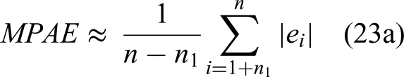
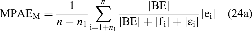
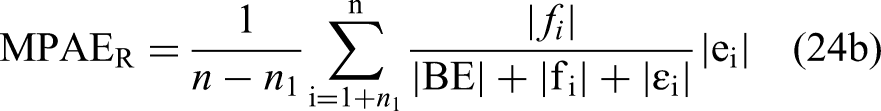
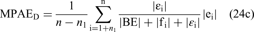
Evans ²⁴ suggested the randomness of the prediction errors is best measured using the mean percentage absolute error (MPAE). Following Robeson and Cort, ²⁵ the MPAE is formally defined as

$$MPAE\approx {\displaystyle \frac{1}{n-n_1}\sum _{i=1+n_1}^n|e_i|}$$

(23\rm a)

where e_i is the difference between the actual log time to failure at creep test condition i and the corresponding log time to failure predicted by the MG relation estimated from the tensile data set. As this prediction error is expressed in terms of (natural) log differences, this represents an approximate percentage error. Robeson and Cort showed that the MPAE can be decomposed into three separate parts. The first component of |e_i| is the absolute bias error $|BE|=|(\overline{y_i}-\overline{{\hat{y}}_i})$ |, where the bar indicates the average values for the actual and predicted value for y). Robeson and Cort then remove this component by adding it onto the predictions, ${\hat{y}}_{pi}={\hat{y}}_i$ + $|BE|$ . |BE| is clearly a systematic prediction error. They then use least squares to determine the values for δ₀ and δ₁ in the regression

$${\mathrm{y}}_{\mathrm{i}}={\delta }_0+{\delta }_1{\hat{\mathrm{y}}}_{pi}+{\epsilon }_{\mathrm{i}}$$

(23\rm b)

The second part is also a systematic prediction error and is equal to |f_i| = | ${\hat{y}}_{pi}-($ δ₀+ δ₁ ${\hat{y}}_{pi})$ |. This quantity only exists if δ₁ is different from 1 and δ₀ is different from 0. Robeson and Willmott call this component the proportionality error. The third component is a random prediction error and equals |ε_i|. On this basis, the decomposition of the MPAE is

$${\mathrm{MPAE}}_{\mathrm{M}}={\displaystyle \frac{1}{n-n_1}\sum _{\mathrm{i}=1+n_1}^n{\displaystyle \frac{|\mathrm{BE}|}{|\mathrm{BE}|+|{\mathrm{f}}_{\mathrm{i}}|+|{\epsilon }_{\mathrm{i}}|}|{\mathrm{e}}_{\mathrm{i}}|}}$$

(24\rm a)

$${\mathrm{MPAE}}_{\mathrm{R}}={\displaystyle \frac{1}{n-n_1}\sum _{\mathrm{i}=1+n_1}^{\mathrm{n}}{\displaystyle \frac{|f_i|}{|\mathrm{BE}|+|{\mathrm{f}}_{\mathrm{i}}|+|{\epsilon }_{\mathrm{i}}|}|{\mathrm{e}}_{\mathrm{i}}|}}$$

(24\rm b)

$${\mathrm{MPAE}}_{\mathrm{D}}={\displaystyle \frac{1}{n-n_1}\sum _{\mathrm{i}=1+n_1}^{\mathrm{n}}{\displaystyle \frac{|{\epsilon }_{\mathrm{i}}|}{|\mathrm{BE}|+|{\mathrm{f}}_{\mathrm{i}}|+|{\epsilon }_{\mathrm{i}}|}|{\mathrm{e}}_{\mathrm{i}}|}}$$

(24\rm c)

These can be expressed as proportions of MPAE

$$|U_M|={\mathrm{MPAE}}_{\mathrm{M}}/\mathrm{MPAE};|U_R|={\mathrm{MPAE}}_{\mathrm{R}}/\mathrm{MPAE};|U_D|={\mathrm{MPAE}}_{\mathrm{D}}/\mathrm{MPAE}$$

(24\rm d)

If the Levi De Oliveira Bueno hypothesis is true, the expectation is that $|U_D|\approx$ 1 or 100%, so that the MG relation in the tensile test data predicts creep failure times with an average error of zero - as the 0= MPAE_M= MPAE_R.

Results

What Levi De Oliveira Bueno found

Levi De Oliveira Bueno assessed their hypothesis by fitting the MG relation to the creep data set and seeing how well it extrapolated to the lower times (to UTS) associated with the tensile test data assuming ${\rho }_c$  = 1 in Eq. (1b). Using the digitised data from the paper by Levi De Oliveira Bueno, ln(M_c) was estimated as

$${\overline{\mathrm{w}}}_{\mathrm{c}}=-3.0025$$

Consequently, the estimate for M_c was found to be exp(−3.0025) = 0.050. This is very close the value reported by Levi De Oliveira Bueno ¹⁰ in Figure 2(a) in Ref [10], namely, 0.051. This small difference is most likely due to digitising the results from that paper.

Figure 2.

Extrapolation of the MG relation fitted to the tensile test data when forcing ρ_ts= 1.

The solid line in Figure 2 plots ${\mathrm{t}}_{\mathrm{cf}}=0.05({\dot{\epsilon }}_{\mathrm{mc}}{)}^{-1}$ and the dashed line is the extrapolation of this relation to the tensile test results. The extrapolation to the tensile test data in Figure 2 looks reasonable and Levi De Oliveira Bueno stated “The agreement of the CSR tensile data with the creep results, according to the Monkman-Grant fit is evident. Therefore, the scatter observed on the creep data in this kind of plots could be of the same nature as observed for the CSR results”. In this quote, CSR refers to the tensile test data.

Figure 3.

(a) Variation of the minimum creep rate with the rupture time in creep test data, plotted together with the strain rate and time to occurrence of the ultimate tensile stress in the constant strain rate tensile tests. Straight lines refer to the least squares estimates of the MG relation in the creep data (solid line) with extrapolation to the tensile data (dashed line). (b) Creep failure time predictions given by the dashed line in (a) are plotted against the actual creep failure times.

This paper expands on this analysis by considering the following questions:

Does the extrapolation work in the opposite direction?

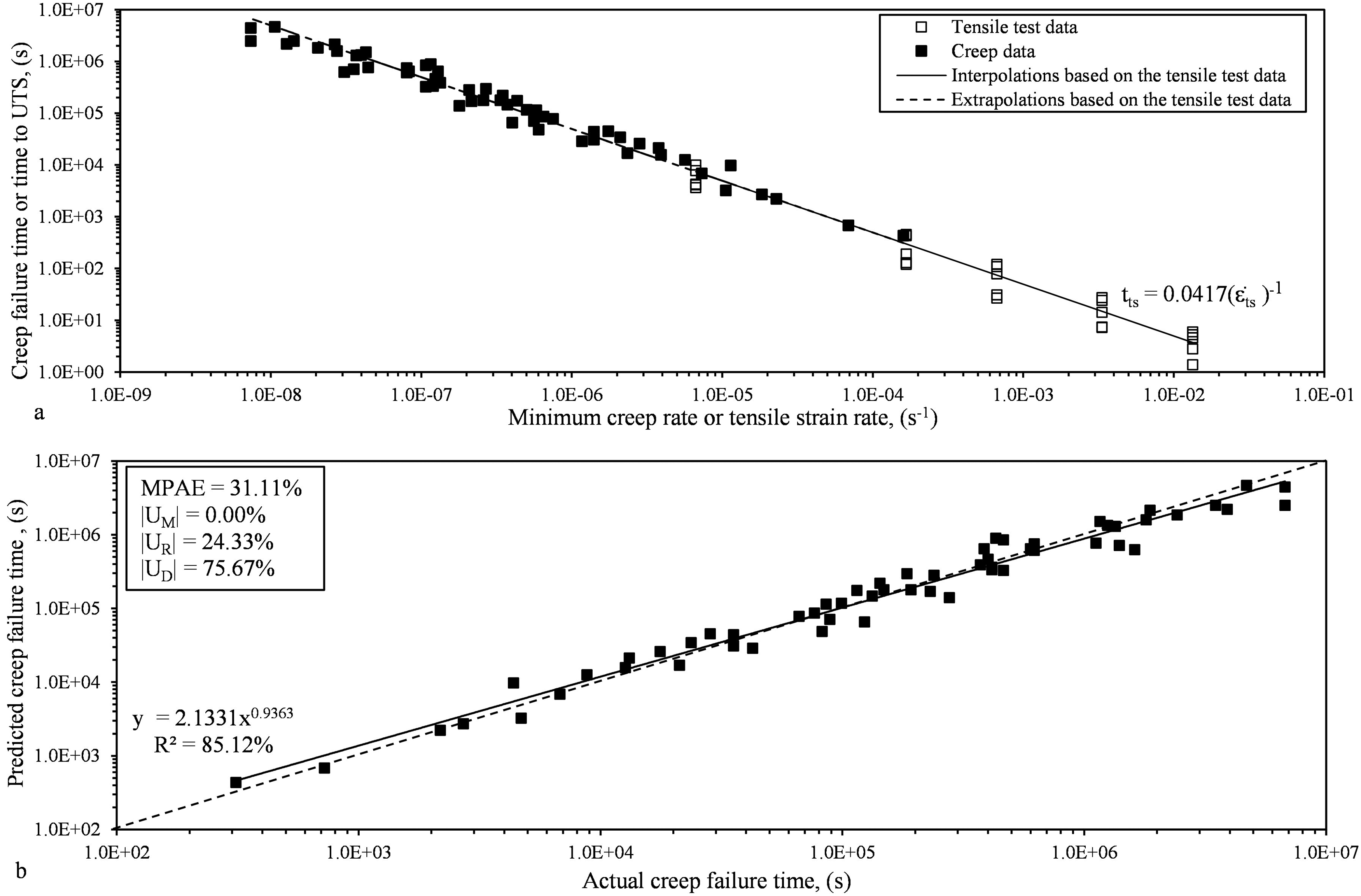
Given the benefit of the Levi De Oliveira Bueno hypothesis being valid, is to predict creep failure times associated with typical operating conditions from the very short test times associated with tensile data, it seems reasonable to fit the MG relation to the tensile data and see how well it extrapolates to the creep failure times, assuming ρ_ts= 1. The results are shown in Figures 3. Using the digitised data from the paper by Levi De Oliveira Bueno, and based on Eq. (4a), ln(M_ts) is estimated as

$${\overline{\mathrm{w}}}_{\mathrm{ts}}=-3.1773$$

Consequently, the estimate for M_ts was found to be exp(−3.1773) = 0.0417. The solid line in Figure (3a) plots ${\mathrm{t}}_{\mathrm{ts}}=0.0417({\dot{\epsilon }}_{\mathrm{ts}}{)}^{-1}$ with the dashed segment of this line showing the extrapolation of this relationship to the creep failure times. The predicted creep failure times along this extrapolated lines look very good. This is confirmed in Fig. (3b) where these creep failure time predictions are plotted against the actual creep failure times. The MPAE in the creep failure time predictions is some 31.11%. The best fit line to the data points in this figure is slightly flatter the ideal 45° line – given by the dashed line in Figure (3b). 24.33% of the MPAE is explained by this phenomenon (=|U_D|). The remaining part of the MPAE is random in nature – some 75.67% (=|U_R|).

Despite the reasonable fit shown in Figures (3), are the MG constants M_c and M_ts really equal if ρ_c= ρ_ts= 1?

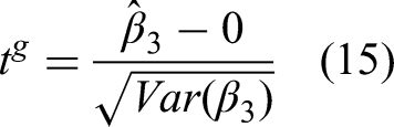
As can be seen from Figure 3 and Figure 2, the values for M_c and M_ts are quite different, and despite this, the predictions made from the tensile test data are quite good. So, are these differences statistically significant? When ρ_c= ρ_ts= 1, then in Eq. (10a) β₂= −1 and β₃= 0 giving

$${\mathrm{y}}_{\mathrm{i}}+{\mathrm{x}}_{1\mathrm{i}}={\beta }_{\mathrm{o}}+{\beta }_1{\mathrm{I}}_{\mathrm{i}}+{\mathrm{v}}_{\mathrm{i}}\mathrm{for}\mathrm{i}=1\mathrm{to}\mathrm{n}$$

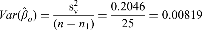
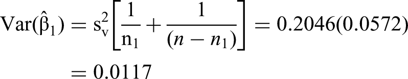
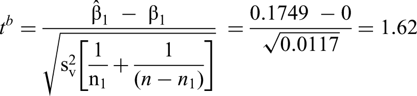
where the n = 83 observations are from the creep and tensile data sets combined. Here β₀= ln(M_ts) and β₀+ β₁= ln(M_c). So, given the assumption that ρ_c= ρ_ts= 1, M_c= M_ts, only when β₁= 0. Estimated values for M_c and M_ts where given in the previous sub section, giving the estimates ${\hat{\beta }}_0={\overline{\mathrm{w}}}_{\mathrm{ts}}$ and ${\hat{\beta }}_1$ = ${\overline{\mathrm{w}}}_{\mathrm{c}}-$ ${\overline{\mathrm{w}}}_{\mathrm{ts}}$ (see Eq. (7b)). So for this sample of data, ln(M_c) exceeds ln(M_ts) by 0.1749. From Eq.(8b), s²_v was found to be 0.2046, which is equal to the pooled variance s²_w in Eq. (A3). Then from Eq. (B1)

$$Var({\hat{\beta }}_o)={\displaystyle \frac{{\mathrm{s}}_{\mathrm{v}}^2}{(n-n_1)}={\displaystyle \frac{0.2046}{25}=0.00819}}$$

$$\mathrm{Var}({\hat{\beta }}_1)={\mathrm{s}}_{\mathrm{v}}^2\left[{\displaystyle \frac{1}{{\mathrm{n}}_1}+{\displaystyle \frac{1}{(n-n_1)}}}\right]=0.2046(0.0572)=0.0117$$

The null hypothesis that β₁= 0 can be tested using the t statistic of Eq. (8a)

$$t^b={\displaystyle \frac{{\hat{\beta }}_1-{\beta }_1}{\sqrt{{\mathrm{s}}_{\mathrm{v}}^2\left[{\displaystyle \frac{1}{{\mathrm{n}}_1}+{\displaystyle \frac{1}{(n-n_1)}}}\right]}}={\displaystyle \frac{0.1749-0}{\sqrt{0.0117}}=1.62}}$$

At the 5% significance level the critical value for t is |t_α/2,n−2| = |t_{0.05/2,83−2}| = 1.99 and so the null hypothesis of β₁= 0 is accepted. Put differently, the p-value of 0.11 suggests that the probability of the null hypothesis being true is 11% which is too high to be able to reject the null hypothesis (with a 5% significance level, the chances of wrongly rejecting the null hypothesis must be lower than 5%). This test suggests that if ρ_c= ρ_ts= 1, the Monkman Grant relation is the same in the creep and tensile data sets, i.e., under this condition the Levi De Oliveira Bueno cannot be rejected with the required degree of confidence. This supports the conclusion drawn in the previous sub section. But how reliable is this test?

First it requires the v_i to have constant variance or equivalently for σ²_wc= σ²_wts= σ²_w. Using Eq. (A2), the F^V test of Eq. (6) comes out at

$${\mathrm{F}}^{\mathrm{V}}={\displaystyle \frac{S_{{\mathrm{w}}_{ts}}^2}{S_{{\mathrm{w}}_c}^2}={\displaystyle \frac{0.3214}{0.1555}=2.07}}$$

At the 5% significance level, the critical value for F^V is |F_α,n1,n−n1| = |t_0.05,24,57| = 1.71. and so the null hypothesis σ²_wc= σ²_wts is rejected at this significance level, i.e., can be rejected with less that a 5% chance of being wrong. But at the 1% significance level the critical value for F^V= 2.13 and so only at this lower significance level can the null hypothesis of σ²_wc= σ²_wts be accepted. Given this, it seems sensible to use the HCSE (of Eq. (19c) in the t^b test

$$t^b={\displaystyle \frac{{\hat{\beta }}_1-{\beta }_1}{\sqrt{\mathrm{Var}({\hat{\beta }}_1)}}={\displaystyle \frac{0.1749-0}{\sqrt{0.0159}}=1.39}}$$

Irrespective of whether there is any heteroscedasticity, the p-value now increases to 0.17 which suggests that the probability of the null hypothesis being true is 17% which is too high to be able to reject the null hypothesis. So provided the v_i are normally distributed, this test is valid. The normality test given by Eq. (17) comes out at ${\chi }^{\mathrm{N}}=4.56$ . At the 5% significance level, normality requires this value to be less than 5.99, and so the assumption of normality of the v_i is accepted at this significance level. With a p-value of 0.102 it is also accepted at the 10% significance level.

Taken all together, the fact that the (heteroscedastic robust) p-value is well above the 10% significance level and that the normality of v_i cannot be rejected at this significance level – the hypothesis that the population values for ln(M_ts) and ln(M_c) are the same, cannot be rejected. The MG constants are not statistically significantly different in value from each other. This is consistent with the good creep failure time predictions made from extrapolating the short time tensile test results.

Are the Monkman-Grant exponents ρ_c and ρ_ts in Eqs. (1b,1e) really equal to 1?

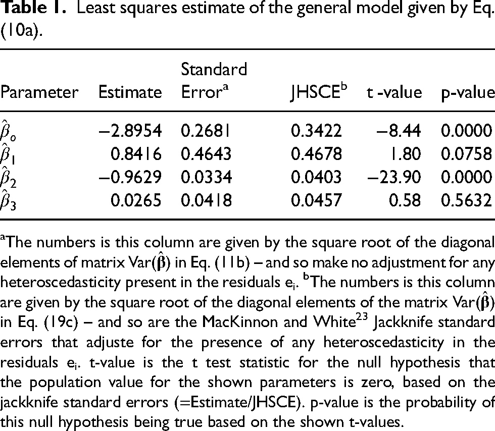
The analysis in the previous sub section, is conditional on ρ_c= ρ_ts= 1 being true. So, this subsection delves into whether this assumption is even true. To test the restriction imposed on the data by Levi De Oliveira Bueno, this restriction is relaxed by using the general model given by Eq.(10a). Table 1 shows the results from estimating the parameters of this model.

Table 1.

Least squares estimate of the general model given by Eq. (10a).

Parameter	Estimate	Standard Errora	JHSCEb	t -value	p-value
${\hat{\beta }}_o$	−2.8954	0.2681	0.3422	−8.44	0.0000
${\hat{\beta }}_1$	0.8416	0.4643	0.4678	1.80	0.0758
${\hat{\beta }}_2$	−0.9629	0.0334	0.0403	−23.90	0.0000
${\hat{\beta }}_3$	0.0265	0.0418	0.0457	0.58	0.5632

^aThe numbers is this column are given by the square root of the diagonal elements of matrix Var( $\hat{\beta }$ ) in Eq. (11b) – and so make no adjustment for any heteroscedasticity present in the residuals e_i. ^bThe numbers is this column are given by the square root of the diagonal elements of the matrix Var( $\hat{\beta }$ ) in Eq. (19c) – and so are the MacKinnon and White ²³ Jackknife standard errors that adjuste for the presence of any heteroscedasticity in the residuals e_i. t-value is the t test statistic for the null hypothesis that the population value for the shown parameters is zero, based on the jackknife standard errors (=Estimate/JHSCE). p-value is the probability of this null hypothesis being true based on the shown t-values.

For ρ_c= ρ_ts= 1 the parameter β₂ must equal −1 (which makes ρ_ts= 1) and the parameter β₃ must equal 0 (which makes ρ_c equal to ρ_ts, which in turn equals 1 when β₂= −1). The t-value for the null hypothesis H_o: β₃= 0 is 0.58 from Table 1, giving a probability that this null hypothesis is true of 56.32%. Thus, this hypothesis easily accepted at the 5% significance level, implying that the Monkman-Grant exponent is the same in the tensile and creep data sets. The t-value for testing the null hypothesis H_o: β₂= −1 is 0.92 (−0.9629– −1)/0.0403 so the probability of this constraint being true is 36%. Again, this hypothesis on its own can be easily accepted, i.e., that that ρ_c= ρ_ts= 1. But can they both be accepted jointly? Well, one thing to note in Table 1, is the parameter standard errors adjusted for heteroscedasticity (column 4) are quite different from the unadjusted standard errors (column 3). Given this, the assumption of constant variance in the e_i looks unlikely to be true and so there is little point in forming the $F^R$ test of Eq. (18a) for this joint restriction as it requires this assumption to be true. So, the Wald test given by Eq. (D11b, D12) that adjusts for heteroscedasticity in the errors is used and comes out as $F_2^{JK}$  = 4.81 with a p-value of 0.011. The chances of ρ_c= ρ_ts and of ρ_c= ρ_ts= 1 being true, is only 1.1%. This hypothesis is clearly rejected at the 5% significance level. The normality of the e_i required for this test to be valid is accepted at the 5% significance level as ${\chi }^{\mathrm{N}}=4.13$ (with a 5% critical value of 5.99). The best conclusion to draw from these results is that the Monkman-Grant exponent has the same value in the creep and tensile data sets, but that this value is less than 1. Consequently, the result shown above that M_c= M_ts, cannot be accepted as a valid result as it was conditional on ρ_c= ρ_ts= 1 being true.

Is the dual constraint (M_c =M_ts and ρ_c= ρ_ts) needed for the Levi De Oliveira Bueno hypothesis to be true accepted by the data?

The equivalence of M_c and M_ts therefore needs to be looked at again with a test that is not conditional on ρ_c= ρ_ts= 1 being true. For the the Levi De Oliveira Bueno hypothesis to be true now requires that M_c= M_ts, (or β₁= 0) and ρ_c= ρ_ts (or β₃= 0). The Wald statistic for testing this joint restriction comes out at $F_2^{JK}$  = 5.72 with a p-value of 0.005. So the chances of ρ_c= ρ_ts and M_c =M_ts being true is only 0.5% and so this hypothesis is clearly rejected even at the 1% significance level. This suggests that the creep failure times predicted from an extrapolation of the MG relation estimated from just the tensile data will consistently over estimate the actual creep failure times as ln(M_c) > (M_ts) by 0.8416 when allowing for the MG exponent to differ from −1.

How random are the errors made in predicting of creep failure times using only tensile test results?

The section looks at whether such predictions are indeed biased. The solid line in Figure 4(a), shows a fit of Eq. (1e) to the tensile test data. This long-dashed line then extrapolates this relation to the creep data set. The resulting creep failure time predictions are towards the lower end of the range of actual creep failure times, suggesting a degree of average bias. The short dashed lines show the approximate 95% confidence interval for these predictions based on Eq. (22a). Whilst all the data points are within these limits, the limits are quite wide and the actual creep failure times tend to cluster more towards the upper rather than the lower limit.

Figure 4.

(a) Extrapolation of the MG relation fitted to the tensile test data allowing ρ_ts< 1. (b) Actual v predicted creep failure times.

In Figure 4(b) the MPAE is almost 50% and is some 20 percentage points higher than when the ρ_ts= 1 constraint is imposed on the tensile data set. What's more, only a third of this MPAE is random in nature – down from 75% when the ρ_ts= 1 constraint is imposed on the tensile data set. As a result, the average prediction error is 61%, whereas as when the ρ_ts= 1 constraint is imposed on the tensile data set, this average error did not exist. So, whilst the ρ_ts= 1 constraint is not the best representation of the tensile data, it produces substantially better creep failure time predictions. The problem is that if tensile data is to be used to predict unknown creep failure times at operating conditions, these times will not be known to assess whether imposing ρ_ts= 1 will produce sensible operating lives.

Conclusion

The Levi De Oliveira Bueno hypothesis offers the possibility of reducing the cost and length of the development cycle for new materials operating at high temperatures. This paper outlined a number of statistical tests for this hypothesis, highlighting clearly the assumptions behind these tests, together with tests for these assumptions being true. Whilst it was found that the MG relation fitted to tensile test data could provide very accurate long term creep life predictions when this exponent of this relation was forced to equal 1, this additional constraint was not accepted by the data using the tests outlines in this paper. When the constraint on this exponent was relaxed, the MG relation fitted to tensile test data was no longer able to predict creep life without bias, with the mean absolute percentage error rising from around 30% to nearly 50%. In fact, the average prediction error made up over 60% of the mean percentage absolute error in predicting creep failure times.

One area of future work would include the application of the statistical tests outlined in this paper to other materials to assess whether the findings of this paper are material specific or apply everywhere. Of particular interest would be an analysis of more ductile materials such as Nickel based super alloys where the value for ρ_c is considerably different from −1 (and so the kinds of equivalence seen in this paper are less likely to holds). In doing this, some consideration should be given to the nature of the tensile testing. It should include testing up to the high strain rates that result in the tensile strength becoming independent of further increases in the strain rate. In addition to this, tests should be carried out down to a temperature where the tensile strain becomes strain invariant. Finally, the sample size should be selected so as to achieve a confidence interval of the required size - n ≈ $(1.96s_e^{/}E{)}^2$ , where E is the required width of the 95% confidence interval for failure time predictions.

Whilst there is quite a lot of creep data in the public domain on such ductile materials (for example, the NIMS creep data bases), assessing the reliability of extrapolating from tensile test data would require additional tensile testing that takes into account the above considerations on the test matrix. If it can be demonstrated that such extrapolations produce creep life predictions with a MPAE whose decomposition has small values for U_M and U_R then this could provide the confidence in the technique required for designers to adopt the approach to developing new materials. A theoretical basis for the equivalence between creep and tensile test data would also help in this respect – indeed this would constitute an important area of future research. A good starting point would be within the theta creep methodology where Evans ²⁶ derived the shape of a uniaxial creep curve in terms on hardening, softening and damage mechanisms. Recently, Harrison et al. ²⁷ showed that this approach to accounting for preexisting damage can explain the shape of a uniaxial creep curve obtained when the stress is varied during a uniaxial creep test. Given that a tensile test can be viewed as a creep test in which the stress is continually changed (to maintain a constant strain rate), this evidence suggests some sort of equivalence between a creep and a tensile test.