
Abstract
I challenge Strong’s findings that student employment is not related to attendance. I argue that the original analysis is guilty of controlling for a post-treatment variable. As a result, the coefficients in the regression model do not show how employment causes changes in attendance. I show that employment likely has a negative effect on attendance even given severe confounding. Academics should, if asked, tell students that their attendance will likely suffer the more paid work they do.
Keywords
Introduction
All of us face competing demands on our time. The same is true of university students. Some of these competing demands come from freely chosen activities: some students may be less able to spend time on the study because they are spending more time on varsity volleyball or on amateur dramatics. Other competing demands spring from necessity: some students may be less able to spend time studying because they are working for money or caring for a dependent family member. Paid employment is a particularly important external commitment. Between 70% and 80% of full-time students work while studying (Dennis et al., 2018; Warrell, 2015). 1 Given this, it is important to know whether paid work has positive or negative effects on how well students do at university. This can be done by focusing on attainment, or grades, or by examining intermediate outcomes which are known to be closely related to attainment, like attendance.
James Strong’s article ‘Identifying and understanding the drivers of student engagement in a school of politics and international relations’, published in this journal earlier this year (Strong, 2022), examines the relationship between employment and attendance as part of a broader study of engagement and attainment involving both quantitative and qualitative data from undergraduate students at Queen Mary, University of London (QMUL). He concluded that there was no significant negative effect of student employment on attendance, and that (conditional on attendance) there was a significant positive association between student employment and attainment. The implication of this finding was that ‘the issue is not so much the absolute amount of time . . . [commitments like paid employment] require, but the fact they sometimes clash with taught classes’, and that departments could therefore improve attendance and thereby attainment by working with students to reduce clashes.
This result was described as counter-intuitive since staff at Queen Mary held the belief that time spent in paid employment was time which was not available for study (p. 7). This belief is entirely reasonable, and indeed is supported by most of the literature on part-time employment and student attainment. Broadly, most studies show a negative link between part-time employment and attainment. 2 Callender (2007), in a study of 1000 students at six UK universities, finds that ‘students working the average number of hours a week (15 hours) were a third less likely to get a good degree than an identical non-working student’, where ‘good degree’ means a degree classification of 2/1 or a 1st. On the specific issue of attendance, Oldfield et al. (2018) find that among undergraduate psychology students an extra hour of paid work per week is associated with a 0.2 percentage point drop in attendance. While part-time work might boost students’ earnings in the future (Geel and Backes-Gellner, 2012), the literature suggests it compromises students’ attainment in the here and now.
In this reply, I argue that Strong’s findings about the link between employment and attendance are comforting but wrong. Specifically, these findings are wrong because the regression models which support the finding include a post-treatment variable, or a variable which comes after the thing supposed to explain the outcome (Angrist and Pischke, 2009: s. 3.2.3; Montgomery et al., 2018). When we remove this post-treatment variable, the negative effects of paid employment on attendance are easily seen. Although there might be some factors associated both with paid employment and attendance, these factors would have to have very large effects to turn the link between paid employment and attendance positive.
What Strong (2022) finds
In the first part of his article, Strong models the attendance and mark of 210 undergraduate students at QMUL. Information on the two outcome variables, attendance and mark, comes from administrative records (p. 6). Information on the predictor variables comes from a survey of students. There are three important groups of predictor variables. One group of variables measures the time students report spending on different activities (studying, paid employment, care, volunteering, health issues, sports, student societies, commuting). These variables have the prefix Time_ in the regression tables. The second group of variables is based on a question which asked students whether they had ever missed a seminar due to conflicts with some of the activities asked about previously (caring, paid employment, health issues, commuting). These variables have the prefix Absent_ in the regression tables. A final group of variables includes engagement through the virtual learning environment (marked VLE_ in the regression tables).
Strong regresses attendance and attainment on these predictor variables using an ordinary least squares model. The results of these two regressions are shown in Table 1. The results – which are based on the replication data made available by Strong – are identical to the results originally reported, except that I have reported not just the coefficients, but also the 95% confidence intervals for these coefficients. The key values in the table are the coefficients for the predictor variable Time_Employment. Because this is a linear model, the coefficient can be interpreted as the expected change in the outcome variable given a one unit increase in the predictor variable. In the model of attendance (left-hand column), 1 hour extra spent in time employment ought to lead to less than one-tenth of a percentage point decrease in attendance. Since the confidence interval spans zero, we cannot be sure that the partial association between employment and attendance is negative rather than positive. In the model of attainment (right-hand column), 1 hour extra spent in employment leads to an improvement in the average mark of just under one-sixth of a point. This coefficient is significantly different from zero.
Replication of Strong (2002), table 2.
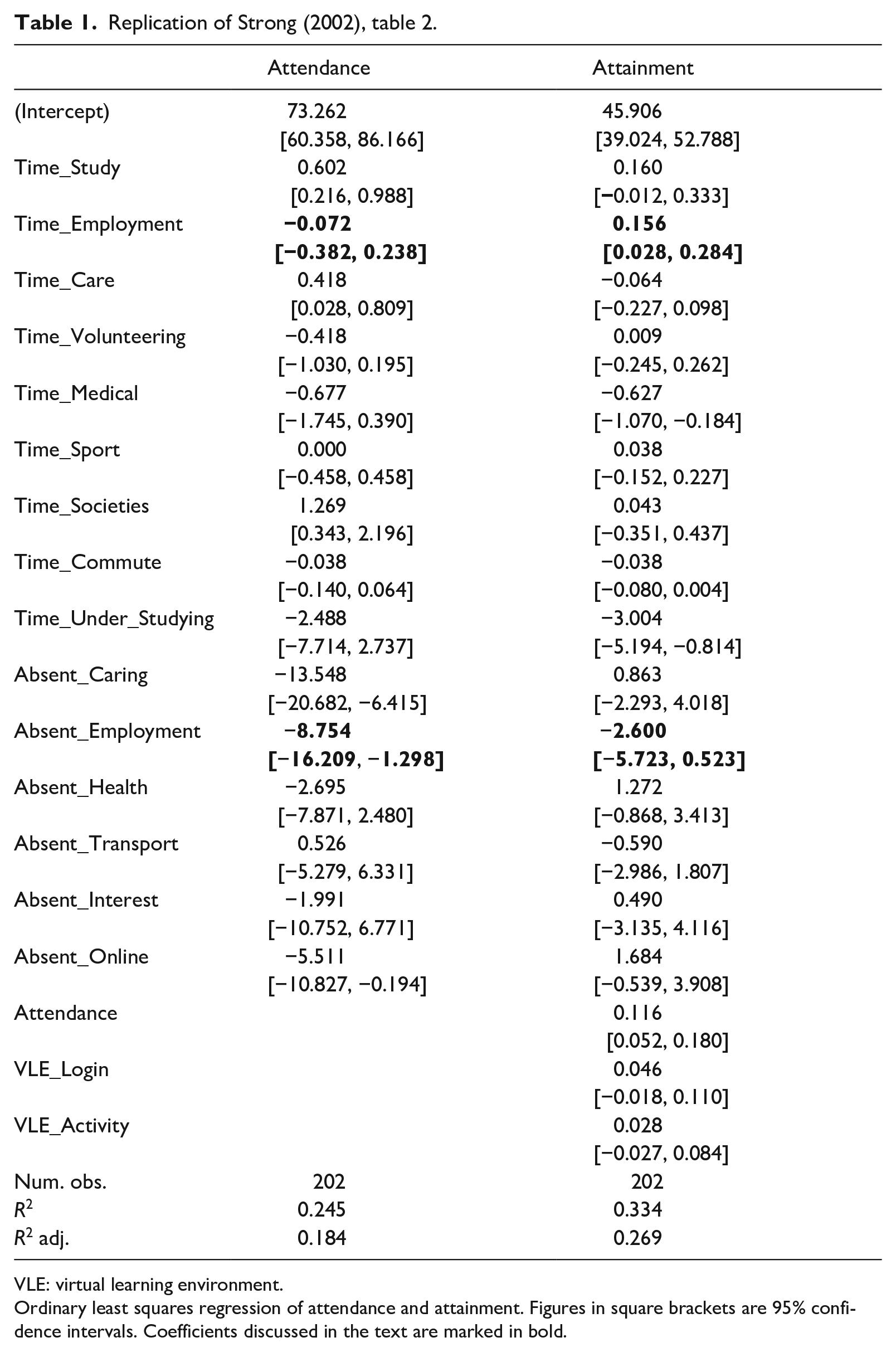
VLE: virtual learning environment.
Ordinary least squares regression of attendance and attainment. Figures in square brackets are 95% confidence intervals. Coefficients discussed in the text are marked in bold.
There is, however, another variable which is related to employment, and which does have a (statistically and substantively) significant effect on both attendance and attainment. That is, the variable which measures whether a student has ever missed a seminar due to a clash with employment (Absent_Employment). If a student has ever missed a seminar due to employment, their attendance is on average just under nine percentage points lower. (There is a negative effect on attainment, but it is not statistically significant).
The combination of these coefficient values is what warrants the overall conclusion that what matters is not ‘the absolute amount of time . . . [commitments like paid employment] require, but the fact they sometimes clash with taught classes’. In terms of the regression given in the left-hand column, values of the variable Time_Employment could increase by some number of hours without negatively affecting attendance, as long as values of the variable Absent_Employment did not change.
Why it is wrong
I argue that the regression coefficients in Table 1 do not support the overall conclusion of the article. Those coefficients cannot be interpreted as though they were causal effects, even under the most generous of assumptions, because the regression model includes a post-treatment variable, namely whether or not the student has ever missed a session due to a clash with paid employment. Crucially, this post-treatment variable is very closely associated with the outcome variable.
A post-treatment variable is a variable which is caused, either directly or indirectly, by a treatment variable, or some variable the effect of which we are interested in. In the regression models above, I consider ‘hours spent in paid employment’ to be the treatment variable, and ‘whether or not the student has ever missed a session due to a clash with paid employment’ as the post-treatment variable. The post-treatment variable is directly caused by the treatment variable: only students who are in employment can miss a session due to employment. 3 The post-treatment variable is also directly connected (by construction) to the outcome variable: students who missed a session due to paid employment cannot achieve perfect attendance, and would have attended a lower percentage of sessions than a student who was otherwise identical but who had not missed a session due to paid employment.
The inclusion of post-treatment variables in regression models means that the coefficients in these models cannot be interpreted as although they were causal effects. Montgomery et al. (2018) show this formally, but I can offer an intuitive account of why including post-treatment variables is wrong by giving an example. Many universities now produce information on their gender pay gap. Say a university produces statistics on gender pay gaps but produces these statistics separately by level of seniority. By controlling for, or conditioning on, seniority in this way, the university creates a false sense of the gender pay gap if gender affects seniority and if seniority affects salaries. The argument that ‘salaries are approximately equal looking at individuals of comparable seniority’ is not a defence if men are much more likely to be found in more senior positions. (This scenario is diagrammed on the left-hand side of Figure 1). In this case, gender affects salaries through promotion to more senior and more remunerative positions. There need not be any direct effect of gender on salary for gender to matter and for men to be advantaged.
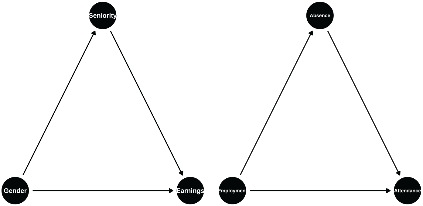
Example causal diagrams. Arrows indicate the direction of the causal effects.
The situation in Strong (2022) is exactly the same. Here, the number of hours a student spends in paid employment affects attendance through missing sessions. It is no defence of paid employment to say that ‘attendance is approximately equal between individuals who work many hours and few hours, looking at individuals who never missed sessions due to paid employment’. That, in essence, is what the regression model does. If anything, the situation is worse than in the gender pay gap example, because while it is possible to think of a world where gender does not matter for promotion, it is not possible to think of a world where paid employment is unconnected to missing sessions due to paid employment. By definition, only students who are in paid employment can miss a session due to paid employment. The two variables are necessarily connected.
What happens when we remove the post-treatment variable
The usual advice regarding the inclusion of post-treatment variables in regression is simply: ‘don’t do it’. Table 2 shows what happens if we take this advice. The table repeats the regression models shown in Table 1, except that now post-treatment variables are removed. This involves removing all of the variables marked as Absent_ in the model of attendance, and all of the variables relating to attendance from the model of attainment.
Analyses of attendance and attainment without post-treatment variables.
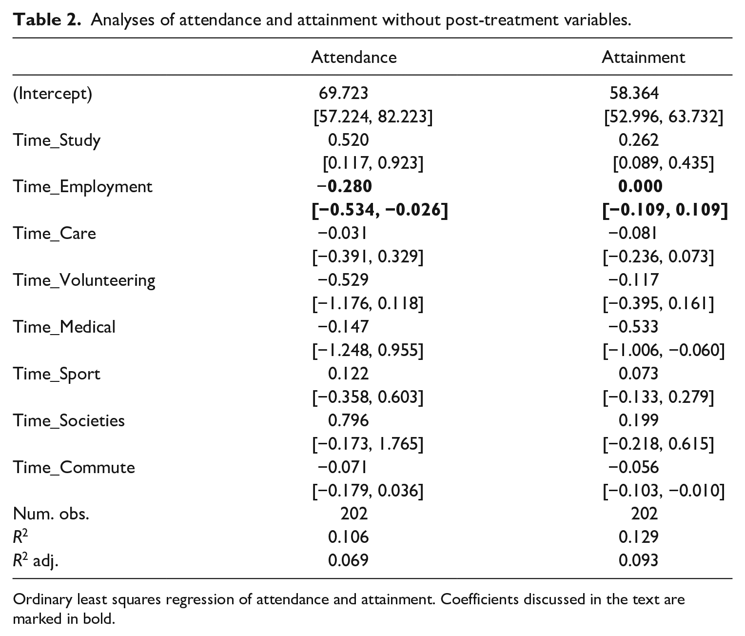
Ordinary least squares regression of attendance and attainment. Coefficients discussed in the text are marked in bold.
In the model in the left-hand column, the partial association between hours of employment and attendance is negative and significantly different from zero. An extra hour of work is associated with an attendance record which is lower by roughly one-quarter of one percentage point. Comparing two students who are scheduled to attend 60 teaching events over the course of a term, where one student works 20 hours a week and the other does not work at all, then we would expect the first student to attend three to four fewer sessions (20 × −0.0028 × 60 = −3.36) than the student who does not work. In the model of attainment, by contrast, the effect of hours of paid employment upon marks is not statistically significantly different from zero.
The coefficients in Table 2 can be interpreted as causal estimates of the effects of paid employment on attendance and attainment only if there are no omitted variables which affect both the hours of paid employment and attendance or both paid employment and attainment. This is unlikely to be the case. There are many variables which affect both hours of paid employment and attendance. Consider, as an example, ‘whether a student is a first-generation university student’. Past research has found that first-generation students tend to have lower rates of seminar attendance, even controlling for paid work (Oldfield et al., 2018). It seems likely that first-generation students will tend to work more, given that parents with a university education are likely to earn more, and parents who earn more tend to subsidise their children’s education more. 4 If we omit first-generation status from our regression, then the coefficient on paid employment will pick up a mixture of the effect of paid employment, and the effect of being a first-generation student. If we believe that the effect on attendance of a first-generation student is negative, then this means that the coefficient on paid employment will be more negative than the true effect of paid employment.
I have chosen ‘first-generation student’ as one particular omitted variable. Where there is only a single omitted variable, we can work out the direction of bias. Where there are multiple such variables, it is typically not possible to work out the direction of bias unless we know the relative importance of the omitted variables – and if we knew that, we likely would not face this problem to begin with.
What can be done to fix it
I have argued that the results of the regressions shown in Strong (2022) cannot be treated as estimates of the effect of paid employment upon attendance, and that for that reason it would be wrong to rely on this finding when framing academic policy or advising students. I have also presented a regression which I believe offers a closer approximation to the effect of paid employment upon attendance, but which also cannot be interpreted as a causal claim unless generous assumptions are made. What, as a practical matter, follows from this?
One option is to do an academic hair shirt, and insist that no action should be taken without causal identification, and that since none of the evidence presented herein can be interpreted causally, academics and university administrators should take no view on whether paid employment promotes or damages attendance. Only given appropriate evidence – perhaps a randomised controlled trial, where a sample of students already in employment is paid not to go in to work, would provide sufficient evidence.
A second option is to take the estimates in Table 2, and be willing to make bold assumptions regarding omitted variables – either that there are no such variables, or that the cumulative effect of these variables cancels out. This approach is unlikely to be defensible for an academic claim to knowledge, but might represent a practical approach driven by the need to adopt some view on the effects of paid employment on attendance, even if that view is decided only on the balance of probabilities.
A third option is to explore the sensitivity of the results in Table 2 to confounding of different degrees. Suppose that we combine all of the omitted variables into a single factor – an X-Factor, if you will. How big would this X-factor have to be, to make us change our conclusions about the deleterious effects of paid employment upon attendance?
We can assess this question by using the tools of sensitivity analysis. Sensitivity analysis allows us to see how the coefficient on time spent in employment changes as we make this ‘X-factor’ more or less tightly bound up with our outcome (attendance) and our treatment (hours spent in paid employment). Figure 2 is a contour plot, which shows the value of the coefficient on time spent in employment as we vary things about factor X. As we move left to right, our X-factor becomes more tightly bound up with time spent in employment – for example, first-generation students work much more than students whose parents went to university. As we move from bottom to top, our X-factor becomes more tightly bound up with attendance, such that first-generation students (or some other omitted group descriptor) are much less likely to attend. As a result, as we move towards the top or right of the graph, the value we would get for ‘time spent in employment’, if we could control for an X-factor of this kind, becomes smaller and smaller, and indeed starts becoming positive in the top-right two-thirds of the graph. This is shown by looking at the numbers plotted in grey on the contour lines.
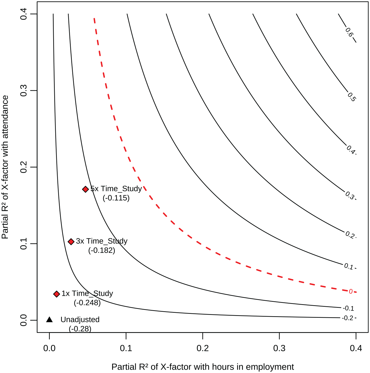
Contour plot showing the effect on attendance of hours in employment (contour lines) as a function of different levels of confounding.
The problem in interpreting this graph is that the coordinates on the horizontal axis are expressed in terms of partial R-squared, which is not an intuitive metric. To make this metric more intuitive, a series of ‘benchmarks’ are also plotted on the graph as red diamonds. The black triangle represents the current effect size. The diamonds above and to the right represent the effect of hours spent in employment if our X-factor had the same relationship to our treatment and outcome as ‘time spent studying’, or three times that strong a relationship, or five times that strong a relationship. Even if our ‘X-factor’ were
I take this to mean that it is unlikely that there is some unobserved factor (or set of factors) which would show a zero or positive effect of attendance. ‘Hours spent studying’ is the variable in the model of attendance in Table 2 which has the strongest relationship with attendance (partial R2 of 0.035). It is closely related to intrinsic motivation to study. The idea that there is some other variable out there which has a much stronger relationship with attendance seems difficult to imagine.
This is particularly true when considering factors that are within the control of university staff. To the extent that the model given in Table 2 does miss out on important predictors of attendance, these important predictors seem much more likely to be sociodemographic in nature. Whether or not a student has a parent who went to university seems likely to have a large effect on attendance. By comparison, the effect of timetabling seems as though it is likely to be minor.
What are the implications of this?
I view the implications of this as two-fold. First, there are implications for our knowledge of the determinants of attendance. We should (continue to) believe that paid employment has a negative effect on attendance. For many academics, this will not be hard, as this belief is intuitive. Our knowledge is imperfect, because although we should be fairly confident regarding the sign of this relationship, it is much harder to assess the strength of this relationship. In the model shown in Table 2, each extra hour of paid employment is associated with levels of attendance that are one-quarter of one percentage point lower. However, if there are other factors out there that simultaneously (positively) affect paid employment and (negatively) affect attendance, then the size of this effect might be smaller. For example, each extra hour of paid employment might be associated with levels of attendance that are one-tenth of one percentage point lower (top-right point plotted in Figure 1).
Second, there are implications for how we relate to students. To some extent, what academics say about studying affects what students do. There is a risk that students who are told that ‘paid work negatively affects attendance’ will believe this claim and act differently because they believe this claim. The risk of this happening is low: our ability to shape our students’ behaviour is not that great. However, it would be unfortunate if these findings, when repeated to students, became self-fulfilling.
At the same time, academics do have some obligations to candour, and certainly, if our students ask whether paid employment is likely to damage their attendance, we should be honest with them and acknowledge that there are trade-offs. It is possible to acknowledge uncertainty – even the best-designed experimental trial only ever identifies average treatment effects, and it is possible that the effects on some students will be closer to zero. But, it is unlikely that the average effects are so benign.
Ultimately, the surest ground for any conversation with students is to return to what we as academics know best, namely the demands of the course. If we believe we know how much work our course requires per week, and if this workload is consistent with a full-time position in education, then we should communicate this expectation to our students, and leave them to work around it.
Footnotes
Funding
The author(s) received no financial support for the research, authorship and/or publication of this article.