Sage Journals: Discover world-class research

Abstract

The main objective of this paper is to determine the effect of outer race defect of deep groove ball bearings for (SKF 6004) through experimental and numerical methods. Three-dimensional finite element model of the housing and outer race is simulated using commercial package ABAQUS/CAE. Angular position of the local defect on the outer race which changes from 0° to 315° with angular intervals 45° is investigated through the dynamic finite element model. Experimental results are obtained using bearing test rig to validate the simulated results. A good agreement is found between the results obtained by the finite element model and the experimental results.

Keywords

Vibration analysis dynamic modelling

Introduction

Rolling bearing damage may result in a complete failure of the rolling bearing or at least, a reduction in operating efficiency of the bearing arrangement. Bearing damage does not always originate from the bearing alone. Damage due to bearing defects in material or workmanship is exceptional. Vibration analysis is among the most common methods used in monitoring applications since a defect produces successive impulses at every contact of defect and the rolling element, and the housing structure is forced to vibrate at its natural modes.

The use of statistical moments of the rectified data has been compared to the moment of the original data.¹ By using the estimated frequency, a simple notch filter removes the frequency component so that further detail in the vibration signal may be analysed.² An alternative framework for analysing bearing vibration signals, based on cyclostationary analysis, has been proposed.³ The synchronous averages are used to examine the calculation of the envelope signal of the high-frequency vibration produced by rolling element bearings with spalling damage.⁴ The effect of local defects on the nodal excitation functions is modeled. Vibration signals are obtained using simulation method.⁵ Furthermore, both inner and outer race defects were artificially introduced to the bearing using electrical discharge machining.⁶ The defect was detected using off-the-shelf portable vibration analysis hardware and software.⁷

A complex filter for Hilbert transform is proposed to apply in real-time vibration signal demodulation. Thus, a finite waveform interval of the proposed filter could be possibly applied in the vibration signal demodulation.⁸ Time domain, frequency domain analysis and spike energy analysis have been employed to identify different defects in bearings.⁹ Statistical properties of the vibration signals for healthy and defected structures are compared.¹⁰ Time-domain parameters such as root mean square (RMS), crest factor and kurtosis are used to analyse the vibration signals.^11,12 The simulated vibration pattern has similar characteristics with results from experimental results.¹³ Then, the model is analysed to obtain the vibration signal in the frequency domain.¹⁴

The finite element (FE) model is proposed to study ball bearing with local defect based on the coupling of piecewise function and contact mechanism at the edge of the local defect.^15–18 An analytical model is proposed to study the non-linear dynamic behaviour of rolling element bearing systems including surface defects.¹⁹ The vibrations generated by deep groove ball bearings having multiple defects on races were studied.²⁰ A simple time series method for bearing fault feature extraction using singular spectrum analysis of the vibration signal is proposed.²¹ The resonance frequency in the first vibration mode of mechanical system was studied.²² Under the assumption of a stepwise function for the envelope signal, the modulated signal could be decomposed into a sinusoidal function basis at the first vibration mode resonance frequency. A mathematical model for the ball bearing vibration due to defect on the bearing race has been developed.²³

The aim of this study is to model a deep groove ball bearing and to obtain simulated vibration signals of outer race defect using FE analysis through ABAQUS software. The effect of defect on the outer race and its angular position is investigated. The vibration monitoring methods are examined using statistical parameters such as RMS, crest factor, kurtosis and skewness.

Dynamic model of vibration data

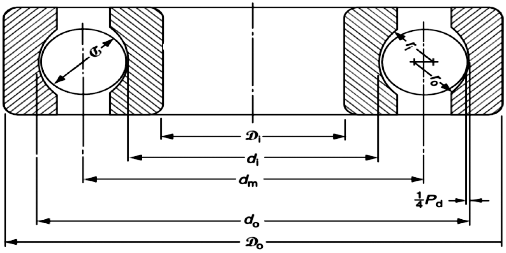
In this study, a single row deep groove ball bearing is used. The bearing geometry is shown in Figure 1 and its dimensions are:

Outer diameter D_o = 42 mm

Bore diameter D_i = 20 mm

Pitch diameter d_m = 31 mm

Raceway width B = 12 mm

Ball diameter D = 6.35 mm

Contact angle α = 0°

Number of balls Z = 9 balls

Raceway diameter of outer race d_o = 34.8 mm

Raceway diameter of inner race d_i = 27.2 mm

Figure 1.

Geometry of the deep groove ball bearing 6004.²⁴

In this study, a 6004 model single row deep groove ball bearing with stationary outer ring and housing are considered. It is assumed that the contact between the outer surface of the outer ring and its mating surface on the casing structure is perfect meaning that no relative motion is permitted on the contact surface. The three-dimensional models of the housing and outer ring are constructed in commercial package ABAQUS/CAE which is used in different applications.^25–27 The housing model is created according the dimensions shown in Figure 2. The outer race dimensions of the SKF 6004 ball bearing are used. It is also assumed that the bearing material is isotropic and linear-elastic fracture mechanics with modulus of elasticity “E” of 203 GPa, Poisson’s ratio “ν” of 0.29 and density “ρ“ of 7850 kg/m³. For the housing, the material is assumed to be isotropic and linear-elastic fracture mechanics with modulus of elasticity “E” of 195 GPa, Poisson’s ratio “ν” of 0.26 and density “ρ“ of 7300 kg/m³.

Figure 2.

Basic dimensions of the housing structure (dimensions in mm).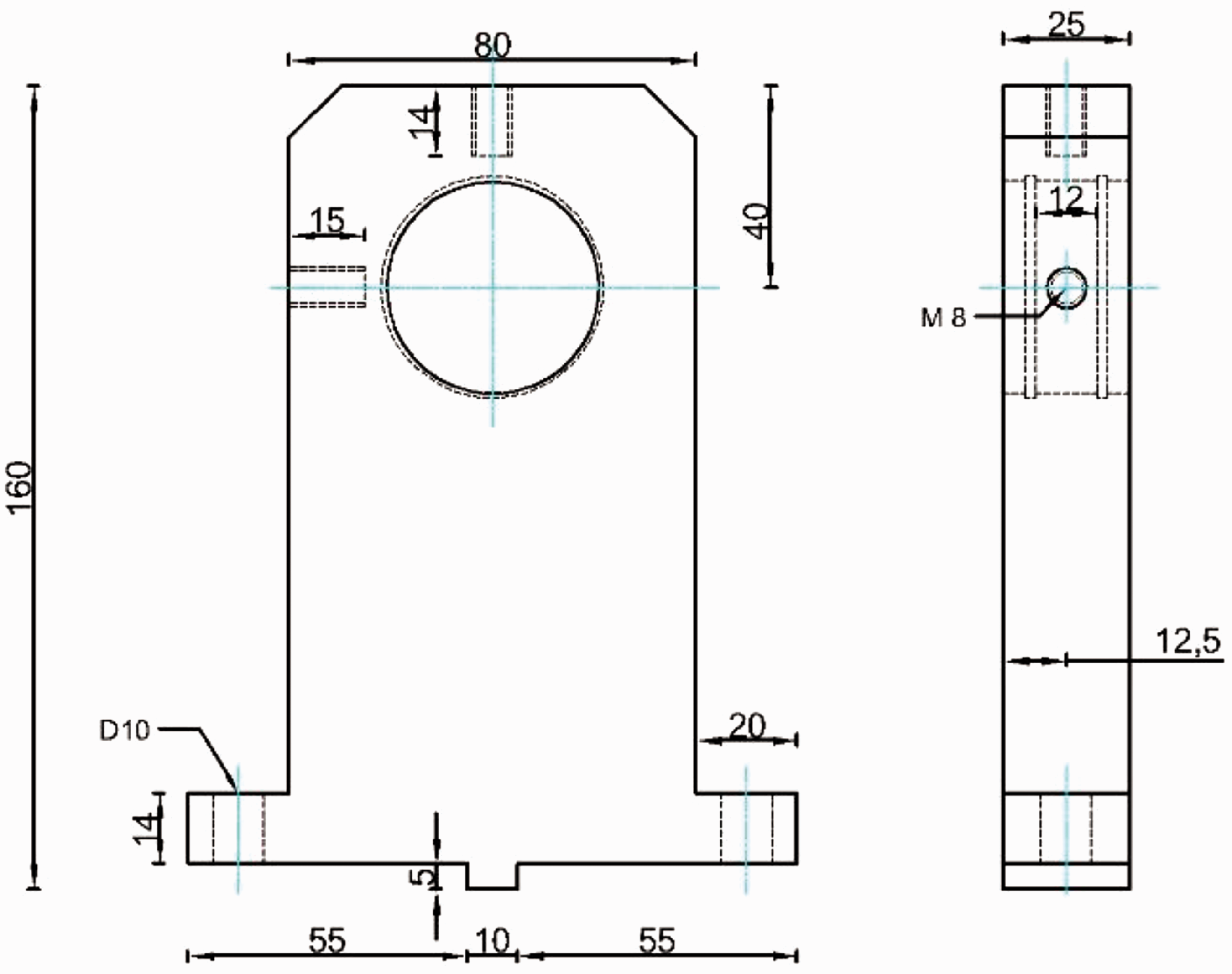

Figure 3 shows the dynamic model with two set measure points, P1 and P2, on which the frequency will be determined. The inner surface of the housing hole and the outer surface of the bearing outer race are defined as tie constrains. The housing part is fixed in three mutual perpendicular displacement directions (U1, U2, U3); mainly x-, y- and z-directions; as well as it is non-rotational about these axes (UR1, UR2, UR3). The load acting on each node along the inner circumference of the loading zone of the outer raceway has to be developed. The mesh of explicit elements with reduced integration and eight nodes (C3D8R) are used. Both housing and race are defined with the element type but using different global sizes.

Figure 3.

Three-dimensional model of the housing with outer race of bearing.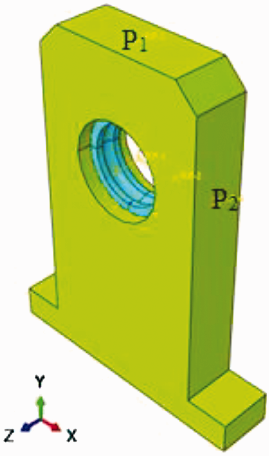

Load distribution

The loads carried by the ball and roller bearings are transmitted through the rolling elements from one ring to the other.²⁴ The relationship between load and deflection is

Q = K δ n

(1)

where “n” = 1.5 for ball bearings and “n” = 1.11 for roller bearings, “Q” is the ball or roller normal load, “δ” is deformation and “K” is load-deflection factor.

For a rigidly supported bearing subjected to a radial load, the radial deflection at any rolling element angular position is given by

δ_{ψ} = δ_{\max} [1 - \frac{1}{2 ɛ} (1 - \cos ψ)]

(2)

ɛ = \frac{1}{2} (1 - \frac{P_{d}}{2 δ_{r}})

(3)

where “δ_max” is the maximum race radial shift, occurring at ψ = 0⁰, “ψ” is azimuth angle, “P_d” is the diametric clearance, “ɛ” is the load distribution factor.

The angular extent of the load zone is determined

ψ_{l} = \cos - 1 \frac{P_{d}}{2 δ_{r}}

(4)

For ball bearings having zero clearance and subjected to a simple radial load it may be determined that

Q_{ψ} = Q_{\max} [1 - \frac{1}{2 ɛ} (1 - \cos ψ)] n

(5)

Q_{\max} = \frac{4.37 F_{r}}{Z \cos α}

(6)

where “F_r” is radial load and “Z” is number of balls.

One of the simpler detection and diagnostic approaches is to analyse the measured vibration signal in the time domain. Whilst this can be as simple as visually looking at the vibration signal, other more sophisticated approaches can be used such as trending time domain statistical parameters. A number of statistical parameters can be defined as RMS, peak, crest factor, kurtosis and skewness based upon beta distribution.

Time domain statistical parameters have been used as one-off and trend parameters in an attempt to detect the presence of incipient bearing damage. The vibration data are calculated for vertical and horizontal directions for a broad range of rotational speed ranging from 1500 to 3500 r/min

RMS = \sqrt{\frac{1}{N} \sum_{i = 1}^{N} [X (t) - \bar{X}]}

(7)

Crest factor = [\max . (X) - \min . (X)] / RMS

(8)

Kurtosis = \frac{1}{N} \sum_{i = 1}^{N} [X (t) - \bar{X}] 4 / RMS 4

(9)

Skewness = \frac{1}{N} \sum_{i = 1}^{N} [X (t) - \bar{X}] 3 / RMS 3

(10)

where

\bar{X}

denotes the mean value of the discrete time signal X(t) having N data points.

The magnitude and duration of the impulse force are related with the radial load carried by the outer race defect and the velocity of the rolling elements. A local defect is modelled by amplifying the magnitudes of the radial forces defined for the nodes which are in the defected area. The amplification constant is chosen simply as 3.58, in this study. The outer race defect frequency (defect on outer race) is given as

f_{o} = \frac{{Zf}_{s}}{2} (1 - \frac{D}{d_{m}} \cos α)

(11)

According to equation (11), the relation between the outer race defect frequency and the shaft frequency is given as

f_{o} = 3.58 f_{s}

Experimental setup

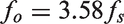
An experimental setup is employed in this work to collect the vibration signals to study the vibration signatures, generated by incipient bearing defects. The test rig and the equipment used in collecting the data are shown in Figure 4. The system is driven by a variable motor with speed up to 6000 r/min. An optical encoder is used for the speed measurement. An elastic claw coupling is utilized to damp out the high-frequency vibration generated by the motor. Two ball bearings are fitted into the solid housings. Accelerometers (IMI Sensors-603C01) are mounted on the housing of the tested bearing to measure the vibration signals along two directions. A variable load is applied by a belt drive, where the signal collection is carried out by a data acquisition card.

Figure 4.

Schematic representation of the test rig.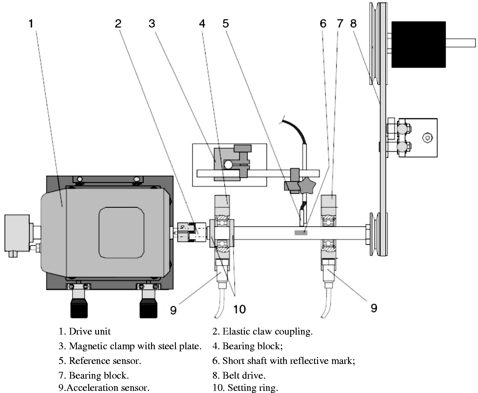

Validation between the experimental and simulation results

The boundary conditions of the simulation process have been chosen to satisfy an acceptable homogeneity between the experimental setup and the simulated model. Figure 5 shows an experimental acceleration signal for a healthy bearing and a bearing with a defected outer race, while the corresponding signal that was obtained from the simulation process is shown in Figure 6. It is observed from Figures 5(a) and 6(a) that the dynamic response of the healthy bearing is approximately similar for the experimental and theoretical cases.

Figure 5.

Experimental acceleration signals for bearings (a) healthy bearing and (b) bearing with defected outer race.

Figure 6.

Numerical acceleration signals for bearings (a) healthy bearing and (b) bearing with defected outer race.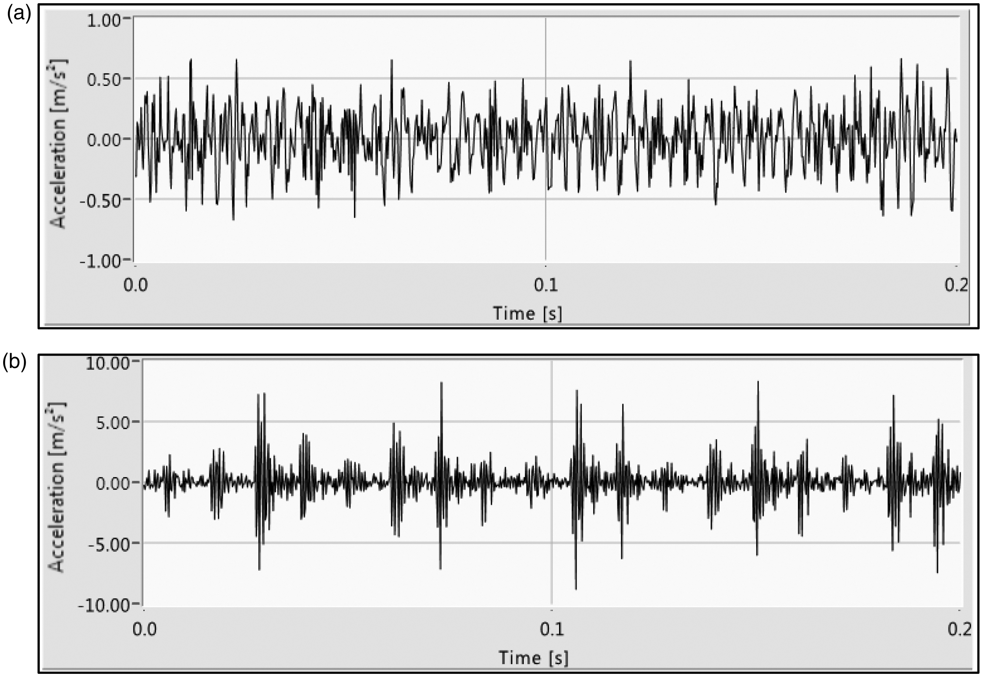

Furthermore, it is noticed for the case of bearing with defected outer race that the experimental results of Figure 5(b) confirm that of the defected bearing, i.e. Figure 6(b). These results indicated that the proposed method of simulation can be used to produce vibration data for condition-monitoring applications. However, the difference between the experimental and simulation signals may be due to the interval time used in dynamic model which has the value of 0.0001 s, where the interval time used in experimental test which has the value of 0.01 s.

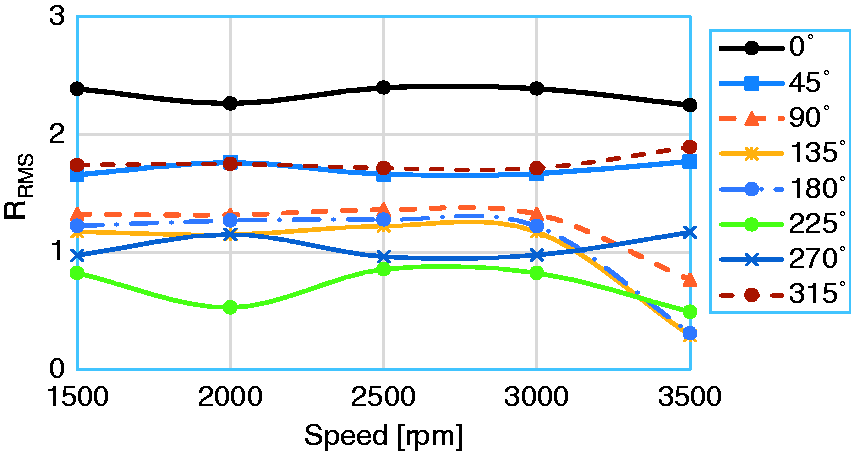
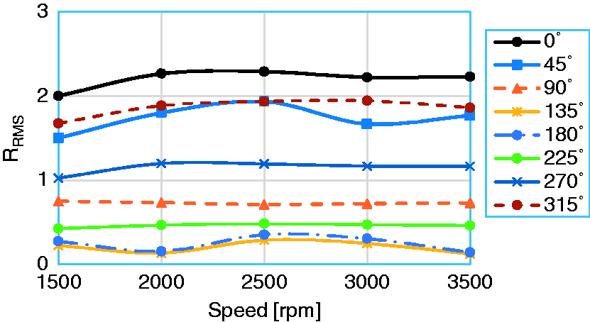
The experimental results investigate the ratio between the RMS of the acceleration of the defected bearing to that of the healthy one “R_RMS.” Figure 7 illustrates the RMS-ratio of the acceleration “R_RMS” for bearing with outer race defect versus the shaft speed. The RMS-ratio in the vertical direction displays higher values than that of the horizontal direction. Also, the value of the RMS-ratio decreases with the increase of the shaft speed. It is important to notice that the higher values of the RMS-ratio on the vertical direction are connected to the position of the defect of the outer race, which means that the RMS-ratio increases at the position of the outer race defect.

Figure 7.

Experimental variation of the acceleration RMS-ratio versus shaft speed for bearing with outer race defect.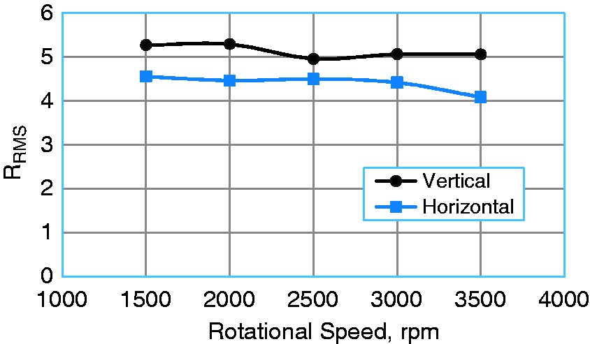

The analytical result describes the alteration of the bearing acceleration, velocity and displacement. Figure 8 illustrates the variation of the RMS-ratio of the acceleration versus the shaft speed. The value of the RMS-ratio at point “P₁,” i.e. in the vertical direction is small in comparison to the horizontal one. Also, the RMS-ratio decreases with the increase of the shaft speed. Therefore, it is easier to detect the bearing defect at low speeds than that by high speeds which can be due to the reduction of the pulse interval. The comparison between the simulation and experiment results shows a good agreement between the results. However, the variation between the experimental and the simulation values may be due to the inequality of the defect size in both cases.

Figure 8.

Analytical variation of the acceleration RMS-ratio versus shaft speed for bearing model with outer race defect.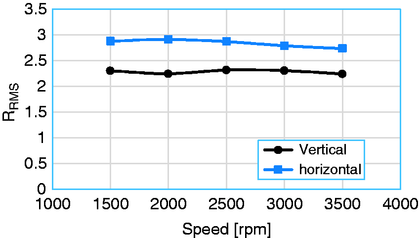

Effect of the defect position on the outer race

The vibration data are calculated for points P₁ and P₂ for a broad range of rotational speed ranging from 1500 to 3500 r/min. The RMS-ratio “R_RMS” is the ratio between the RMS of the defected bearing to that of the healthy one. The crest factor ratio “C_CF” is the ratio between the crest factor parameter “CF” of the defected bearing to that of the healthy one. The kurtosis ratio “K_K” is the ratio between the kurtosis parameter “K” of the defected bearing to that of the healthy one. The skewness ratio “S_S” is the ratio between skewness parameter “S” of the defected bearing to that of the healthy one.

The analytical results describe the alteration of the bearing acceleration response as shown in Figure 9. It can be seen that the RMS-ratio of the acceleration “R_RMS” with positive clearance, 0 < ɛ < 0.5, gives the high result with low speed. It can be observed for the zero clearance, ɛ = 0.5, and the negative clearance or preload, 0.5 < ɛ < 1, that the RMS-ratio of the acceleration “R_RMS” is almost constant for all speeds. It can be concluded that the RMS-ratio of the acceleration “R_RMS” increases due to the increase of the clearance value. The same observation is valid for displacement and velocity responses.

Figure 9.

RMS acceleration response of the bearing clearance for bearing model.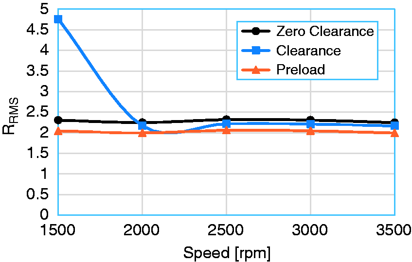

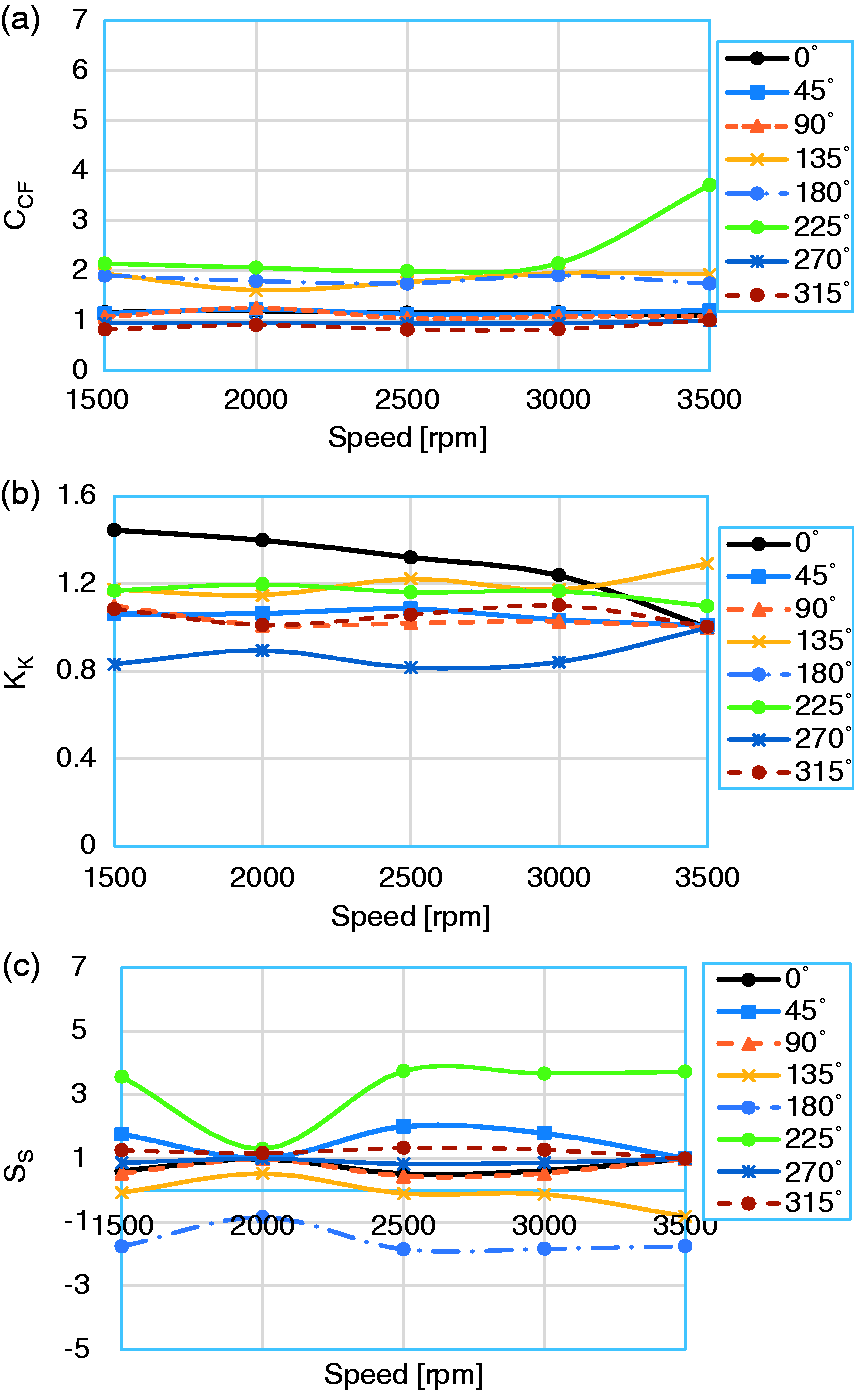
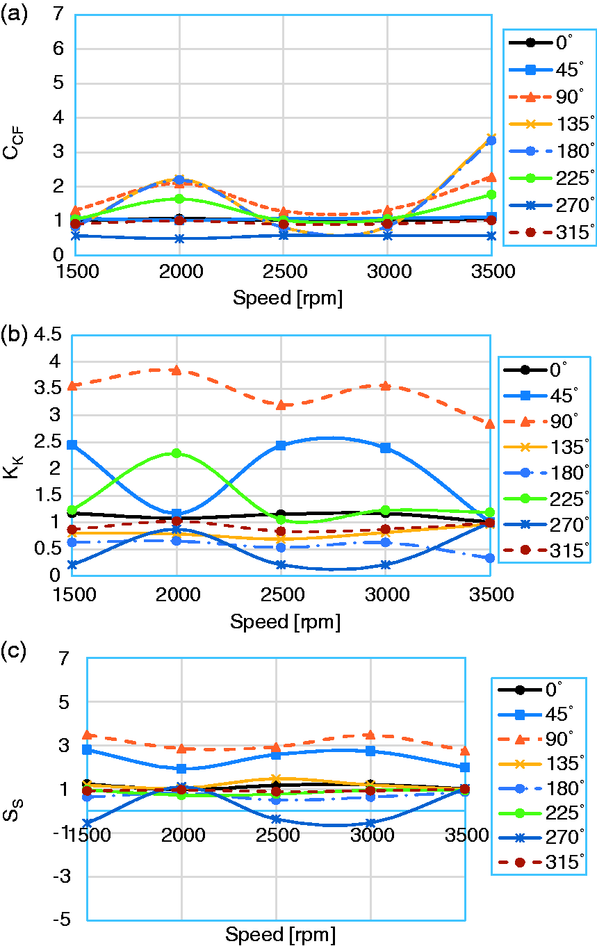
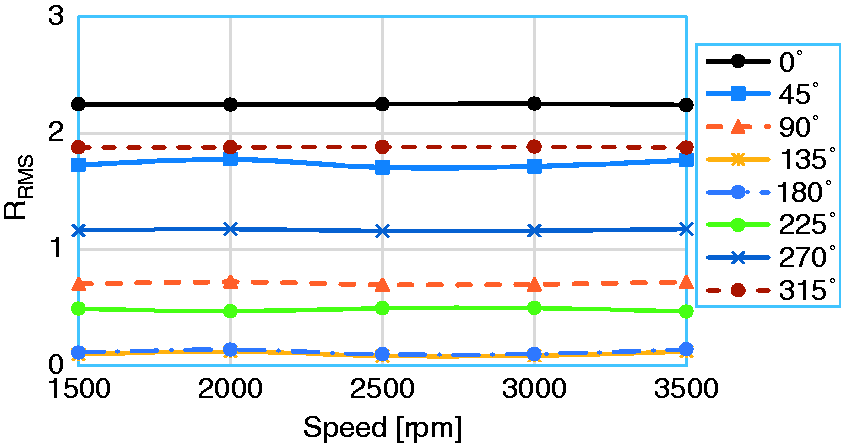
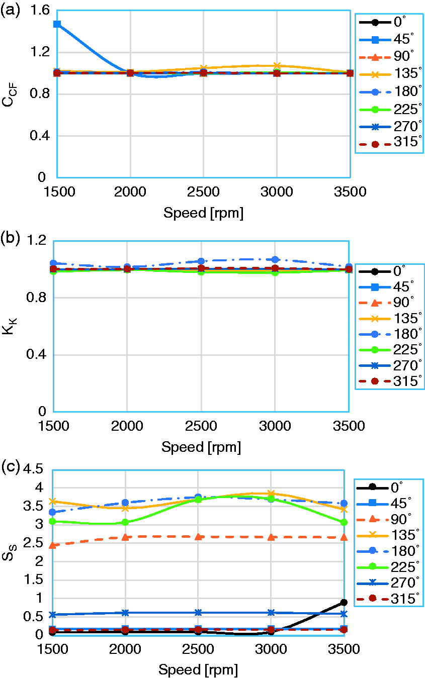
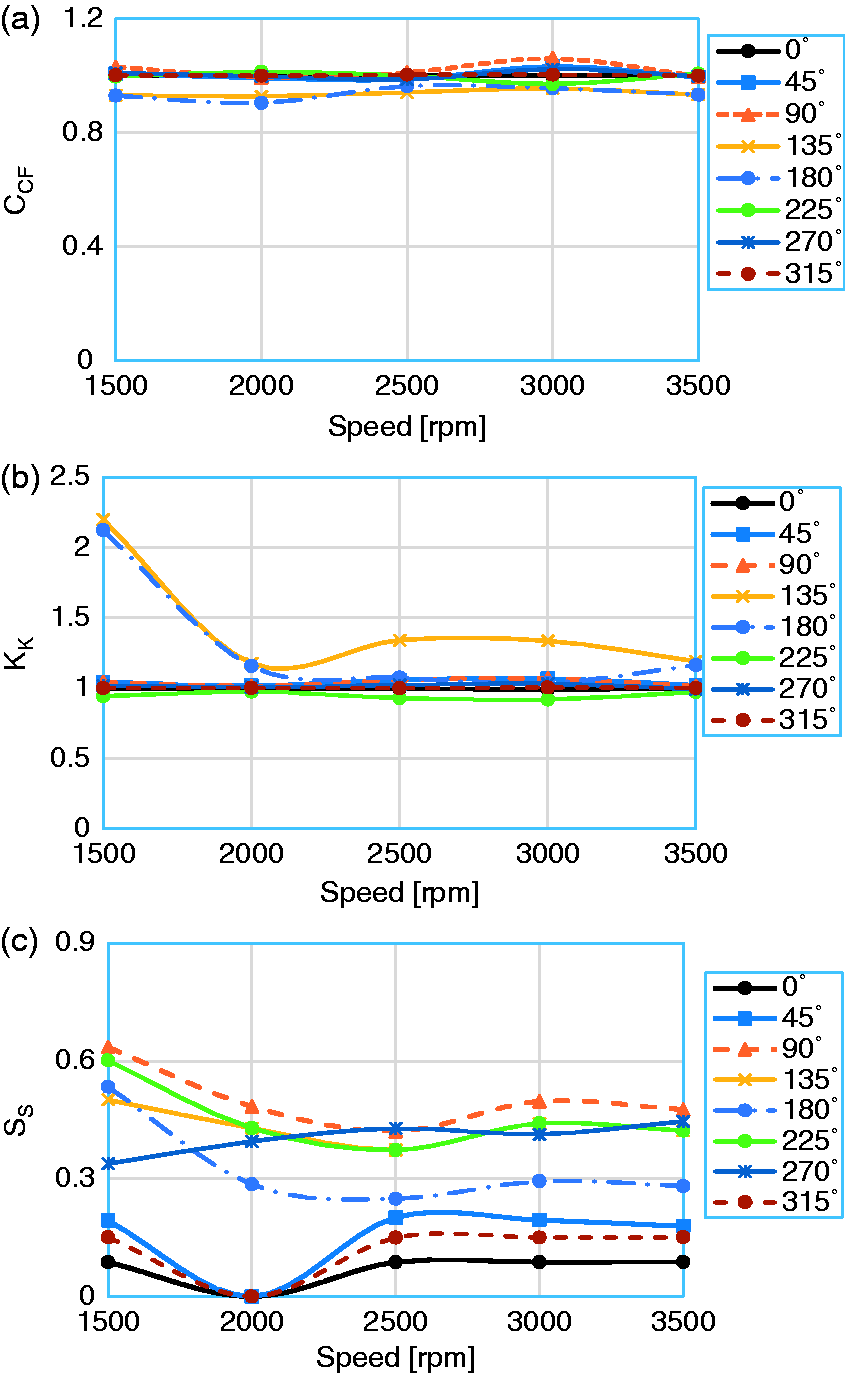
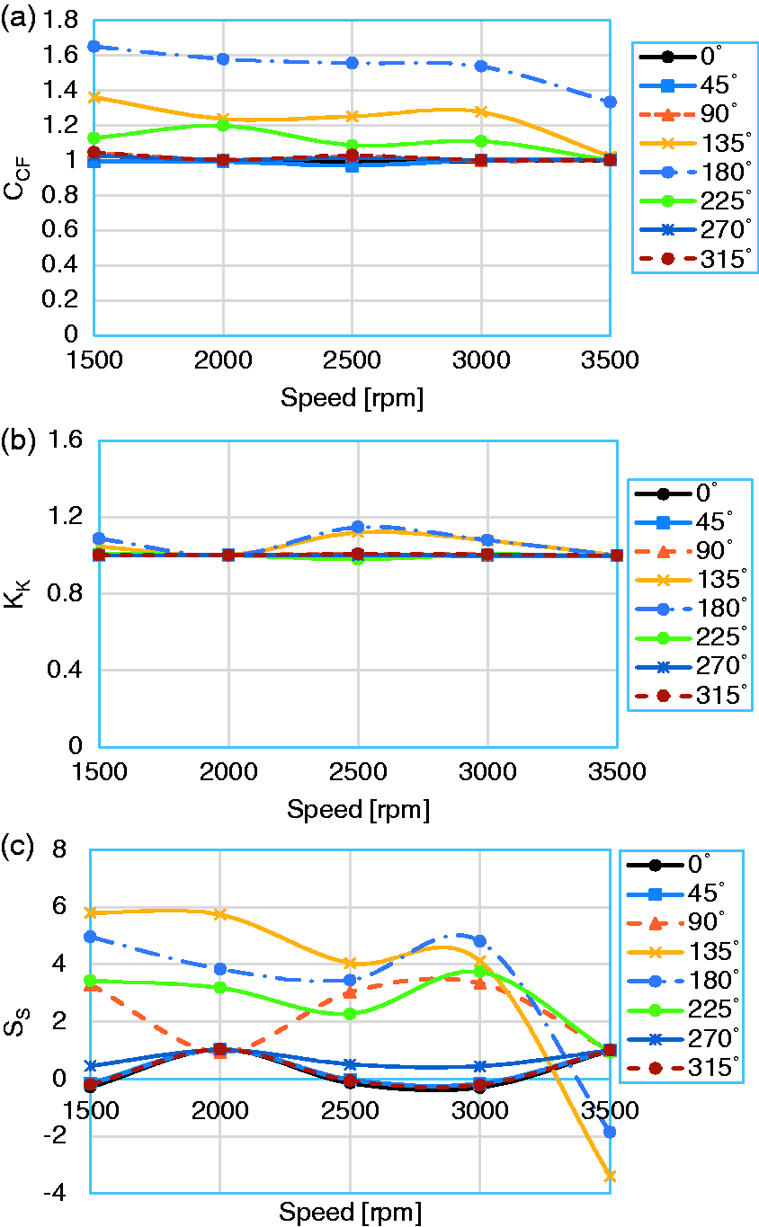
The analytical results describe the alteration of bearing acceleration, displacement and velocity for vertical and horizontal directions. It can be seen from Figure 10 that the RMS-ratio “R_RMS” at point “P₁,” i.e. in the vertical direction gives high result with the defect located at 90°. While the low result is given with the defect located at 135°, 180° and 225°, a local defect at 0° gives high result at point “P₂,” i.e. in the horizontal direction as shown in Figure 11. Furthermore, as local defect at 225° gives the low result and the defects located at 45° and 315° give the same result, it can be concluded that the point “P₂,” i.e. in the horizontal direction is a good sensor location to detect a local defect at 0° according the RMS-ratio result. And also, point “P₁,” i.e. in the vertical direction is a good sensor location to detect a local defect at 90°. Furthermore, the defects located at the radial load distribution area have more effect than the defects located at the unloaded area. Figure 12(a) illustrate the crest factor ratio “C_CF” for the acceleration of the bearing model at point “P₁,” i.e. in the vertical direction. It can be observed that the crest factor ratio “C_CF” has low result with the defects which is located at the loaded area. However, the defects located at the unloaded area, 135° – 180° – 225°, give the high results. It can be concluded that the crest factor ratio seems to be a better parameter for defects located at the unloaded area. The kurtosis ratio for acceleration “K_K” at point “P₁,” i.e. in the vertical direction is shown in Figure 12(b). A local defect at 0° gives high result at relatively low speeds. And also, a local defect at 270° gives the low result and the defects located at 135° and 225° give the same result. It can be seen from Figure 12(c) that a local defect at 225° gives the high result and the defect located at 180° gives low result. The defects at the other locations are difficult to monitor by using the skewness ratio “S_S” calculated from the acceleration results for point “P₁,” i.e. in the vertical direction. The crest factor ratio “C_CF” for the acceleration of the bearing model at point “P₂,” i.e. in the horizontal direction is shown in Figure 13(a). It can be observed that crest factor ratio “C_CF” is very small for all speeds and it is difficult to detect a defect by using the crest factor results. It can be concluded that the horizontal point is not suitable during defect detection for the crest factor. A local defect at 90° gives high result for the kurtosis ratio “K_K” at point “P₂,” i.e. in the horizontal direction as shown in Figure 13(b). Furthermore, a local defect at 270° gives the low result. The same observation is valid for the kurtosis and skewness ratios.

Figure 10.

Acceleration RMS-ratio of defect positions at point “P₁.”

Figure 11.

Acceleration RMS-ratio of defect positions at point “P₂.”

Figure 12.

Acceleration ratios of defect positions at point “P₁.” (a) Crest factor, (b) kurtosis and (c) skewness.

Figure 13.

Acceleration RMS-ratio of defect positions at point “P₂.” (a) Crest factor, (b) kurtosis and (c) skewness.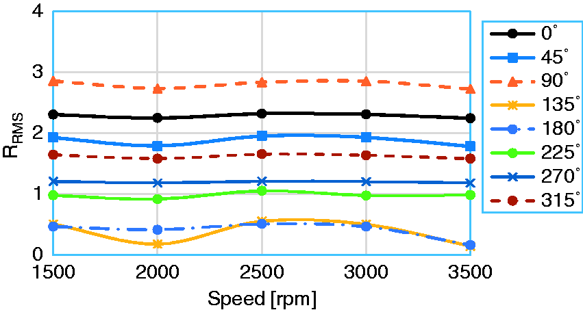

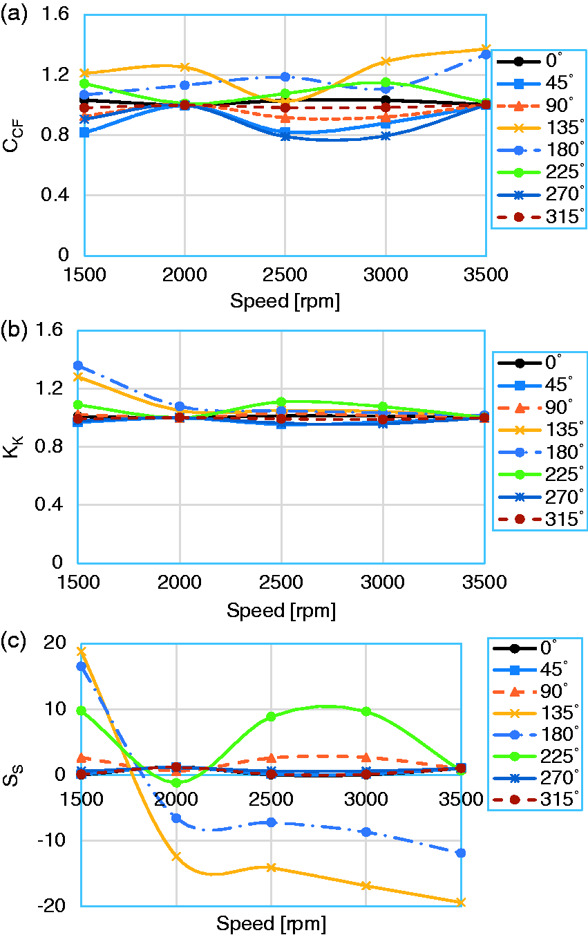
The RMS-ratio of the displacement “R_RMS” at point “P₁,” i.e. in the vertical direction is shown in Figure 14. It can be noticed that the RMS-ratio gives high result with the defect located at 90°, while the low result is given with the defect located at 135°, 180° and 225°. Furthermore, a local defect at 0° gives high result at point “P₂,” i.e. in the horizontal direction; local defect at 225° gives the low result as shown in Figure 15. It can be concluded that the horizontal direction is a good sensor location to detect a local defect at 0° according the RMS-ratio results. And also, the point “P₁” is a good sensor location to detect a local defect at 90°. It can be seen from Figure 16(a) and (b) that the crest factor and kurtosis ratios at point “P₁,” i.e. in the vertical direction are very small for all speeds and it is difficult to detect a defect. However, the defects located at the unloaded area, 135° – 180° – 225°, give the high results at the skewness ratio as shown in Figure 16(c). The same observation of the crest factor at point “P₁,” i.e. in the vertical direction is valid for the point “P₂,” i.e. in the horizontal direction. A local defect at 135° and180° gives high result at relatively low speeds by using the kurtosis ratio. It can be observed from Figure 17(c) that the skewness ratio of the defected bearings is less than healthy bearings for all speeds. It can be concluded that the crest factor and kurtosis ratios for the displacement are not suitable during defect detection, while the skewness ratio is suitable during defect detection for the defects located at the unloaded area.

Figure 14.

Displacement RMS-ratio of defect positions at point “P₁.”

Figure 15.

Displacement RMS-ratio of defect positions at point “P₂.”

Figure 16.

Displacement ratio of defect positions at point “P₁.” (a) Crest factor, (b) kurtosis and (c) skewness.

Figure 17.

Displacement ratios of defect positions at point “P₁.” (a) Crest factor, (b) kurtosis and (c) skewness.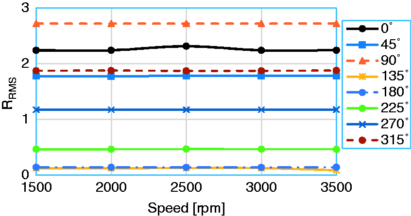

The RMS-ratio for the velocity responses at vertical and horizontal directions is shown in Figures 18 to 21. It can be noticed that the same observation is valid for displacement and velocity responses for the RMS-ratio. It can be seen from Figure 20(a) that the crest factor ratio at point “P₁,” i.e. in the vertical direction gives high result with the defects located at 180°and 270°, respectively, while all the other defects have no great effect. It can be seen from Figures 20(b) and 21(b) that the kurtosis ratio at point “P₁,” i.e. in the vertical direction is very small for all speeds and it is difficult to detect a defect. It can be noticed that the same observation is valid for the crest factor parameter at the point “P₂,” i.e. in the horizontal direction. It can be observed in Figure 20(c) that the skewness ratio at vertical direction gives high result with the defects located at 270°, 180° and 225°. Furthermore, a local defect at 90° gives high result at point “P₁,” i.e. in the vertical direction, with all speeds except 2000 r/min. However, the defects located at 270° and 180° give the high results at the skewness ratio as shown in Figure 20(c). It can be concluded that the kurtosis ratio for the velocity response is not suitable during defect detection, while the skewness ratio is suitable during defect detection for the defected located at the unloaded area.

Figure 18.

Velocity RMS-ratio of defect positions at point “P₁.”

Figure 19.

Velocity RMS-ratio of defect positions at point “P₂.”

Figure 20.

Velocity ratios of defect positions at point “P₁.” (a) Crest factor, (b) kurtosis and (c) skewness.

Figure 21.

Velocity ratios of defect positions at point “P₂.” (a) Crest factor, (b) kurtosis and (c) skewness.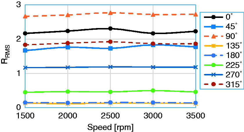

Conclusions

Based on the results obtained from the corrected FE model, the following conclusions can be drawn:

Good agreement is found between the results obtained by ABAQUS/CAE and the experimental results.

According to the RMS parameter for all time responses, the increase in the ratio between the time domain parameters of the defected and healthy bearings is due to the increase of the clearance value.

The defects located at the radial load distribution area have more effect than the defects located at the unloaded area.

The crest factor and kurtosis ratios for displacement and velocity response are not suitable during defect detection, while the skewness ratio is suitable during defect detection for the defect located at the unloaded area.

Footnotes

Declaration of conflicting interests

The author(s) declared no potential conflicts of interest with respect to the research, authorship, and/or publication of this article.

Funding

The author(s) received no financial support for the research, authorship, and/or publication of this article.

References

Farhang H. An investigation into rolling element bearing failure analysis. PhD Thesis, The University of Waterloo, Canada, 1992.

Wang Y-F and Kootsookos PJ. Frequency estimation in the fault detection of rolling element bearing. In: Fifth international congress on sound and vibration, Adelaide, Australia, 15–18 December 1997.

Antoniadis

Glossiotis

. Cyclostationary analysis of rolling-element bearing vibration signals. J Sound Vibr 2001; 248: 829–845.

Mcfadden

Toozhy

. Application of synchronous averaging to vibration monitoring of rolling element bearings. Mech Syst Signal Process 2000; 14: 891–906.

Kiral Z. Simulation and analysis of vibration signals generated by rolling element bearings with defects. PhD Thesis, The University of Izmir, Turkey, 2002.

Ocak

Loparo

. Estimation of the running speed and bearing defect frequencies of an induction motor from vibration data. Mech Syst Signal Process 2004; 18: 515–533.

Johnson

Jr . Vibration tests for bearing wear. ASHRAE J 2000; 42: 52–56.

Sheen

Y-T

. A complex filter for vibration signal demodulation in bearing defect diagnosis. J Sound Vibr 2004; 276: 105–119.

Amarnath

Shrinidhi

Ramachandra

. Prediction of defects in antifriction bearings using vibration signal analysis. IE (I) Journal-MC 2004; 85: 88–92.

10.

Kiral

Karagulle

. Simulation and analysis of vibration signals generated by rolling element bearing with defects. Tribol Int 2003; 36: 667–678.

11.

Karacay

Akturk

. Experimental diagnostics of ball bearings using statistical and spectral methods. Tribol Int 2009; 42: 836–843.

12.

Kim Y-H, Tan ACC, Mathew J, et al. Condition monitoring of low speed bearings: a comparative study of the ultrasound technique versus vibration measurements. In: Proceedings of world congress on engineering asset management (WCEAM), Gold Coast, Australia, 11–14 July 2006. London: Springer, pp.182–191.

13.

Kadarno P and Taha Z. Vibration analysis of defected ball bearing using finite element model simulation. In: The 9th Asia Pacific industrial engineering & management systems conference, Bali, Indonesia, 3–5 December 2008.

14.

Taha Z and Dung NT. Rolling element bearing fault detection with a single point defect on the outer raceway using FEA. In: The 11th Asia Pacific industrial engineering & management systems conference, Melaka, Malaysia, 7–10 December 2010.

15.

Liu

Shao

Lim

. Vibration analyses of ball bearings with a localized defect applying piecewise response function. Mech Mach Theory 2012; 56: 156–169.

16.

Cao

Niu

. Method for vibration response simulation and sensor placement optimization of a machine tool spindle system with a bearing defect. Sensors 2012; 12: 8732–8754.

17.

Guo

Parker

. Stiffness matrix calculation of rolling element bearings using a finite element/contact mechanics model. Mech Mach Theory 2013; 51: 32–45.

18.

Patel

Rajkamal

. Vibrational analysis of self-align ball bearing having a local defect through FEA and its validation through experiment. Int J Modern Eng Res 2012; 2: 1073–1080.

19.

Rafsanjania

Abbasion

Farshidianfar

. Nonlinear dynamic modeling of surface defect sin rolling element bearing systems. J Sound Vibr 2009; 319: 1150–1174.

20.

Patela

Tandonb

Pandeyc

. Vibrations generated by rolling element bearings having multiple local defects on races. Procedia Technol 2014; 14: 312–319.

21.

Muruganatham

Sanjith

Krishnakumar

. Roller element bearing fault diagnosis using singular spectrum analysis. Mech Syst Signal Process 2013; 35: 150–166.

22.

Sheen

Y-T

. An envelope analysis based on the resonance modes of the mechanical system for the bearing defect diagnosis. Measurement 2010; 43: 912–934.

23.

Patil

Mathew

Rajendrakumar

. A theoretical mode to predict the effect of localized defect on vibrations associated with ball bearing. Int J Mech Sci 2011; 52: 1193–1201.

24.

Harris

Kotzalas

. Essential concepts of bearing technology, 5th edn. Boca Raton: Taylor & Francis Group, 2006.

25.

Younesian

Sadri

. Performance analysis of multiple trenches in train-induced wave mitigation. J Low Freq Noise Vibr Active Control 2014; 33: 47–63.

26.

Hasheminejad

Afsharmanesh

. Vibroacoustic response of an annular sandwich electrorheological disc. J Low Freq Noise Vibr Active Control 2014; 33: 371–393.

27.

Rakheja

Dong

. Effects of static compression on the vibration modes of a fingertip. J Low Freq Noise Vibr Active Control 2002; 21: 229–243.

Vibration analysis of deep groove ball bearing with outer race defect using ABAQUS