Sage Journals: Discover world-class research

Abstract

Most of the mechanical systems are composed of different subsystems connected and coupled by several links. Any excitation acting on the system is divided into several internal forces which propagate through these links or so-called transfer paths. For these kinds of systems, it is important to predict the structure’s response due to this excitation which is transmitted via propagation paths. Predicting the operational response as much as accurate at the point of interest is of great importance in terms of design optimization and condition monitoring at where the response cannot be measured due to some physical constraints. In accordance with this purpose, the identification of operational internal forces is necessary. In cases where direct measurement of the operational forces is impossible or impractical, especially for complex structures, a common approach is to identify the operational forces based on measured frequency response functions and a set of measured operational responses. The classical approach is the Moore–Penrose pseudo inversion, which needs significant number of frequency response function measurements and huge time consumption and effort since the coupled system is to be disassembled at all interfaces. Noting that, real complex structures have some physical limitations to be disassembled, more practical and faster approaches are required for real-life applications. The aim of this study is to present direct inversion method to identify the operational forces and hence, predict the operational response for rigidly linked vibrating structures and also demonstrate the effect of mass loadings of the transducers and noise during frequency response function measurements. The algorithms investigated herein are applied in numerical and experimental setups composed of rigidly linked structures.

Keywords

Pseudo inversion direct inversion transfer path analysis rigidly linked vibrating structures

Introduction

It is essential to identify the contribution along each transfer path from the source to the receiver, so that one can identify the components along that path that need to be modified to solve a vibro-acoustic problem. Transfer path analysis (TPA) is a test-based or a simulation-based technique used to identify the paths dominating the operational response at the receiver by splitting it into contributions from the internal paths. Vibrational energy, created by an exciting force, flows through a set of known paths to a receiver location. Once the dominant paths are determined, the problem is reduced to finding a solution for minimizing or eliminating their contributions. TPA leads to a faster troubleshooting and provides a methodological approach to vibro-acoustic design in noise, vibration, and harshness (NVH) problems.

A vibro-acoustic system mainly consists of two components: active and passive part, as illustrated in Figure 1. The active part is basically the source which results in vibro-acoustic energy by means of an exciting force or volume velocity. The passive part is composed of the receivers and the paths through which the vibro-acoustic energy is propagated. The so-called transfer paths can be mathematically expressed as transfer functions, whereas the receivers can be defined as sound pressure or acceleration or displacement.

Figure 1.

Description of a vibro-acoustic system.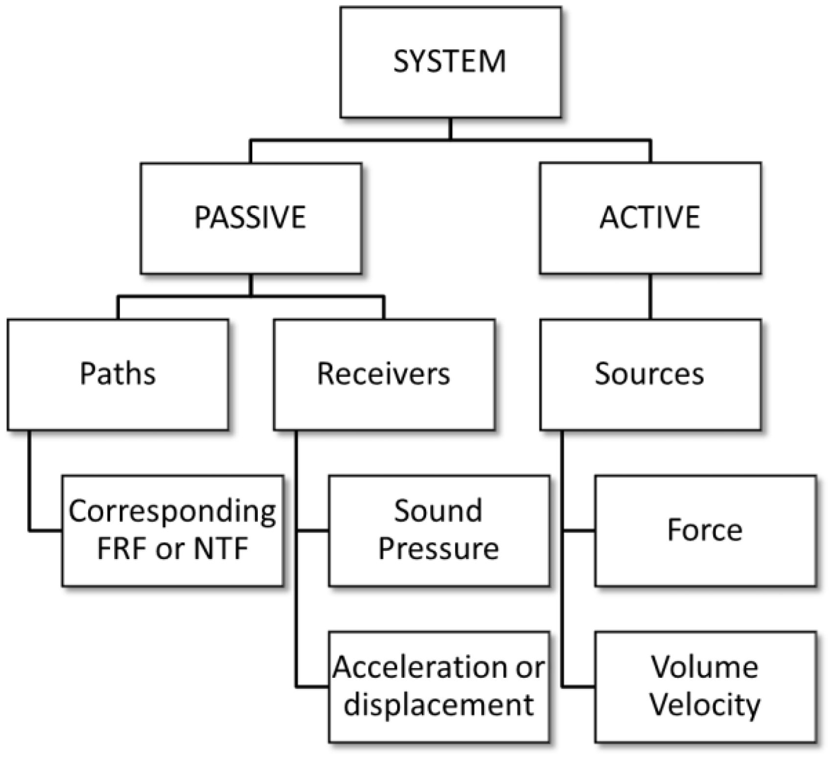

Traditionally, NVH problems have been analyzed using the modal analysis approach.^1–5 However, modal analysis may not be as effective when there are too many modes contributing in similar amounts to the problem. This is due to the fact that it is not convenient to trace and change all modes in order to solve the problem. Consequently, alternative methods such as TPA have been studied to solve the NVH problems in an effective manner.

TPA mainly involves three main subtopics which are related to each other, as shown in Figure 2. In cases when the goal is to determine the operational forces acting on the structure, especially for the purpose of source localization or structural health monitoring, operational force identification (OFI) subtopic of TPA can be used. If one is just interested in the operational response of any point, operational response prediction (ORP) subtopic of TPA can be applied after OFI. This topic can be implemented for design optimization, component selection, or condition monitoring purposes. Final subtopic of TPA is called path contribution which actually reveals the problematic path or source. In this topic, the dominant paths and the contribution of each path to the response are determined in order to solve the NVH problem.

Figure 2.

Subtopics of transfer path analysis.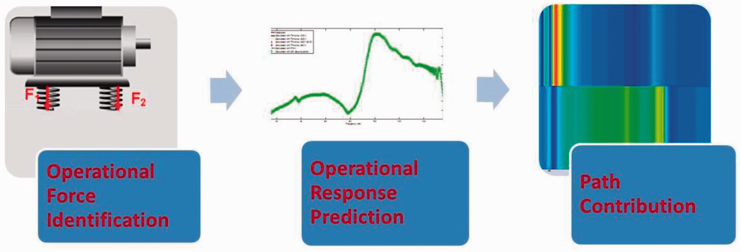

After initial development in the early 90 s, TPA has been extensively used as an effective tool in solving NVH problems by using experimental data, especially in the automotive industry. However, conventional TPA methods require great effort and measurement time. As far as the importance of simplicity and speed in the industrial applications are considered, many researches have been conducted for simpler and faster TPA methods as presented in literature.^6–12 In some methods, such as fast TPA and multilevel TPA, the goal is to reduce the component loads to equivalent virtual locations and some studies aim at reducing the number of transfer functions.¹³ In the operational TPA (OTPA) method, only operational data at the path references and targets are required but no transfer functions are needed. Parametric models have recently been applied to identify the operational forces. This method is referred to as operational path analysis with exogenous inputs (OPAX).^8–11 Due to some critical limitations, such as potential cross-coupling, ill-conditioning problems and quality of prediction, further studies have been ongoing to find a combination of fast, easy, and reliable methods.

In this study, ORP is discussed especially for rigidly linked vibrating structures since real and complex structures have many coupled rigid links. Applicability and accuracy of direct inversion method, which is more practical and time efficient, is presented. Besides, the importance of the cross-coupling terms and measurement errors are discussed. This paper is organized as follows: Section ‘Matrix inversion methods’ focuses on the matrix inversion techniques such as Moore–Penrose pseudo inversion, direct inversion, and some theoretical considerations such as over-determination of accelerance matrix and the effect of cross-coupling terms. Section ‘Experimental validation of the matrix inversion methods’ presents case studies conducted in accordance with the developed methodologies and demonstration of the measurement errors such as mass loading and noise. Finally, the paper is concluded with a summary and conclusion in Section ‘Summary and conclusions’.

Matrix inversion methods

The first step of ORP is identifying the operational internal forces acting on the transmission paths between active and passive parts of the system. The operational forces at the transmission paths can be directly measured or indirectly calculated. Although it seems reasonable to measure the forces in a direct way by means of force transducers, it is almost impossible and totally impractical for complex structures since special transducers have to be constructed in order to split the forces in three orthogonal components without affecting the overall dynamics of the structure. Thus, in most of the existing studies, the operational forces are predicted by using operational response measurements. These indirect procedures involve mount stiffness method^14,15 and matrix inversion methods.^16,17 When the transfer paths include rigid connections or the mounts are very stiff compared to the receiver, the dynamic stiffness method cannot be implemented since the relative response across the mount becomes too small.¹⁵ Since rigid connections are considered, the matrix inversion method is the point of interest.

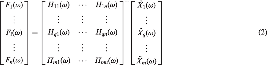
For the structures with rigid connections the matrix inversion method must be used. This method involves direct or reciprocal measurement of transfer functions, frequency response functions (FRFs), and operational response measurements. Then, accelerance matrix is constituted by placing these FRFs into the corresponding column (path number) and row (sensor number). Operational internal force acting at each path is calculated by multiplying the measured operational responses with the inverse of accelerance matrix, as

{F (ω)} = [H (ω)]^{- 1} {\overset{··}{X} (ω)}

(1)

Moore–Penrose pseudo inversion

Moore–Penrose pseudo inversion method identifies the internal forces by isolating each path. In other words, FRFs are measured between the response and source points, respectively, such that the corresponding path remains in place, while all other path connections are disassembled from the receiving subsystem of interest. Since the energy flows through only the remaining path during FRF measurements, the cross-coupling effects are assumed as negligible. Additionally, the number of response points (m) to be measured should be larger than the number of forces to be identified or so-called paths (n). As a rule of thumb, m ≥ 2 n is usually taken.^6,11,18 Thus, the system will be over-determined when using larger number of responses than the forces to be identified and making a least-squared error solution. Using additional information can help to reduce the measurement errors, which especially occur due to noise.^19,20

Due to applying over-determination to reduce the measurement errors, the accelerance matrix becomes rectangular resulting in a system of linear equations which lack a unique solution. Thus, some matrix decomposition and least-squared error solution should be employed in accordance with the explained strategies. Moore–Penrose pseudo inversion can be used to compute a least-squared solution to a system of linear equations, as²¹

[F_{1} (ω) : F_{i} (ω) : F_{n} (ω)] = [H_{11} (ω) \dots H_{1 n} (ω) : : : H_{q 1} (ω) \dots H_{qn} (ω) : : : H_{m 1} (ω) \dots H_{mn} (ω)]^{+} [{\overset{··}{X}}_{1} (ω) : {\overset{··}{X}}_{q} (ω) : {\overset{··}{X}}_{m} (ω)]

(2)

Herein

H_{mi} (ω)

is the frequency response function (FRF-accelerance) measured between the sensor point m and the applied force at the interface connection of transfer path, i where i = 1, … , n (number of paths). “+” indicates the Moore–Penrose pseudo inversion and

{\overset{··}{X}}_{j} (ω)

is the operational response (acceleration) measured at sensor number j where j = 1, … , m (number of sensors)

Moore–Penrose pseudo inverse of accelerance matrix, H is given by

[H (ω)]^{+} = ([H (ω)]^{H} [H (ω)])^{- 1} [H (ω)]^{H}

(3)

where H indicates the Hermitian transpose (complex conjugate transpose). Hereby, the least-squares solution of equation (2) becomes

{F (ω)} = ([H (ω)]^{H} [H (ω)])^{- 1} [H (ω)]^{H} {\overset{··}{X} (ω)}

(4)

It should be noted that the solution should be worked out for each frequency, separately.

Condition number, which is simply the ratio of the largest singular value to the smallest one, is essential for the ill-conditioning problem. High condition number indicates that the FRF matrix is ill-conditioned and the solution may not be unique. Over-determination can reduce the condition number of the accelerance matrix at high frequencies, but it is ineffective at low frequencies where only a few modes contribute to the response. Linear dependency of the columns is also an important item in matrix inversion. If many modes contribute to the responses, the columns of the accelerance matrix will be independent and hence, this will result in low condition number.^19,22,23 Additionally, insignificant singular values should be rejected according to a threshold value to improve the conditioning of the accelerance matrix. A threshold can be defined according to FRF or operational response measurement errors which are basically based on the coherence value.^7,24 By applying singular value decomposition (SVD), the singular values for each frequency are revealed and hence, the smallest insignificant singular value of the accelerance matrix is set to “zero” according to the defined criterion. In this regard, the SVD method can also be referred to as a regularization method.²⁵

Although the measurement errors are eliminated as much as possible by making the accelerance matrix over-determined, the main drawback of pseudo inversion method is the need to perform a large number of FRF measurements after removing the source, which results in considerable time consumption. Since the system is required to be disassembled during the FRF measurements, the boundary conditions are not the same anymore and disassembling the structures cannot be always possible.^9,10,26

Direct inversion method including cross-coupling terms

The operational response of any point depends on corresponding transfer function and the force acting at that point if there is only one path. However, if more than one source or path is present, the cross-coupling terms should be taken into consideration. Cross-coupling means that the response at a particular point depends not only on the force acting at that point but also on other internal forces.⁶ Cross-coupling effects are considered by means of including all FRFs between the path inputs at the active side;

{\overset{··}{X}}_{1} = F_{1} H_{11} + F_{2} H_{12} + \dots + F_{n} H_{1 n}

(5)

where n represents the number of path inputs or internal forces. As can be seen in equation (5), a high response at any point does not imply that the force acting at that location is the only contributor. Thus, unconsidered cross-coupling terms lead to a false identification of operational response at the target point. Biermayer et al.¹³ state in their study that the error can be up to 10 dB if the cross-coupling terms are not adequately included.

In this approach, force identification process is applied at the active (source) side, whereas in pseudo inversion method, it is based on measurements at the passive (receiver) side. Thus, operational measurements are performed at the interface connections of the path inputs and FRFs are measured between the path inputs without disassembling them in order to consider the cross-couplings.

A square accelerance matrix, n x n, is created since the number of forces and responses are equal to each other. Thus, internal forces can be identified in matrix notation by applying ordinary matrix inversion as

{F_{i} (ω)} = [H_{ji} (ω)]^{- 1} {{\overset{··}{X}}_{i} (ω)}

(6)

where i = j denotes the number of paths and forces.

Once the operational forces acting on each path are calculated, the operational response at the point of interest or target k and the contribution of each path to that point can be predicted assuming that the system is linear and time-invariant. Partial contribution of each path to the operational response at the target can be identified by multiplying the calculated internal force acting at the path and measured FRF between the target and the source location. By adding up these partial contributions, the operational response at the target is calculated as

{\overset{··}{X}}_{k} (ω) = \sum_{i = 1}^{n} {\overset{··}{X}}_{ki} (ω) = \sum_{i = 1}^{n} F_{i} (ω) H_{ki} (ω)

(7)

In addition to the calculated operational response, the dominant transfer paths are identified. Using equation (7) the main causes of high contributions of a dominant path can be determined such as high transfer function, high force, high point mobility etc. Then, some remedial measures or corrections can be taken by means of reducing transfer functions, retuning attachment mount rates, or increasing local stiffness.

Experimental validation of the matrix inversion methods

In accordance with the statements of operational response identification methodologies, mentioned in previous sections, a rigidly linked setup was created in order to predict the operational response at the defined target by applying the matrix inversion method. The setup consists of two rigidly linked subsystems. The lower beam, clamped at one end, is the active part of the system, while the upper beam is the passive one. The setup is shown in Figure 3, and the corresponding material and physical properties are presented in Table 1. The validation is conducted both experimentally and numerically.

Figure 3.

Rigidly linked setup.

Table 1.

Material and physical properties of the setup.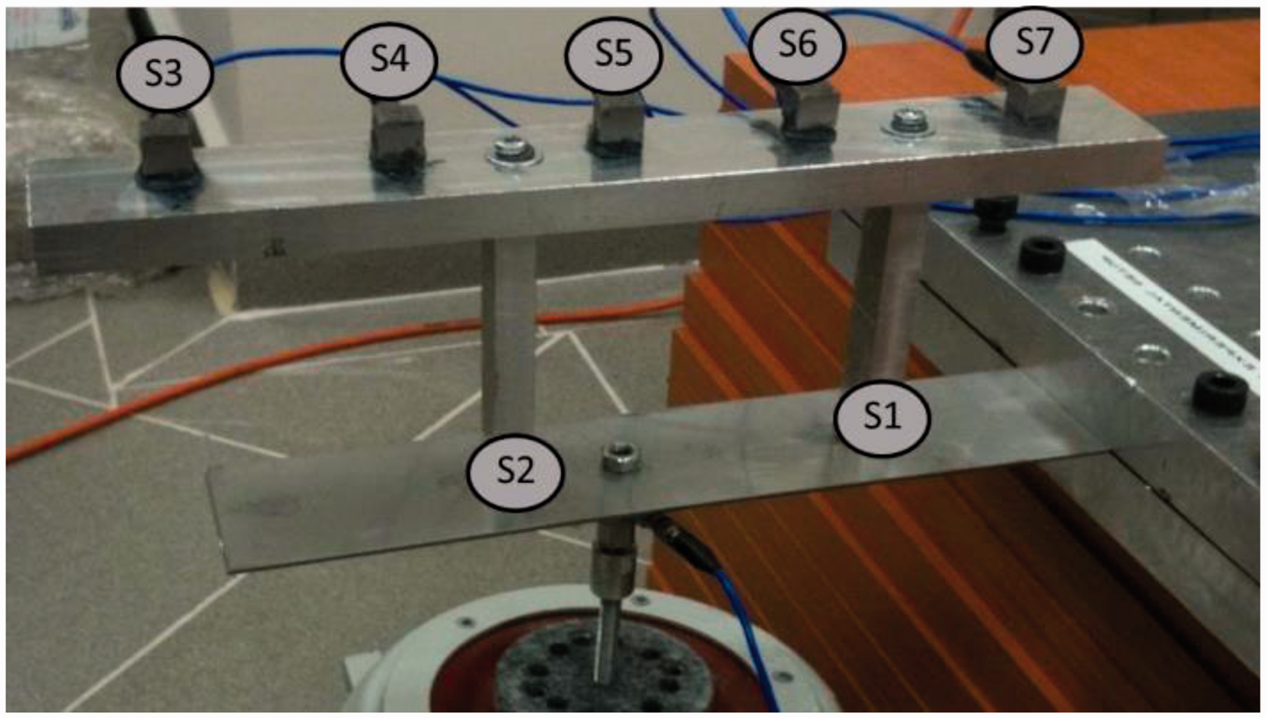

Properties	Upper beam	Lower beam	Links
Material	Steel	Steel	Aluminum
Young’s modulus (GPa)	200	200	78
Density (kg/m³)	8095	8095	2700
Length (mm)	265	230	86
Width (mm)	40	50	20
Thickness (mm)	15	1.5	10

Experimental case study

Experimental study is composed of three parts. First, the operational responses (acceleration) are measured by accelerometers. A modal shaker is used for excitations representing the operating source and connected to the structure through a force transducer used for measuring operational force for purposes of comparison. The operational responses should be measured as complex quantities with magnitude and phase information. Therefore, they can be derived for each frequency by using auto- and cross-spectra as

a_{i} = \sqrt{G_{ii}} e^{- j ∠ G_{i 1}}

(8)

where G_ii is the auto-spectrum of the response at point i, which gives the amplitude, and G_i₁ is the cross-spectrum between the reference position1 and point i, which forms the complex part. It should be noted that equation (8) should only be used if the coherence function between a₁ and a_i is about one and the reference position should be one of the points where the operation response is measured.^19,27

Second part is to measure the accelerances of the structure via modal shaker from source location to the target locations. H1 is taken into account as the transfer function and the frequency range of interest are selected as 0–300 Hz. Finally, the third part is composed of data processing, implementing the mentioned methodologies and presenting the results as well as comparing the calculated operational response of the target with the measured one. This comparison serves as an indicator of the quality of the methods.

Although there is one operational force acting on the active substructure, there should be vibrational energy flowing through the links resulting in internal forces. It is actually difficult to realize a pure one-dimensional excitation at the level of links because unmeasured moments and lateral forces may be introduced, but at the same time, moments and rotations are neglected in TPA since they are very hard to measure.¹⁸ Nevertheless, the aim of this study is to estimate the internal forces acting in the vertical direction and thus, the operational responses, assuming that the system is time-invariant and linear. The total estimated force was simply taken as the sum of the internal forces.

The first study was conducted in relation to Moore–Penrose pseudo inversion method as explained in Section ‘Moore–Penrose pseudo inversion’. After the operational measurements were conducted at the sensor points, the system was disassembled at each link or path respectively and FRFs were measured through each path between the sensor points and the source point by using an impact hammer. Accelerance matrix was constituted by importing FRFs to the corresponding columns and rows which represent the paths and the sensor numbers, respectively. Operational response and FRFs were measured at five sensors located at the passive side, as shown in Figure 4. Four of these were taken into account in order to make the system over-determined since the number of sensors should be at least equal to the number of forces to be identified, as a rule of thumb. The fifth one was selected as the point of interest, so-called target, where the operational response was aimed to be predicted. Thus, the measured transfer functions and operational response corresponding to the target were not included in the force identification algorithm. Nevertheless, the operational response at the target was used for comparison purposes.

Figure 4.

FRF measurements for pseudo inversion method.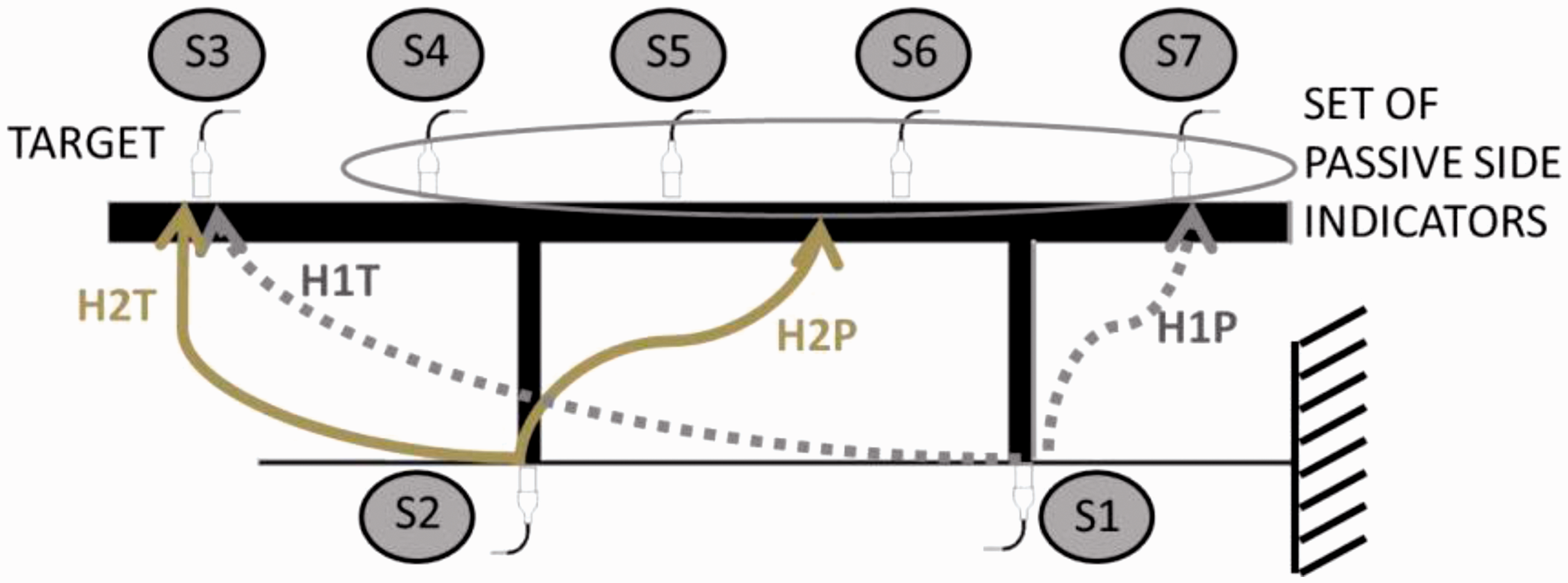

Following the constitution of the accelerance matrix, SVD was applied to improve the condition number of the matrix and then the modified matrix was inverted by implementing the Moore–Penrose pseudo inversion in order to calculate the operational force. After identifying the operational force, the operational response at the selected point of interest was predicted by implementing equation (7). The calculated operational responses at the sensor point 3 and 4 are presented in Figure 5(b) (d), whereas the FRFs measured with respect to each path are presented in Figure 5(a) and (c).

Figure 5.

(a) FRFs measured at S3; (b) Operational response at S3; (c) FRFs measured at S4; (d) Operational response at S4.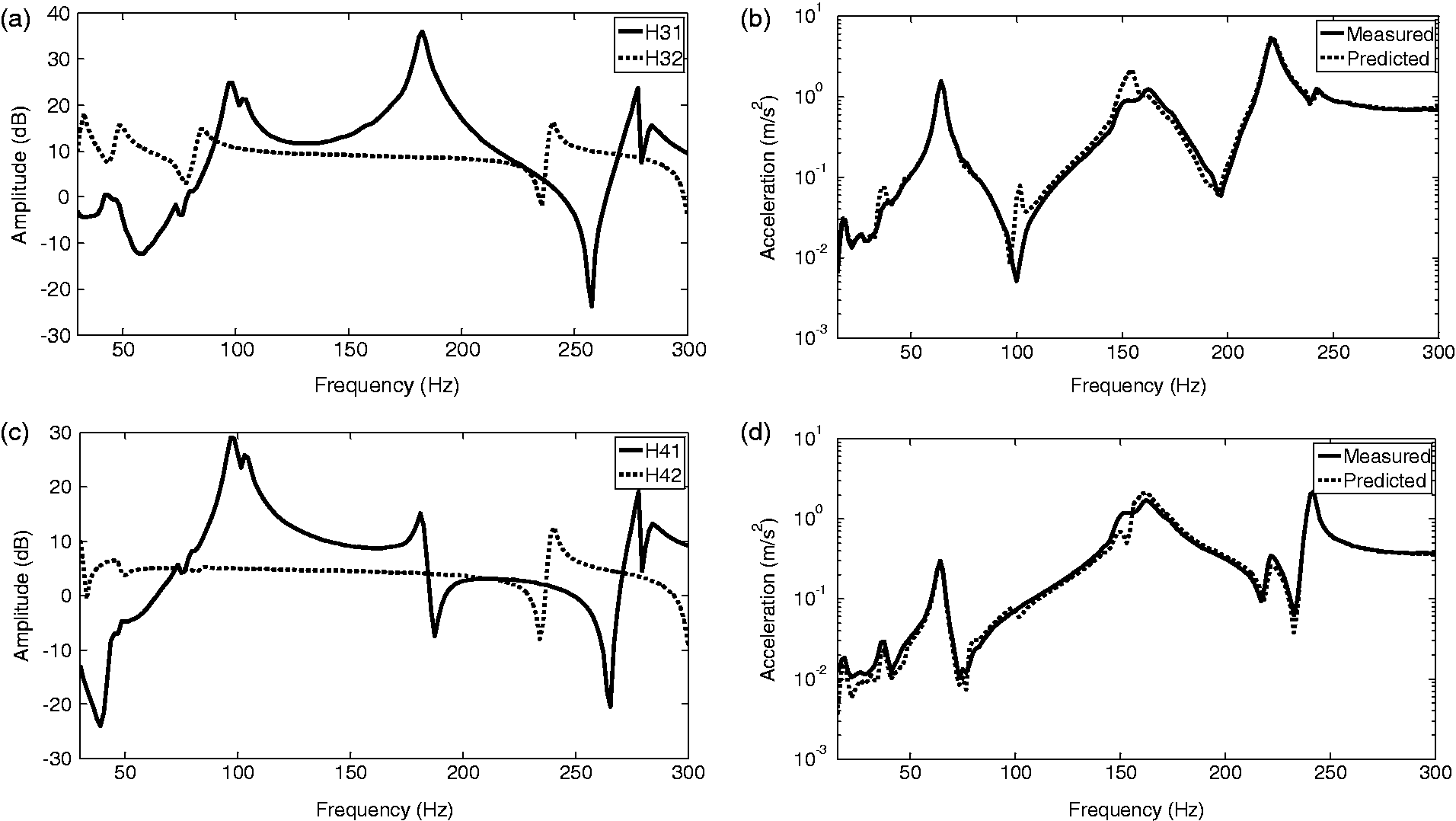

The FRFs indicate that the structure does not exhibit strong modal correlation through the paths, which results in linear independency at the corresponding columns of the accelerance matrix, as mentioned in Section ‘Matrix inversion methods’. Therefore, predicted responses at the targets almost match with the measured ones. However, there are still some discrepancies between the predicted and measured responses. For point S3, it is clearly observed that the variation occurs especially at 100 Hz and 150 Hz range. Figure 6 shows the condition number of the accelerance matrix as a function of frequency. This actually confirms that the condition number is a good quality indicator of the identification based on the matrix inversion method since one can observe noticeably large condition numbers within the 100–150 Hz region. It is also clearly noted that over-determination reduces the condition number of the accelerance matrix at higher frequencies, but it is ineffective at lower frequencies where only a few modes contribute to the response, as discussed in literature.^8,19,22,23 However, at higher frequencies, where the modal overlap is greater, over-determination gives significant reduction in condition numbers. Since measurement errors occur in any FRF measurement, these errors will be amplified by the inversion of the accelerance matrix, especially at frequencies where the condition number is high and thus, the condition numbers serve as the parameters influencing the error amplification. The considerations stated in this paper improve the conditioning of the matrix and thus reduce the effect of the introduced measurement errors but cannot exactly compensate for them.

Figure 6.

Condition number of the accelerance matrix.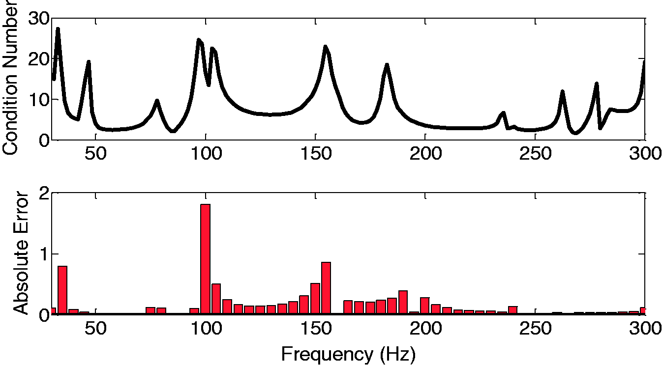

The direct inversion method described in Section ‘Direct inversion method including cross-coupling terms’was also applied for the same experimental setup in order to determine its effectiveness. The schematic representation of the setup and measurements are illustrated in Figure 7. Operational responses are measured at S1 and S2 located at the path inputs, while the operational responses at the target locations were just measured for comparison purposes. In the second step, FRFs were measured between the path inputs and the targets at the passive side without disassembling the setup.

Figure 7.

(a) Operational response measurement; (b) FRF Measurements for direct inversion method.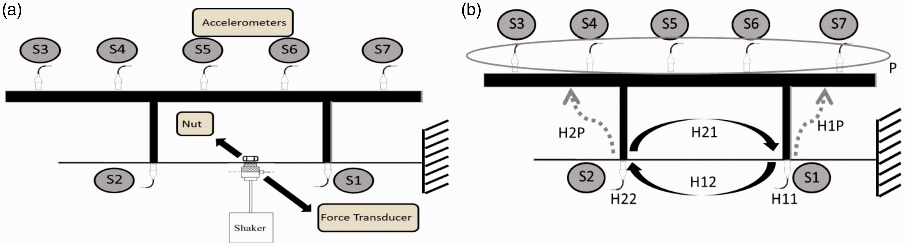

By implementing the direct inversion method along with the cross-coupling terms, the operational responses at the targets were identified. The points located at the active side of the structure were the targets where the response is to be predicted. As shown in Figure 8, the direct inversion method captured the spectral character of the measured response with slight magnitude differences and it can be stated that there is an acceptable correlation between the measured and predicted results.

Figure 8.

Operational responses: (a) at S3; (b) at S4; (c) at S5; (d) at S6.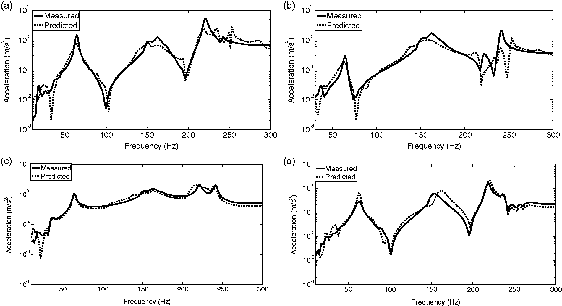

In addition to the ORP, the question is now to determine the path dominating the response at a particular frequency by these methods. For that purpose, path contribution plots (PCP) are generated. PCP shows the amplitude of the partial contributions for the paths as a function of frequency. Since at 220 Hz and 240 Hz, the response of point S3 has the highest value over the entire frequency range, the PCPs are exhibited between 200 and 300 Hz in Figure 9. As shown in Figure 9, path 2 is determined as the dominant path on the response at 220 Hz and 240 Hz, and both methods have a good agreement on the path contribution with corresponding frequencies.

Figure 9.

Path contribution plots for S3: (a) direct inversion method; (b) pseudo inversion method.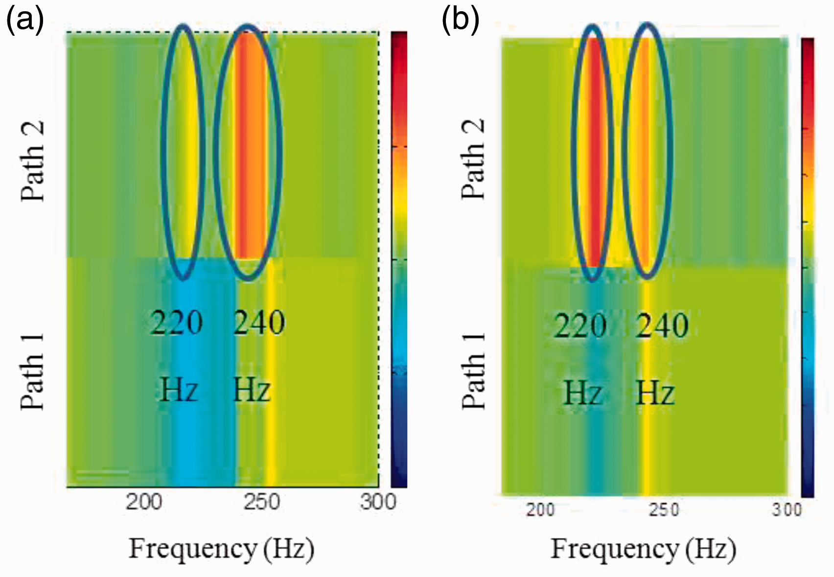

In the operational response predicted by the direct inversion method, there are some unavoidable discrepancies which can occur due to the combination of some assumptions and measurement errors. In this study, the rotations, moments, and lateral forces are neglected as in many experimental analyses.¹⁸ Additionally, it is assumed that the sum of energy flowing through all paths to the target is always equal to the total energy as measured at the target location. However, there may be transmission loss through the active subsystem.

In addition to the linear energy flow assumption, there are also measurement errors in the experimental studies. The testing process is prone to errors introduced by various factors. Among these, one of the factors is the mass loading effect of the force transducer. As illustrated in Figure 7, a modal shaker is used for the FRF measurements and connected to the structure through a force transducer by means of a screw and nut. Since this transducer is mounted on the structure, the dynamic of the setup is changed and consequently, the measured FRF contains errors, as discussed in literature.^28–30 Besides, excessive tightening of the nut can result in additional inertia mass. This mass loading effect can be significant since the setup is a light-weighted structure. Another factor is the alignment of the shaker. Misalignment is an important item of concern which can cause distortion of the measured data.³¹ Moreover, measured data are usually contaminated with other adverse effects such as noise.

Numerical case study

A numerical case study is presented to verify the method as well as to demonstrate the effects of mass loading and noise on the experimental results of the ORP method. A finite element model (FEM) of the experimental setup is built to perform the numerical study (see Figure 10). The structure is excited at the lower beam by using the force spectral data obtained from the experimental study. The energy created by the excitation force propagates through the links to the upper beam. Thus, internal forces are introduced at the links and identified by applying both methods mentioned in Section ‘Matrix inversion methods’. However, numerical study conducted in accordance with direct inversion method will be presented for sake of brevity. Accelerance matrix, a size of 2 × 2, is composed of transfer functions measured at the points S1, S2 and also between each other for the purpose of including the cross-coupling effects. Operational responses at S1 and S2 are used in identifying the internal forces with the accelerance matrix, whereas the others are employed for comparison purposes. Thus, operational responses at the points of interest on the upper beam are predicted and compared with the actual one.

Figure 10.

Numerical model.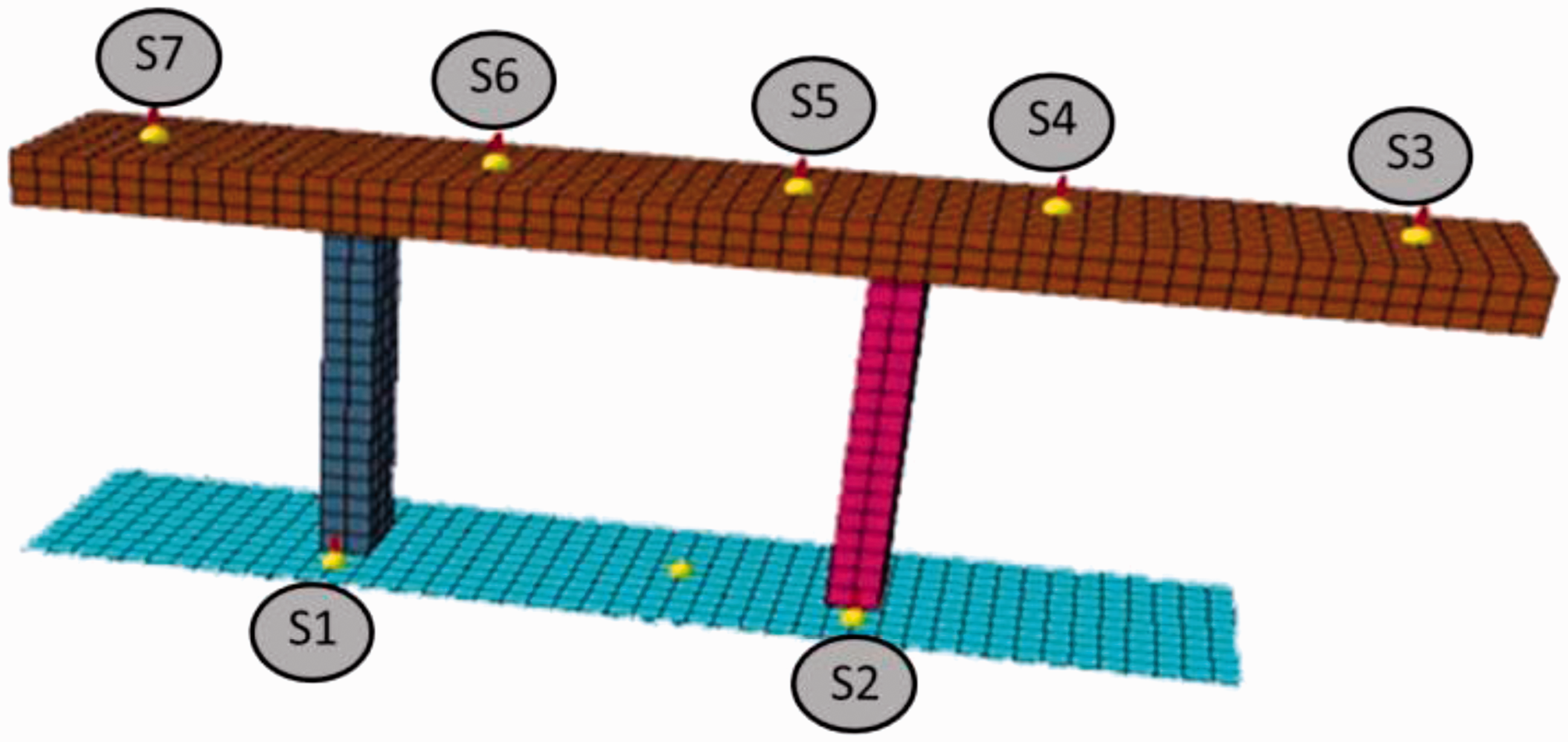

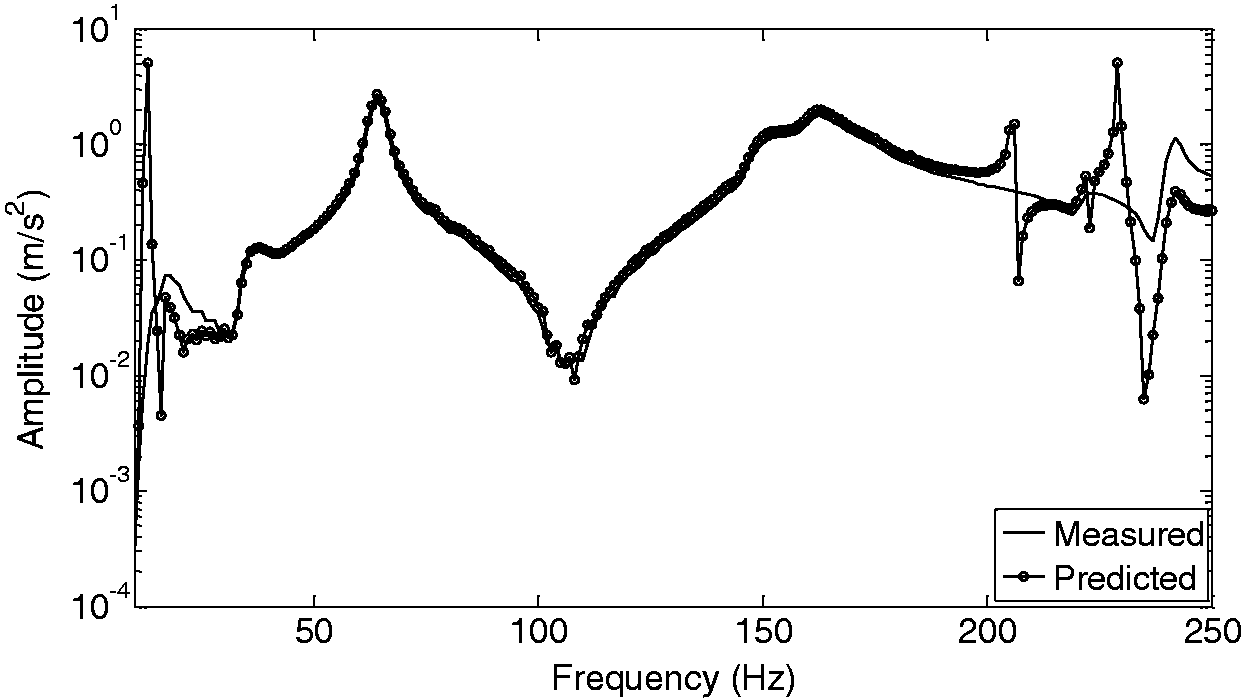
The predicted and actual numerical responses of S3 are shown in Figure 11. As noted the predicted response fits well with the actual one. The resonance frequencies are exactly the same while the amplitudes differ slightly. The internal operational forces are also determined without including cross-coupling terms. In other words, each internal force acting on the link is identified by using corresponding path input and its point transfer function. From the figure, it can be clearly observed that the prediction without including cross-coupling terms increases the overall error with about a rate of 10%–12% in the frequency band. Note that, a similar behavior is observed for the other measurement locations (e.g. S4, S5, S6, and S7).

Figure 11.

Predicted operational response of S3.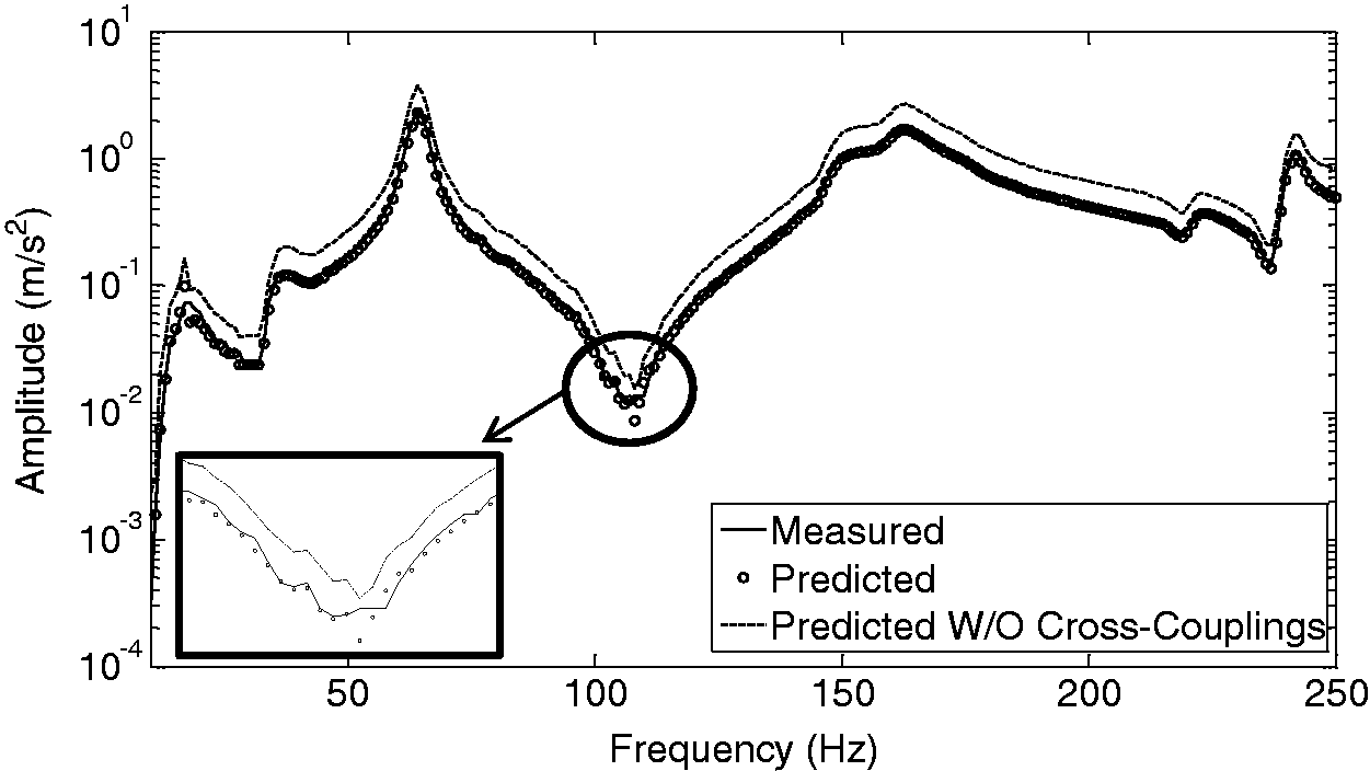

The comparison of measured and predicted responses can be accomplished by using a metric developed in previous validation studies.^32,33 This metric is based on the variance of the calculated and measured values. Variance, $σ^{2}$ , is a measure of variability involving deviations from the mean and gives the extent of concentration around the mean value.³⁴ The change of variance with frequency can be defined by the power spectral density (PSD), $S_{xx}$ which gives the power of the signal as a function of frequency.

\frac{\partial σ^{2} (ω)}{\partial ω} = S_{xx} (ω)

(9)

Hence, the variance can be expressed as a function of frequency range

σ^{2} (f_{1}, f_{2}) = \int_{f_{1}}^{f_{2}} S_{xx} (ω) d ω

(10)

The variance shown in equation (10) can also be described as the cumulative absolute variance which is the contribution of frequency components within a frequency range to the total variance.³⁵ The accuracy of the method is determined by utilizing the square root of the variance, σ. For both experimental and numerical studies, the ratio of σ between the measured and calculated responses with applied methods is tabulated within a number of bandwidths in Table 2. The value of such metric highlights the correlation level between the measured and calculated results. The unity (1) value indicates a perfect match and values closer to unity are accepted as satisfactory.

Table 2.

Comparison of measured and calculated responses.

Applied methods	$σ_{calculated} / σ_{measured}$
Applied methods	0–50 Hz	50–100 Hz	100–200 Hz	200–300 Hz	0–300 Hz
Pseudo inversion
Experimental	1	0.80	1.03	0.85	0.91
Numerical	1	1	1.13	1.19	0.99
Direct inversion
Experimental	1.12	1.63	0.37	0.70	1.37
Numerical	0.99	0.90	0.87	1.15	1.07

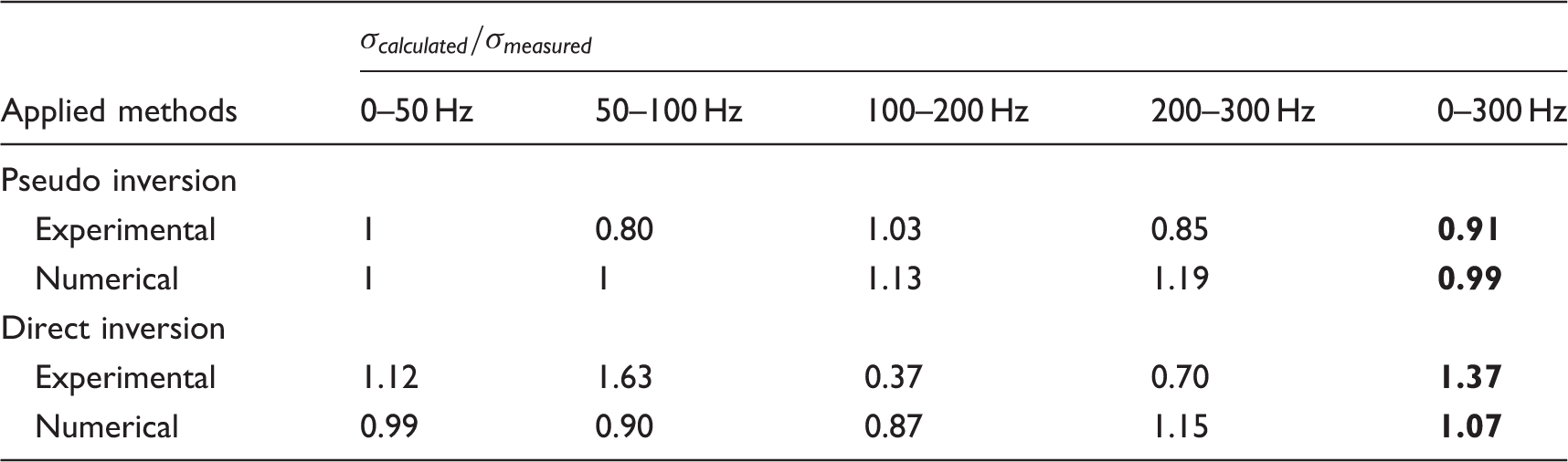
According to Table 2, the pseudo inversion method reveals a bit more accurate result than the direct inversion method does over the entire 0–300 Hz range. This is due to the fact that since the active side is separated from the passive side while determining the transfer functions, the cross-coupling effects are prevented.

As shown in the results, in the numerical study the predicted response matches with the actual one considerably well compared to the experimental study. The difference between the numerical and experimental results is assumed to occur due to combination of the FRF measurement errors and energy flow assumption, as explained in the previous section. These errors are magnified by the inversion of the accelerance matrix. Since real measurements are never made under perfect conditions, further simulations are focused on the measurement errors and applied to identify the significance of these effects on the operational response identification. These adverse effects are composed of mass loadings due to the force transducer and shaker connections and the existing noise during the FRF measurements.

Demonstration of mass loading effects on the ORP

The mass loading effects occur due to usually ignoring the force transducer and the shaker connections in the experimental studies, based on the assumption that they are negligible compared to those of the structure. Nevertheless, if the structure is light-weight, then these mass effects can be significant. Thus, in order to demonstrate the effect of mass loading on the ORPs, point mass is intentionally added to the shaker connection points at the path inputs during the numerical FRF analysis. After obtaining the FRF data altered by the additional mass loadings at the path inputs, the accelerance matrix is constituted and the direct inversion method is applied. As can be seen in Figure 12, the condition number of the accelerance matrix is increased at each frequency and thus, the error in response identification is expected to be larger compared to the ideal numerical result. The operational response of S3 is presented in Figure 13. It is observed that discrepancies occur especially between 200 and 250 Hz, as expected according to the condition number. As illustrated in Figure 13, mass loadings can affect the results to have discrepancies between 20 and 30 dB in magnitude and similar results in the experimental study are also observed at mentioned frequency range in Figure 8.

Figure 12.

Condition number of the accelerance matrix.

Figure 13.

Operational response of sensor point S3.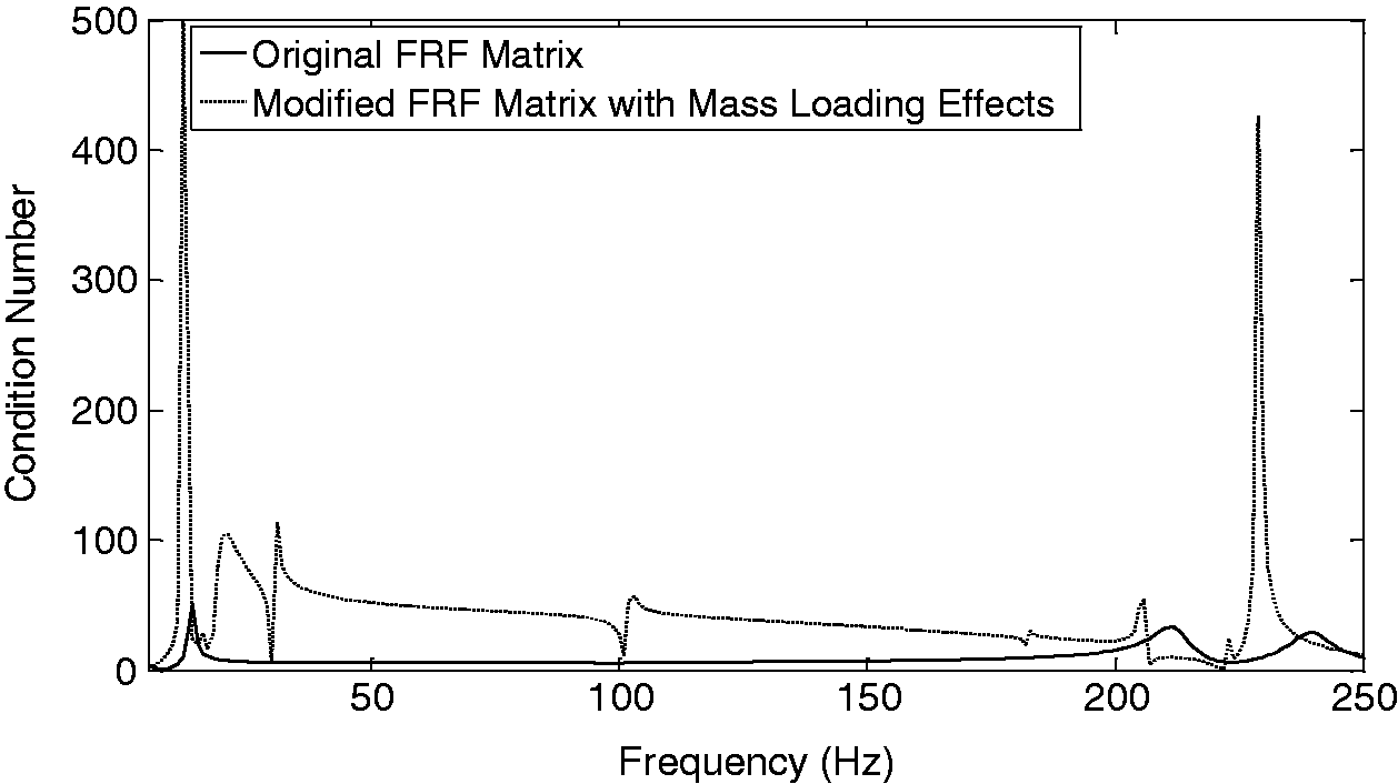

Demonstration of noise effects on the ORP

Along with the mass loading effects, FRFs measured in reality are also contaminated with other adverse effects such as noise. In any FRF measurement, noise exists at both the input and the output channels. For frequencies close to resonance and anti-resonances, the noise can be ignored since the vibration response is dominant. 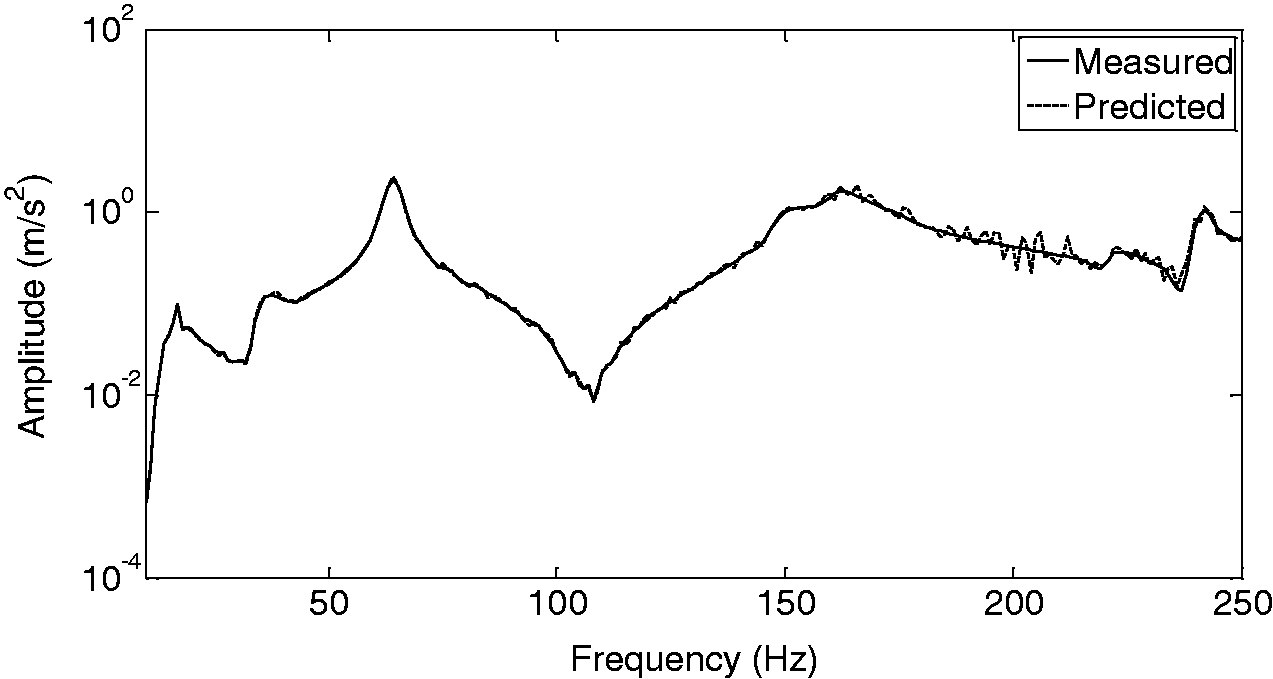However, for the other frequencies the noise can affect the FRF measurement from both ends.³⁶ In this study, further simulations are conducted to examine the result of the ORP in the case of noisy FRF data and consequently accelerance matrix. Thus, FRFs are numerically contaminated with additive white noise with a degree of contamination being 5% which results in ill-conditioned accelerance matrix, as illustrated in Figure 14. The procedures of the direct inversion method are applied again and the operational response of sensor S3 is predicted. The contamination of the FRF data with a degree of 5 % results in errors up to 6 dB as shown in Figure 15.

Figure 14.

Condition number of the accelerance matrix.

Figure 15.

Operational response of sensor point S3.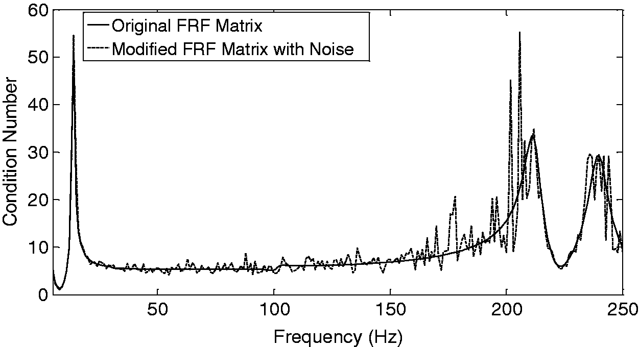

As can be observed in the numerical results, the experimental FRF measurements are prone to errors due to mass loadings and noise. These errors are almost unavoidable and result in larger condition numbers in accelerance matrix. Since the matrix is inverted, these errors are magnified at particular frequencies, as presented in Verheij^37,38 and thus, some discrepancies are determined at the operational response identified by the direct inversion method, as also seen in the experimental results. It can also be concluded that if the primary concern is the ORP and path contribution in terms of design optimization, condition monitoring, taking remedial measures, the direct inversion method can be implemented for this kind of structures since these methods require less effort and measurement time.

Summary and conclusions

In this study, the ORP methods based on matrix inversion methods were discussed with the numerical and experimental case studies. In the first part of the study, Moore–Penrose pseudo inversion method was presented. The measurements were conducted to constitute the accelerance matrix and operational response vector. Over-determination as well as SVD was also considered to improve the accelerance matrix to be inverted in order to identify the operational internal forces and then, predict the operational response at the point of interest. In this study, one dimensional and vertical operational force was applied and assumed to be the sum of vertical internal forces acting on the paths by ignoring the lateral forces and moments. As a consequence, pseudo inversion technique is proven to be reliable but its application requires huge effort as well as extensive time since the paths should be disassembled and a huge amount of FRF measurements are needed.

For the purpose of seeking faster and easier methods, the direct inversion method was presented and investigated in the second part of the study. Compared to pseudo inversion technique, this method is less time consuming, less challenging, and the real boundary conditions are represented in the FRF measurements since no disassembling is required. However, it has some limitations besides its advantages. All structures exhibit a certain amount of cross-coupling between the path inputs. Depending on the degree of cross-coupling, the identified response is unreliable. Since the system is not required to be disassembled, the cross-coupling effects should be considered. The operational response of the target was also predicted by implementing this method including the cross-couplings between the path inputs and a comparison metric based on the variance was used for determining the effectiveness with respect to defined frequency bandwidths. The results show that including cross-coupling terms improves the results with a rate of about 10–12% and the predicted responses agree quite closely both in character and magnitude with some discrepancies occurring due to the combination of assumptions and measurement errors. As demonstrated in the numerical study, the operation responses identified by the direct inversion method are prone to measurement errors such as mass loadings and noise. These errors are almost unavoidable and result in discrepancies at particular frequencies of the predicted response. As a consequence, the direct inversion method including cross-couplings can be implemented for this kind of rigidly linked structures if they are almost impossible to be disassembled and the primary concern is predicting the operational response as well as determining the dominant paths in terms of condition monitoring and design optimization.

Footnotes

Declaration of conflicting interests

The author(s) declared no potential conflicts of interest with respect to the research, authorship, and/or publication of this article.

Funding

The author(s) disclosed receipt of the following financial support for the research, authorship, and/or publication of this article: This work is supported by the Republic of Turkey Ministry of Science, Industry and Technology and Ford Otosan. The authors would like to thank Ford Otosan Vehicle NVH and Interior Quietness teams for their support on test plans, vehicle instrumentation, and data collection.

References

Heylen

Lammens

Sas

. Modal analysis theory and testing, Leuven, Belgium: Department of Mechanical Engineering, University of Leuven, 1997.

Ewins

. Modal testing: theory practice and application, Hertfordshire, UK: Research Studies Press Ltd, 2000.

Maia

NSJ

. Theoretical and experimental modal analysis, Somerser, UK: Research Studies Press Ltd, 1997.

Rodrigues

JFD

Lopes

Melo

. Experimental modal analysis of a synthetic composite femur. Exp Mech 2004; 44: 29–32.

Mohanty

Rixen

. Identifying mode shapes and modal frequencies by operational modal analysis in the presence of harmonic excitation. Exp Mech 2005; 45: 213–220.

Gajdatsy

Janssens

Desmet

. Application of the transmissibility concept in transfer path analysis. Mech Syst Signal Process 2010; 24: 1963–1976.

Janssens

MHA

Verheij

Thompson

. The use of an equivalent forces method for the experimental quantification of structural sound transmission in ships. J Sound Vib 1999; 226: 305–328.

Janssens

KGP

Van der Auweraer

. Operational path analysis: a critical review. ISMA 2008; 1: 3657–3673.

de Klerk

Ossipov

. Operational transfer path analysis: theory, guidelines and tire noise application. Mech Syst Signal Process 2010; 24: 1950–1962.

10.

De Sitter

Devriendt

Guillaume

. Operational transfer path analysis. Mech Syst Signal Process 2010; 24: 416–431.

11.

Janssens

Gajdatsy

Gielen

. OPAX: a new transfer path analysis method based on parametric load models. Mech Syst Signal Process 2011; 25: 1321–1338.

12.

Van der Auweraer H, Mas P, Dom S, et al. Transfer path analysis in the critical path of vehicle refinement: the role of fast, hybrid and operational path analysis. SAE Technical Paper 2007-01-2352, 2007.

13.

Biermayer W, Brandl F, Höldrich R, et al. Sound engineering based on source contributions and transfer path results. In: Journal of society of automative engineers of Japan annual congress, Austria, 2007.

14.

Multipath

. Sound transfer from resiliently mounted shipboard machinery, TNO-TH, Delft, Netherlands: Institute of Applied Physics, 1982.

15.

Plunt

. Finding and fixing vehicle NVH problems with transfer path analysis. Sound Vib 2005; 11: 12–16.

16.

Starkey

Merrill

. On the ill-conditioned nature of indirect force measurement techniques. Int J Analyt Exp Modal Anal 1989; 4: 103–108.

17.

Van der Linden P and Floetke H. Comparing inverse force identification and the mount stiffness force identification methods for noise contribution analysis. In: Proceedings of ISMA conference Leuven, Belgium, September 2004.

18.

Knapen

. Transfer path analysis related to booming, performed on a car, Eindhoven, Netherlands: Eindhoven University of Technology, 1999.

19.

Thite

Thompson

. The quantification of structure-borne transmission paths by inverse methods. Part 1: improved singular value rejection methods. J Sound Vib 2003; 264: 411–431.

20.

Renzi

Pézerat

Guyader

. Vibratory source identification by using the finite element model of a subdomain of a flexural beam. J Sound Vib 2013; 332: 545–562.

21.

Penrose

. A generalized inverse for matrices. Mathematical Proceedings of the Cambridge Philosophical Society, 51 1955, pp. 406–413.

22.

Thite

Thompson

. Selection of response measurement locations to improve inverse force determination. Appl Acoust 2006; 67: 797–818.

23.

Thite

. Inverse determination of structure-borne sound sources. Ph.D Thesis, Southampton, UK: University of Southampton, 2003.

24.

Janssens

MHA

Verheij

Loyau

. Experimental example of the pseudo-forces method used in characterisation of a structure-borne sound source. Appl Acoust 2002; 63: 9–34.

25.

Uhl

. The inverse identification problem and its technical application. Arch Appl Mech 2007; 77: 325–337.

26.

Mas P, Sas P and Wyckaert K. Indirect force identification based upon impedance matrix inversion: a study on statistical and deterministical accuracy. In: Proceedings of 19th ISMA conference 1994, Leuven, Belgium, 12–14 September, 1994.

27.

Janssens

MHA

Verheij

. A pseudo-forces methodology to be used in characterization of structure-borne sound sources. Appl Acoust 2000; 61: 285–308.

28.

Cakar

Sanliturk

. Elimination of transducer mass loading effects from frequency response functions. Mech Syst Signal Process 2005; 19: 87–104.

29.

Ren

Wang

. Elimination of transducer mass loading effects in shaker modal testing. Mech Syst Signal Process 2013; 38: 265–275.

30.

Dossing O. Prediction of transducer mass-loading effects and identification of dynamic mass. In: Proceedings of 9th international modal analysis conference, Florence, Italy, 15–18 April 1991, pp.306–312. Bethel, CT, USA: Society for Experimental Mechanics, Inc.

31.

Peres MA, Bono RW and Avitabile P. Effects of shaker, stinger and transducer mounting on the measured frequency response functions. In: Proceedings of ISMA 2012 international conference on noise and vibration engineering, Leuven, Belgium, 17–19 September 2012, pp.1475–1489. Red Hook, NY, USA: Curran Associates, Inc.

32.

Melody JW and Neat GW. Integrated modeling methodology validation using the micro-precision interferometer testbed. In: Proceedings of the 35th IEEE conference on decision and control Kobe, 11–13 December 1996, Vol. 4, pp.4222–4227. Kobe, Japan: IEEE.

33.

Basdogan

Elias

Dekens

. Predicting the optical performance of the space interferometry mission using a modeling, testing, and validation methodology. Transac ASME J Vib Acoust 2007; 129: 148–157.

34.

Devore

. Probability and statistics for engineering and the sciences, 6th ed. USA: Thomson, Boston, MA.

35.

Kochanczyk MD, Bartsch TF, Taute KM, et al. Power spectral density integration analysis and its application to large bandwidth, high precision position measurements. In: Proceedings of SPIE on optical trapping and optical micromanipulation IX, International Society for Optics and Photonics, Bellingham, WA, 2012, p.8458.

36.

Z-F

. Modal analysis, Woburn, MA: Butterworth-Heinemann, 2001.

37.

Verheij

. Inverse and reciprocity methods for machinery noise source characterization and sound path quantification, Part 1: sources. Int J Acoust Vib 1997; 2: 11–20.

38.

Verheij

. Inverse and reciprocity methods for machinery noise source characterization and sound path quantification, Part 2: transmission paths. Int J Acoust Vib 1997; 2: 103–112.

Operational response prediction for rigidly linked structures via direct inversion method

Abstract

Keywords

Introduction

Matrix inversion methods

Moore–Penrose pseudo inversion

Direct inversion method including cross-coupling terms

Experimental validation of the matrix inversion methods

Experimental case study

Numerical case study

Demonstration of mass loading effects on the ORP

Demonstration of noise effects on the ORP

Summary and conclusions

Footnotes

Declaration of conflicting interests

Funding

References