Sage Journals: Discover world-class research

Abstract

Successful automation of a machining process system requires an effective and efficient tool condition monitoring system to ensure high productivity, products of desired dimensions, and long machine tool life. As such the component’s processing quality and increased system reliability will be guaranteed. This paper presents a classification of healthy and faulty conditions of the face milling tool by using the Naïve Bayes technique. A set of descriptive statistical parameters is extracted from the vibration signals. The decision tree technique is used to select significant features out of all statistical extracted features. The selected features are fed to the Naïve Bayes algorithm. The output of the algorithm is used to study and classify the milling tool condition and it is found that the Naïve Bayes model is able to give 96.9% classification accuracy. Also the performances of the different classifiers are compared. Based on the results obtained, the Naïve Bayes technique can be recommended for online monitoring and fault diagnosis of the face milling tool.

Keywords

Condition monitoring machine learning decision tree Naïve Bayes

Introduction

The monitoring of machining processes can represent economy and practicality by identifying tool wear, surface roughness, and anomalies during metal cutting operation. Traditional assessment of tool life using Taylor’s tool life equation does not provide sufficient information about the complete life cycle of the tool. In some situations, it may lead to an overestimation of tool life and in some situations to underestimation of tool life and this will lead to excessive replacements of the tool. As a consequence, precious time and scarce resources are wasted. Excessive wear and tool breakage are the main reasons for the downtime. The damaged cutting tool can increase its strain level and result in poor surface finish of the product. Production rate increases significantly by reducing the machine tool downtime. Tool condition monitoring (TCM) is extremely viable in reduction of cutting tool downtime. In a TCM system, cutting process data, such as vibration, current signal, sound energy, surface finish, cutting force, temperature, image processing, etc. are acquired with sensors such as accelerometer, acoustic emission (AE) sensor, charge coupled device (CCD) camera, dynamometer, surface profiler, current sensor, pyrometer, etc.¹ Signal processing methods are used to analyze the data and some salient features are then extracted from the acquired raw signals. These extracted and selected features are used to optimize the process using artificial intelligence techniques. Actual data from the experiment and predicted values are compared to assess the precision of the technique. Then, controlling the machining process is possible by feeding the optimized data to the servo mechanism and machine controller.²

TCM techniques include direct measurement and indirect measurement of tool wears. Direct measurement of cutting edge provides the most accurate information about physical deterioration of the cutting tool. Park and Ulsoy³ adopted direct measurement method by using optical sensing techniques with computer vision. LoCasto et al.⁴ used CCD camera for tool wear measurement. Ryabov et al.⁵ used laser displacement sensor for online measurement of tool geometry in the milling process. They evaluated tool geometry failure through intensity and displacement of laser beam simultaneously. The literature based on direct measurement shows that the system will not be able to measure flank wear of dimension less than 40 µm. This is one of the limitations in direct measurement of TCM systems. Direct measurement offers good accuracy in certain conditions only. During machining, the cutting fluid surrounds the tool, making online direct measurements difficult. Currently, indirect measurements are found more suitable for online process applications.

In an indirect measurement system, the machining process data, such as force, vibration, AE, current/power, temperature, etc. are acquired and relevant features are extracted. Feature selection and ultimately, fault classifications based on selected features can be done using artificial intelligent techniques. Kuljanic and Sortino⁶ proposed tool wear indicators, namely torque force distance (TFD) indicator and normalized cutting force (NCF) indicator. They concluded that TFD indicator is better than NCF, because there is no need to determine the unworn tool cutting force and it is enough to compute the mean cutting force and actual mean torque. Tansel et al.⁷ investigated the performance of a genetic tool monitor system with the measured cutting force in the micro end milling of POCO EDM-C3 soft electrode in order to identify faults during operation. This approach is very conservative to abolish fault alarms during the process and it performed very accurately within framed time in the micro end milling process. Jemielniak and Arrazola⁸ studied an application of the combination of AE and cutting force signals in micro milling operation. They observed that there was a stronger influence of tool wear on AE signals than on cutting force signals. Marinescu and Axinte⁹ carried out an experiment on determining the malfunctions of both the tool and workpiece (Inconel 718) using cutting force and AE signals in end milling. They reported for the first time on possibility of predicting defects on workpiece surfaces by using AE sensors and they also found efficient performance of the combined effects of AE and cutting force signals on tool wear measurement and workpiece surface integrity. Rene et al.¹⁰ extracted cutting force signals from the driver current signal obtained from servo driver directly to predict sensorless tool breakage in computer numerical control milling machines.

Tool–workpiece material structural vibrations contain relevant features of tool wear. Orhan et al.¹¹ investigated the tool wear in time and frequency domain analyses during end milling of AISI D3 cold work tool steel using vibration signals. They observed that there was no considerable increase in the vibration amplitude until a flank wear reached 160 µm, above which the vibration amplitude increased significantly. Hsueh and Yang¹² employed support vector machine (SVM) method for tool breakage monitoring system in face milling of 7075 Aluminum through spindle displacement signals. Experimental results have shown that this approach is reliable, highly sensitive, and robust in signal processing and also tool breakage monitoring can be implemented successfully. Elangovan et al.¹³ used principal component analysis and C4.5 algorithm for tool wear classification. They concluded that the decision tree (C4.5 algorithm) is a better method for feature selection as compared to the principal component analysis method. Jantunen¹⁴ presented signal analyses, diagnostic techniques, and summary of monitoring methods for tool wear in the drilling process. Researchers have often used the diagnostic tools such as fuzzy logic,¹⁵ neural networks,^16,17 adaptive neuro fuzzy inference system,¹⁸ etc. However Sokolowski¹⁹ noticed a poor classification of tool wear by fuzzy logic. Sugumaran et al.²⁰ used the decision tree technique for feature selection and proximal SVM for classification of faults in roller bearing. Painuli et al.²¹ analyzed the vibration data for tool health monitoring in turning using K-star algorithm. They concluded that the K-star algorithm is able to achieve 78% classification accuracy.

The aforementioned literature provides motivation to work on the TCM system with an efficient and effective intelligent technique. This study aims to use vibration signals of healthy and faulty conditions of a face milling cutter for condition monitoring. In order to extract useful information, descriptive statistical parameters such as standard error, kurtosis, mode, range, mean, and median are selected from raw signals using decision tree. The Naïve Bayes algorithm is used to classify different conditions of the tool using the selected features.

Experimental setup

Experiments were carried out using a universal milling machine with recommended machining parameters by tool producer (M/s Mitsubishi) such as depth of cut 0.5 mm, feed 0.067 mm/tooth, and cutting speed 75 m/min. A face milling cutter (6 Carbide inserts, Mitsubishi make: SEMT13T3AGSN- VP15TF) of 80 mm diameter and workpiece material of AISI H13 steel were used in this study. The experimental setup is shown in Figure 1.

Figure 1.

Experimental setup for tool condition monitoring.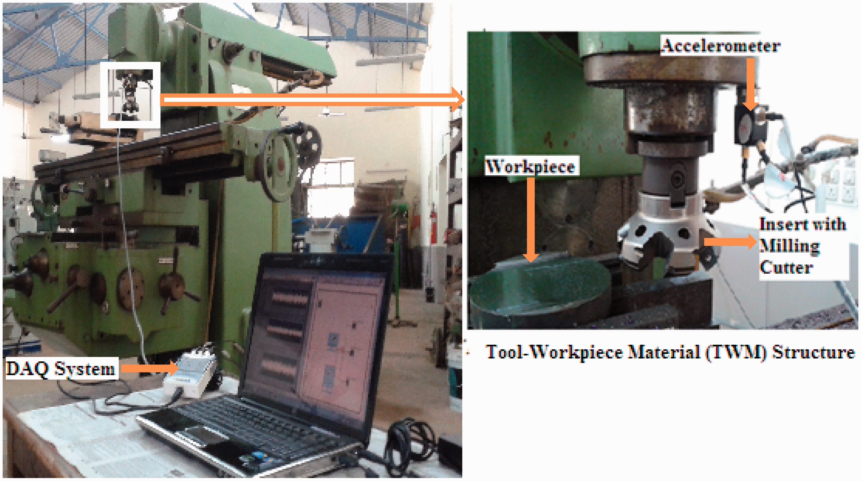

Experiments were conducted with four different conditions of the tool, out of which one is healthy and three are faulty conditions, namely

Chipping on the rake face (chipping);

Tip breakage (breakage);

Flank wear.

In the healthy condition of the tool, all six inserts are new/unworn inserts (Figure 2(a)), whereas in faulty condition among six inserts one is either chipping or breakage or flank wear (Figure 2(b) or (c) or (d)) have been considered for analysis. Vibration signals were acquired using triaxial piezoelectric accelerometer (YMC145A100, response frequency >15 kHz, measurement range ± 50 g, and sensitivity 106.3 mV/g) mounted on spindle housing. Data acquisition system NI DAQ 9234 (24-Bit, ± 5 V, 4 channel module) was used to acquire acceleration signals from the sensor; subsequently, analog signal was converted to digital by a DAQ system with sampling frequency of 25.6 kHz. These signals were processed using LabVIEW software and data were recorded on a computer.

Figure 2.

Different conditions of face milling tool insert. (a) Healthy, (b) chipping, (c) breakage, and (d) flank wear.

Figure 3.

Time series plots of (a) healthy, (b) chipping, (c) breakage, and (d) flank wear tool conditions.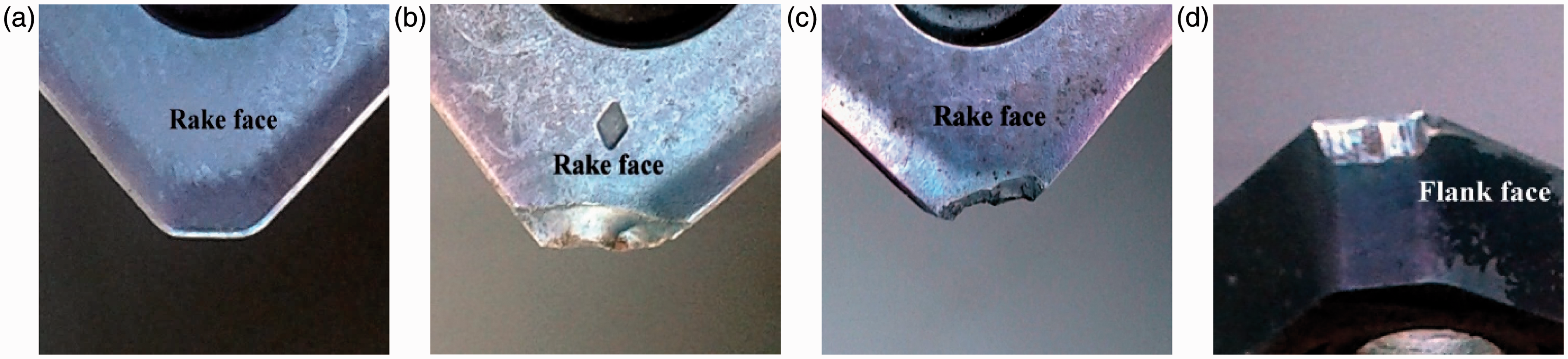

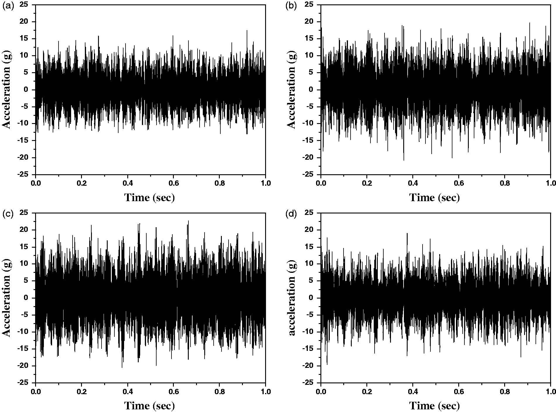
Rough machining was carried out with few passes to remove oxide layer and unevenness on the workpiece. The process was kept running for a few minutes to stabilize the machine, vibrating parts at initial stage. The vibration signals were acquired for healthy and different faulty conditions of the tool. A total of 160 samples were taken out of which 40 samples were for each condition of the tool with time interval of 1 s at sampling frequency of 25.6 kHz. Figure 3 shows the time series plots in feed direction for different conditions (healthy, chipping, breakage, and flank wear) of the milling tool.

Machine learning system

Machine learning is a scientific method to examine diagnostically the construction and study of algorithms that can learn from data. These algorithms build a model based on inputs and use that to make decisions or predictions, rather than following only explicitly programmed instructions. The flow chart of machine learning system for fault diagnosis of face milling cutter is as shown in Figure 4.

Figure 4.

Flowchart of machine learning system.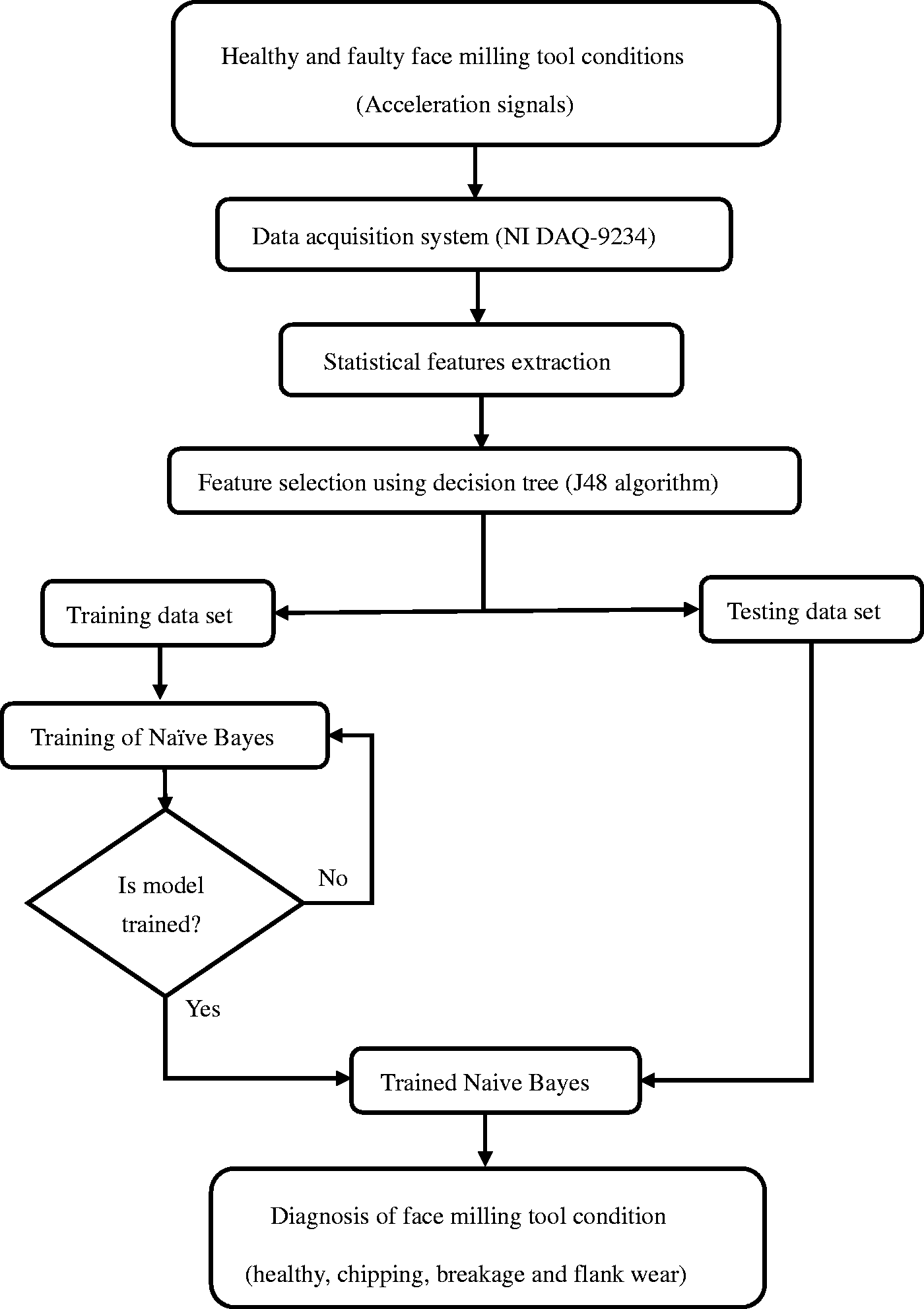

The experimental setup includes machine, sensor mounting, and DAQ system connection as described in “Experimental setup” section and further steps of the machine learning system will be discussed in forthcoming sections.

Feature extraction

The acquired vibration signals have different kinds of features which convey useful information about the raw signal. For example, statistical features, wavelet features, histogram features, etc. can be extracted from the acquired signals. Feature extraction is a process of extracting a set of new features from the raw signal through some functional mapping.²² Statistical features considered in the present study for analysis and the extracted features are discussed below.

Statistical features extraction

The parameters computed directly from the acquired time domain signals are called time domain features. Statistical features are one set of time domain features and significant ones in fault diagnosis of machine components/cutting tools. Here statistical features will be extracted for fault classification of face milling cutter. Statistical features such as skewness, mode, standard error, maximum, minimum, range, sum, mean, standard deviation, median, sample variance, and kurtosis are computed to serve as features. Brief descriptions about statistical parameters are displayed as follows.

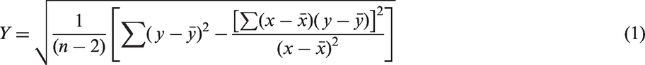
Standard error: Standard error is for an individual x in the regression, a measure of the amount of error in the estimation of y, “n” is the sample size, x and y are the sample means. It can be expressed as

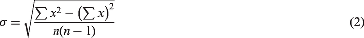
Y = \sqrt{\frac{1}{(n - 2)} [\sum (y - \bar{y}) 2 - \frac{[\sum (x - \bar{x}) (y - \bar{y})] 2}{(x - \bar{x}) 2}]}

(1)

Standard deviation: This is a measure of power content or effective energy of the signal. The standard deviation (σ) can be expressed as

σ = \sqrt{\frac{\sum x 2 - (\sum x) 2}{n (n - 1)}}

(2)

Sample variance: It is variance of the signal points and the following formula is used to compute sample variance

Sample Variance = σ 2 = \frac{\sum x 2 - (\sum x) 2}{n (n - 1)}

(3)

Kurtosis: Kurtosis represents the spikiness or the flatness of the signal. Its value varies with the condition of the tool in such a way that kurtosis value is very low for the unused cutting tool and high for the faulty tool due to the spiky nature of the signal

Kurtosis = {\frac{n (n + 1)}{(n - 1) (n - 2) (n - 3)} \sum (\frac{x_{i} - \bar{x}}{s}) 4} - \frac{3 (n - 1) 2}{(n - 2) (n - 3)}

(4)

where “s” is the sample standard deviation.

Skewness: Skewness characterizes the degree of asymmetry of a distribution around its mean. The following expression can be used to compute skewness

Skewness = \frac{n}{(n - 1)} \sum (\frac{x_{i} - \bar{x}}{s}) 3

(5)

Minimum value: For a given signal, minimum value refers to the minimum signal point value. As the tool gets worn out, the vibration level increases. Therefore, it can be used to predict tool wear condition.

Maximum value: It refers to the maximum signal point value in a given signal.

Range: It refers to the difference between maximum and minimum signal point values for a given signal.

Sum: It is the totality of all feature values for each sample.

Some of the features extracted will provide sufficient information about tool condition. Hence, a technique is required which selects the best features, among the extracted ones. The decision tree technique is used for feature selection in this study and it can be seen in “Decision tree (J48 algorithm)” section.

Feature selection

The process of feature selection is a difficult task as compared to feature extraction; in this section no new features are generated. It is a process of choosing a subset of “M” features from the existing set of “N” features (M < N), so that feature space is optimally decreased based on certain criterion.²³ In machine learning systems the roles of feature selection are as follows:

to decrease the feature space dimensionality;

to accelerate a learning algorithm;

to enhance the predictive accuracy of a classification algorithm;

to improve the understandability of the learning results.

Decision tree (J48 algorithm)

The decision tree technique is used to classify data into discrete ones using tree structured algorithms.²⁴ J48 technique has found immense applications such as in the medical sector, engineering, market research statistics, etc. The main purpose of the decision tree is to illustrate the structural information contained in the data. A standard tree is represented with J48 algorithm; it consists of a root node, a number of leaves, nodes, and a number of branches. Each branch of the tree represents a chain of nodes from the root to a leaf and each node represents an attribute (or feature). The presence of a feature in a tree gives information about the prominence of the associated feature. The procedure for making the decision tree and using the same for feature selection is explained below.

The set of features is treated as input to the algorithm and the corresponding output is a decision tree.

It consists of leaf nodes, which indicate class labels and the rest of the nodes related to the classes are classified.

The branches of the tree exhibit each predictive value of the generated feature node.

Feature vectors are classified using decision tree, starting from the root of the tree to the node of the leaf.

In each decision node in the tree, the most useful feature based on the estimation criteria can be chosen. The useful features identified based on the criteria which invoke the concepts of information gain and entropy reduction are explained below.

Information gain and entropy reduction

Information gain is defined as an expected reduction in entropy by partitioning the samples based on the feature. Entropy is defined as a measure of disorder present in the set of instances. By adding information, it reduces uncertainty. Information gain compares the entropies of the original system and the system after information added. The information gain (S, A) of a feature “A” to a set of examples “S” can be expressed as

Gain (S, A) = Entropy (S) - \sum_{v \in Value (A)} \frac{| S_{v} |}{| S |} Entropy (S_{v})

(6)

where “Values (A)” is the set of all possible values for attribute “A” and “S_v” is the subset of “S” of which feature “A” has a value “v” (i.e. S_v = {

s \in S

| A(s) = v}).

Note the first term in equation (6) is just the entropy of the original collection “S” and the second term is the expected value of the entropy after “S” is partitioned using feature “A.” The expected entropy described by the second term is the direct sum of the entropies of each subset “S_v” weighted by the fraction of samples |S_v|/|S| that belong to “S_v.” Gain (S, A) is therefore the expected reduction in entropy caused by knowing the value of a feature “A.” Entropy is given by

Entropy (S) = \sum_{i - 1}^{c} - P_{i} \log_{2} P_{i}

(7)

where “c” is the number of classes. “P_i” is the proportion of “S” belonging to the class “i.”²⁵

Feature classification

In machine learning, classification is considered as an instance of supervised learning, which means learning where a training set of correctly identified observations is available. In classification, a feature extractor provides a feature vector to assign the data points to a category.²⁶ Many classifiers such as SVM, decision trees, Naïve Bayes, neural networks, etc. can be used as diagnostic tools in machine learning approach. In these studies, Naïve Bayes technique is used as a classifier and the following section explains briefly about Naïve Bayes method.

Bayes classifier

Bayesian decision making refers to choosing the most likely class given the value of a feature or features. Consider the classification problem with two classes C1 and C2 based on a single feature x. From the training sets of the two classes, histograms can be prepared and the respective priori probabilities determined. Information extracted from there can be used to carry out classification based on the feature x. Figure 5 shows a hypothetical case. The class C1 can be assigned values of x small enough and the alternate class C2 assigned sufficiently large values of x. This leads to the probability of deciding a classification boundary and a rationale for it. Consider a sample with feature value x = x_b such that

P_{c 1} (x_{b}) d x = P_{c 2} (x_{b}) d x

(8)

Figure 5.

Histogram of a hypothetical two-class problem.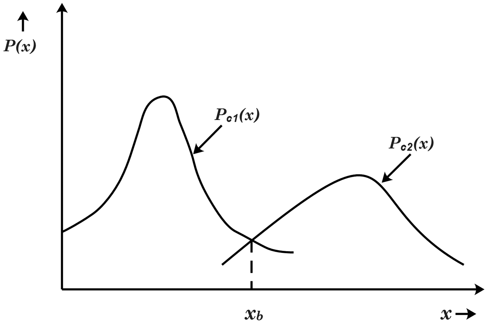

A sample with feature value x < x_b has P_c1(x_b) dx > P_c2(x_b) dx. It can be classified as belonging to class C1. On the other hand, a sample with feature value x > x_b has P_c1(x_b) dx < P_c2(x_b) dx. It can be classified as belonging to class C2. Thus, x = x_b constitutes the classification boundary.²⁷ The procedure has been directly extended to multiple classes and features of Bayes classifier by Hemantha et al.²⁸

In this study, the feature vector which comprises of selected features from decision tree is treated as an input to the Naïve Bayes classifier and the obtained results are discussed in “Feature selection and classification” section.

Results and discussion

Statistical features extraction

From the acceleration data, descriptive statistical features like skewness, mode, standard error, maximum, minimum, range, sum, mean, standard deviation, median, sample variance, and kurtosis are assessed to serve as features. These parameters are referred to as statistical features and these will be treated as input to the J48 algorithm.

Feature selection and classification

The J48 algorithm used the data set for making the decision tree as a result of feature selection. The given data set of 160 samples fed to the algorithm and decision tree is illustrated in Figure 6. The rectangular blocks indicate classes (condition of the tool).

Figure 6.

Decision tree.

All extracted descriptive statistical parameters were used as input to the decision tree, significant features to be selected out of the extracted ones. As seen from Figure 6, the tree structure of different classes has been formed in such a way that when standard error is greater than 0.022357 it is classified as healthy, whereas when standard error is greater than 0.018736 and less than/equal to 0.022357 it is classified as flank wear condition and so on. The tool conditions (healthy, chipping, breakage, and flank wear) are represented as leaves in the tree. Out of 12 features, six features selected by decision tree such as mean, kurtosis, range, median, mode, and standard error are the significant features. These selected features are treated as input to the classifier. In this study, 40 samples were considered for each condition of the tool (for four classes 160 samples). These data were divided into two; training data set and testing data set. Sixty-five percent of the samples were used as training set and the remaining 35% (14 samples per each class) of the samples were used for testing the model. The comparison of the performances of the different classifiers has been carried out to select an effective and efficient classifier. Classification accuracies of the different classifiers are shown in Table 1.

Table 1.

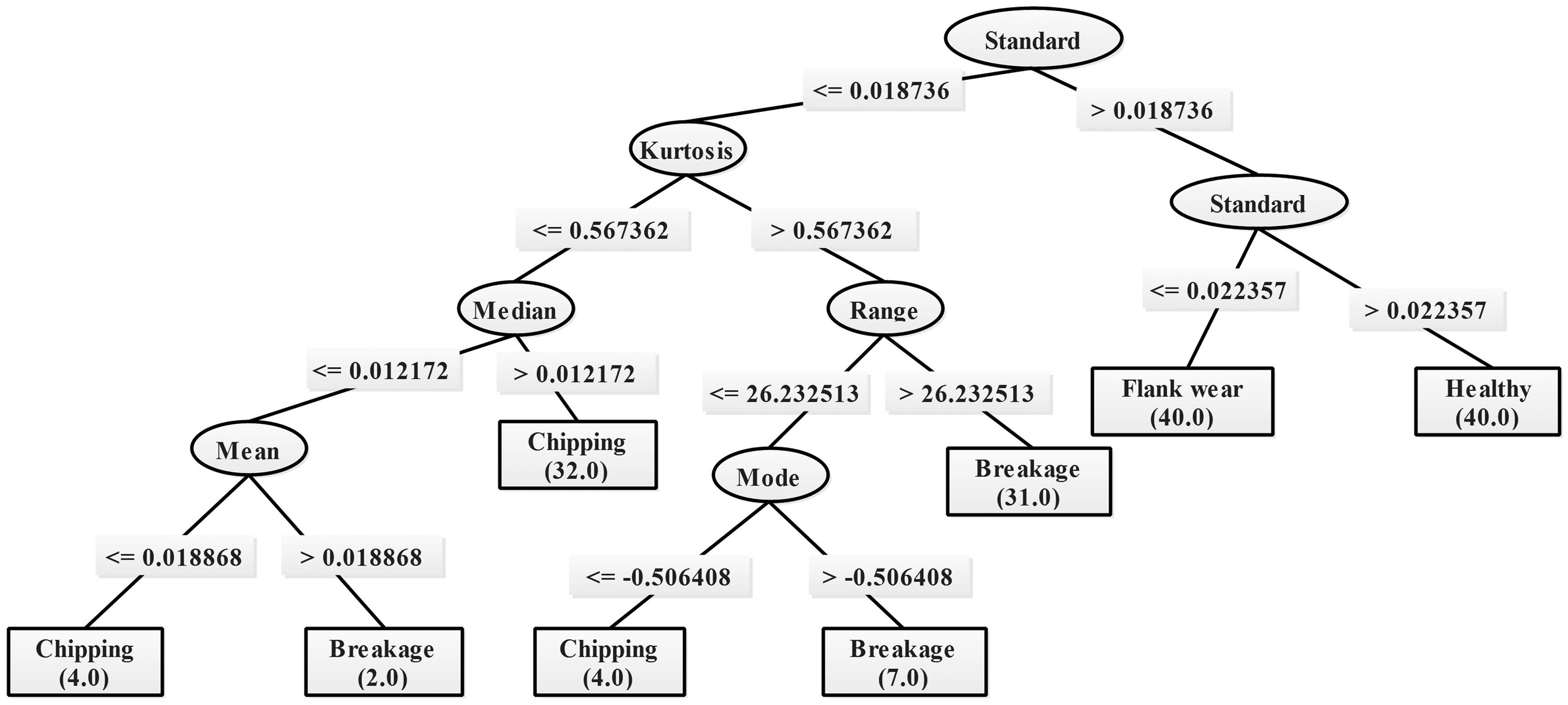
Performance of the different classifiers.

Classifier	Classification accuracy
Decision tree	Train set 94.23%
Decision tree	Test set 91.07%
ANN	Train set 95.19%
ANN	Test set 92.86%
Naïve Bayes	Train set 99.04%
Naïve Bayes	Test set 96.43%
SVM	Train set 98.08%
SVM	Test set 94.64%
K-star	Train set 96.15%
K-star	Test set 94.64%

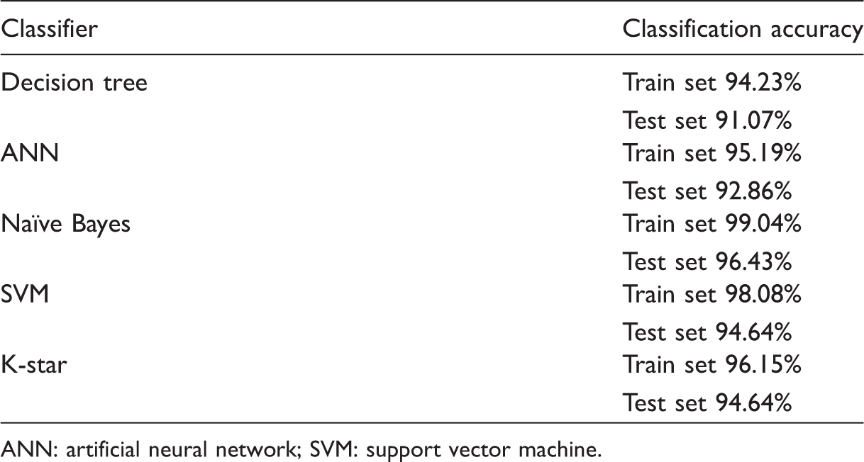
ANN: artificial neural network; SVM: support vector machine.

It is noted in Table 1 that the Naïve Bayes model has achieved a high classification accuracy (96.43%) as compared to other classifiers such as decision tree, artificial neural network, SVM, and K-star commonly used in the machine learning literature. Hence, the Naïve Bayes model is the best classifier in fault diagnosis of the face milling tool. Detailed classification of the tool conditions by the Naïve Bayes classifier is presented in Tables 3 and 4. Indira et al.²⁹ suggested a number of samples (less than 10 per each class) required to distinguish fault conditions in the area of machine learning approach. However, 40 samples per each class were used for classifying the face milling tool conditions in order to get a statistically stable classification accuracy. The parameters related to Naïve Bayes model are listed in Table 2.

Table 2.

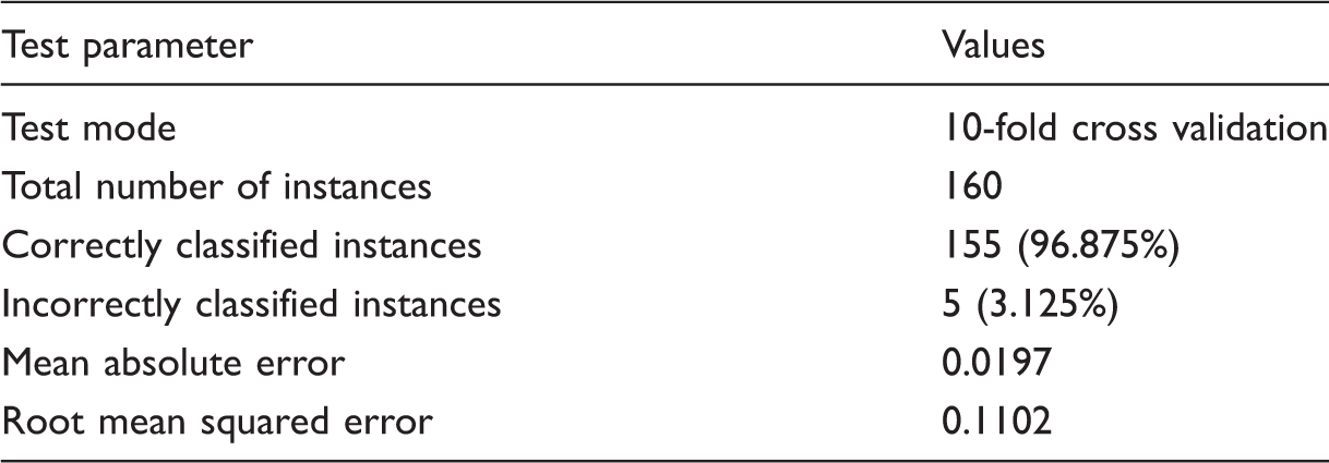
Naïve Bayes parameters for statistical features.

Test parameter	Values
Test mode	10-fold cross validation
Total number of instances	160
Correctly classified instances	155 (96.875%)
Incorrectly classified instances	5 (3.125%)
Mean absolute error	0.0197
Root mean squared error	0.1102

Table 3.

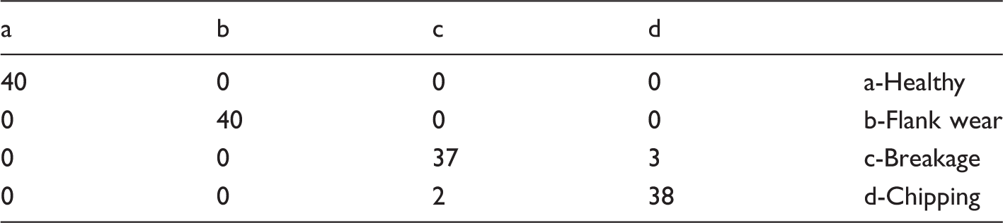
Naïve Bayes confusion matrix.

a	b	c	d
40	0	0	0	a-Healthy
0	40	0	0	b-Flank wear
0	0	37	3	c-Breakage
0	0	2	38	d-Chipping

Table 4.

Detailed accuracy classification with Naïve Bayes.

TP Rate	FP Rate	Precision	Recall	F-Measure	ROC Area	Class
1	0	1	1	1	1	Healthy
1	0	1	1	1	1	Flank wear
0.925	0.017	0.949	0.925	0.937	0.995	Breakage
0.95	0.025	0.927	0.95	0.938	0.995	Chipping

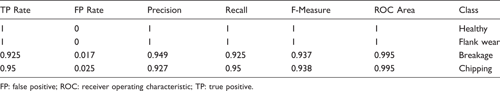
FP: false positive; ROC: receiver operating characteristic; TP: true positive.

Table 3 shows the confusion matrix of the Naïve Bayes classifier and diagonal elements represent the correctly classified instances. All instances which lie in the first row of the matrix belong to healthy condition, here all 40 instances (first row, first column element) were correctly classified as healthy. In a similar manner, all 40 instances of flank wear condition were also correctly classified. In case of breakage condition, 37 out of 40 instances were correctly classified as breakage, while three instances were misclassified as chipping and so on. Detailed classification accuracy of the Naïve Bayes model is as shown in Table 4, where the true positive rate (TP rate) and false positive rate (FP rate) indicate the significance in judging the quality of the model; for good classification TP rate implies “1,” while the FP rate implies “0.” For the given vibration signals, TP rate of healthy condition is 1 which indicates all 40 instances were correctly classified as healthy. In case of breakage condition, TP rate is about 0.925 which indicates 37 out of 40 instances were correctly classified as breakage, whereas three instances of breakage were misclassified as chipping which is represented by FP rate of 0.017 and so on. Here, out of 160 instances, five instances were misclassified by Naïve Bayes algorithm with the overall classification accuracy 96.9% for the given vibration signals. Ultimately, one can say that 100% (40 instances) of healthy instances were correctly classified, whereas none of the instances of fault conditions were represented as healthy. This can be accepted as a reasonably good performance of the classifier. Hence, the Naïve Bayes technique can be suggested for fault diagnosis of the face milling tool.

Conclusion

This paper dealt with the fault diagnosis of a multipoint cutting tool by using machine learning approach. Vibration signals pertaining to different conditions of the face milling tool were acquired and statistical features were extracted. Decision tree was used to select the significant features out of the extracted statistical features. The Naïve Bayes algorithm was used to classify the different conditions of the cutting tool. Based on the results and analysis, the following conclusions were drawn. Statistical features (standard error, mean, kurtosis, range, median, and mode) of vibration signals have served a good platform for classifying the tool conditions. The Naïve Bayes model has provided classification accuracy of about 96.9%, which is reasonably good and acceptable for the face milling process. This shows that machine learning technique is a promising approach for fault diagnosis of face milling tool and the combination of decision tree and Naïve Bayes techniques with statistical features can be recommended in applications of TCM system of the face milling process.

Footnotes

Acknowledgements

The authors acknowledge the Centre for System Design (CSD): A Centre of excellence at NITK-Surathkal for providing experimental facility and greatly acknowledge the support of Dr V. Sugumaran, Associate Professor, VIT University Chennai, for helping in machine learning theory for fault diagnosis application.

Declaration of conflicting interests

The author(s) declared no potential conflicts of interest with respect to the research, authorship, and/or publication of this article.

Funding

The author(s) received no financial support for the research, authorship, and/or publication of this article.

References

Teti

Jemielniak

O’Donnell

. Advanced monitoring of machining operations. CIRP Ann Manuf Technol 2010; 59: 717–739.

Dutta

Pal

Mukhopadhyay

. Application of digital image processing in tool condition monitoring: a review. CIRP J Manuf Sci Technol 2013; 6: 212–232.

Park

Ulsoy

. On-line flank wear estimation using an adaptive observer and computer vision, Part 2: experiment. J Manuf Sci Eng 1993; 115: 37–43.

LoCasto

LoValvo

Micari

. Tool wear measured by computer vision. C.S.M.E. Mech Eng Forum 1990; 3: 59–63.

Ryabov

Mori

Kasashima

. An in-process direct monitoring method for milling tool failures using a laser sensor. CIRP Ann Manuf Technol 1996; 45: 97–100.

Kuljanic

Sortino

. TWEM, a method based on cutting forces—monitoring tool wear in face milling. Int J Mach Tools Manuf 2005; 45: 29–34.

Tansel

Bao

Reen

. Genetic tool monitor (GTM) for micro-end-milling operations. Int J Mach Tools Manuf 2005; 45: 293–299.

Jemielniak

Arrazola

. Application of AE and cutting force signals in tool condition monitoring in micro-milling. CIRP J Manuf Sci Technol 2008; 1: 97–102.

Marinescu

Axinte

. A critical analysis of effectiveness of acoustic emission signals to detect tool and workpiece malfunctions in milling operations. Int J Mach Tools Manuf 2008; 48: 1148–1160.

10.

Rene de Jesus

Gilberto

Iván

. Driver current analysis for sensorless tool breakage monitoring of CNC milling machines. Int J Mach Tools Manuf 2003; 43: 1529–1534.

11.

Orhan

Camuşcu

. Tool wear evaluation by vibration analysis during end milling of AISI D3 cold work tool steel with 35 HRC hardness. NDT E Int 2007; 40: 121–126.

12.

Hsueh

Yang

. Tool breakage diagnosis in face milling by support vector machine. J Mater Process Technol 2009; 209: 145–152.

13.

Elangovan

Devasenapati

Sakthivel

. Evaluation of expert system for condition monitoring of a single point cutting tool using principle component analysis and decision tree algorithm. Expert Syst Appl 2011; 38: 4450–4459.

14.

Jantunen

. A summary of methods applied to tool condition monitoring in drilling. Int J Mach Tools Manuf 2002; 42: 997–1010.

15.

Dominik

Iwaniec

Lech

. Low frequency damage analysis of electric pylon model by fuzzy logic application. J Low Frequency Noise Vib Active Control 2013; 32: 239–252.

16.

Chiu

. Numerical assessment of rectangular side inlet/outlet plenums internally equipped with two crossed baffles using an FEM, neural network, and GA method. Low Frequency Noise Vib Active Control 2014; 33: 271–288.

17.

Tahmasebi

Rahman

Mailah

. Roll movement control of a spray boom structure using active force control with artificial neural network strategy. J Low Frequency Noise Vib Active Control 2013; 32: 189–202.

18.

Watany

Eltantawie

Abouel-seoud

. Application of an adaptive neuro fuzzy inference system for low speed planetary gearbox vibration control. J Low Frequency Noise Vib Active Control 2015; 34: 323–342.

19.

Sokolowski

. On some aspects of fuzzy logic application in machine monitoring and diagnostics. Eng Appl Artif Intell 2004; 17: 429–437.

20.

Sugumaran

Muralidharan

Ramachandran

. Feature selection using decision tree and classification through proximal support vector machine for fault diagnostics of roller bearing. Mech Syst Signal Process 2007; 21: 930–942.

21.

Painuli

Elangovan

Sugumaran

. Tool condition monitoring using K-star algorithm. Expert Syst Appl 2014; 41: 2638–2643.

22.

Wyse

Dubes

Jain

. A critical evaluation of intrinsic dimensionality algorithms. Pattern Recognit Pract 1980, pp. 415–425.

23.

Blum

Langley

. Selection of relevant features and examples in machine learning. Artif Intell 1997; 97: 245–271.

24.

Breiman

Freidman

Olshen

. Classification and regression trees, Boca Raton, FL: CRC Press, 1984.

25.

Gangadhar

Kumar

Narendranath

. Fault diagnosis of single point cutting tool through vibration signal using decision tree algorithm. ICAMME, NITK Procedia Mater Sci 2014; 5: 1434–1441.

26.

Soman

Diwakar

Ajay

. Data mining: theory and practice, New Delhi, India: PHI Learning Pvt. Ltd, 2006.

27.

Muralidharan V. Wavelet analysis of vibration signals for fault diagnosis. PhD Thesis, Karpagam University, Tamil Nadu, India, 2012.

28.

Hemantha

Kumar

Amarnath

. Fault diagnosis of bearings through vibration signal using Bayes classifiers. Int J Comput Aided Eng Technol 2014; 6: 14–28.

29.

Indira

Vasanthakumari

Sugumaran

. Minimum sample size determination of vibration signals in machine learning approach to fault diagnosis using power analysis. Expert Syst Appl 2010; 37: 8650–8658.

Fault diagnosis studies of face milling cutter using machine learning approach

Abstract

Keywords

Introduction

Experimental setup

Machine learning system

Feature extraction

Statistical features extraction

Feature selection

Decision tree (J48 algorithm)

Information gain and entropy reduction

Feature classification

Bayes classifier

Results and discussion

Statistical features extraction

Feature selection and classification

Conclusion

Footnotes

Acknowledgements

Declaration of conflicting interests

Funding

References