Sage Journals: Discover world-class research

Abstract

We examine the localized nature of COVID-19 pandemic spread in India. Through Gamma curve-fitting we observe that the infection patterns exhibit substantial variation across locations. Areas with larger male population and higher economic activity witness more cases. Economically-deprived districts experience higher mortality after controlling for the infections. Mobility in spatially contiguous locations is a significant determinant of new infections. Our study emphasizes the role of socioeconomic factors in explaining the variation across districts. The findings support the need for locally-specific policy, better medical infrastructure in socio-economically vulnerable localities and social-distancing measures in controlling the spread.

Executive Summary

The COVID-19 pandemic, a black swan event, created an unprecedented global health hazard and disrupted global economic activities. During the first wave of the COVID-19 pandemic, various governments announced lockdowns. India went under lockdown from 25 March 2020 for 21 days. These lockdowns disrupted the social fabric and economic activities. We examined the demographic and socio-economic determinants of COVID-19 infections and deaths across over 400 districts in India. Using statistical methods, we observed that the infection patterns demonstrate localized characteristics across districts. Areas with a larger male population and higher economic activity witnessed higher infection rates. Districts with more agricultural and backward caste populations and inferior latrine facilities experienced significantly higher mortality rates after controlling for infections and other variables, indicating that a higher concentration of economically deprived populations experience higher mortality. Mobility in spatially contiguous locations appears to be a significant determinant of new infections. Our study emphasizes the role of socio-economic factors in explaining the variation across districts. The findings support the need for locally-specific policy and social-distancing measures to control the spread.

Keywords

Socio-economic Localized Policy Measures Controlling Pandemic Spatial Autoregressive Regression COVID-19

Calls for a…national lockdown [in India] have…come from business leaders, international health experts and other senior politicians.

—BBC, 2021

[T]here are several problems in a lockdown situation [in India] that are more economic than medical.

—France24, 4 September 2020

India offers an interesting laboratory to test the variation in the COVID-19 pandemic spread: The nation offers a vast population promising a wide variety of climatic and socio-economic characteristics across its localities. The heterogeneous population and diverse social structure within the national boundaries present India as a useful case study to evaluate the impact of various socio-economic factors on the spread of the pandemic. According to BBC News, 10 worst affected districts in India were urban, accounting for 80% of deaths. High population density in urban areas, resulting in constraints on social distancing, (Alluri & Nazmi, 2020) is a plausible explanation.

The first COVID-19 case in India was reported on January 30, 2020. In the middle of September 2020, the daily reported cases peaked at about 98,000. The policy responses were multifold. Initially, virus screening started at airports through inbound international travellers (Kamath et al., 2020; Laxminarayan et al., 2020). While health experts like Dr Anthony Fauci, a public health expert from the US, called for a ‘nationwide lockdown’ (BBC, 2021), economic experts in India considered localization of lockdowns as a better policy (Choudhury, 2021). Testing and contact-tracing travellers, imposition of lockdown and government advisory on social distancing were effective in checking the spread of this deadly virus in India. However, the blanket policy measure applied almost uniformly on the national scale had socio-economic repercussions. The underprivileged segments of society were the worst hit (World Bank Group, 2020). The plight of the migrant labourer community that went through a forced exodus from urban hubs to villages led the prime minister to ‘ask for forgiveness’ for the sweeping lockdown policy (BBC, 2021).

In the situation of a predicament, and conflicting policy recommendations, a confused and frenzied policy response is natural. After the COVID waves subsided, economists estimated the costs of national-level lockdowns (Engage, 2021). The costly economic repercussions alone, however, are inadequate evidence to critique the national lockdown policy, as the lockdown was considered a necessity by health experts. A pertinent research question relates to the debate of whether a localized lockdown could have partially averted the adverse economic outcomes of a national lockdown.

In this study, we highlight the localized nature of the pandemic and argue that localized responses can be more effective in balancing the ill effects of national-level restrictions. Our approach is to explain the spread of the pandemic using localized socioeconomic, mobility and climatic characteristics. We apply ordinary least-squares (OLS) and spatial regression models to geo-enriched, district-level data on infections and deaths. Our findings support the role of socio-economic factors in the spread of the pandemic and point towards the efficacy of social-distancing measures and hygiene infrastructure in reducing the spread.

Our study adds to an emerging body of knowledge related to the spread of COVID-19 infections and deaths. We consolidate earlier findings into a robust empirical framework and introduce additional variables. Using geo-enriched data on demographics (e.g., age, gender, caste) and socio-economic behaviour across different climatic zones of a diverse nation.

The rest of the article is organized as follows. The next section provides a synthesis of the emerging literature on COVID-19. We then delve into the data description and explain our choice of empirical methods: (a) OLS regression and (b) spatial autoregressive regression (SAR). Subsequently, we present and discuss the result of our analysis. The last section provides the concluding remarks.

BACKGROUND

Since the outbreak of the COVID-19 pandemic in early 2020, many researchers have investigated factors associated with the spread of this virus. The findings are mixed, and the reasons for virus transmission are not completely understood (Ghosh et al., 2020). Some factors examined—that are associated with the spread of the virus in urban centres—include social distancing (Tammes, 2020), population density (Ahmadi et al., 2020; Coşkun et al., 2021; Hamidi et al., 2020; Kodera et al., 2020; Liu, 2020; Mishra et al., 2020a), climatic factors (Ahmadi et al., 2020; Coşkun et al., 2021; Ghosh et al., 2020; Gupta et al., 2020; Kodera et al., 2020; Pramanik et al., 2022; Rashed et al., 2020), demographic factors (Sannigrahi et al., 2020), ethnicity (Khunti et al., 2020), age-demographic (Liu et al., 2020), racial, caste and ethnic factors (Holtgrave et al., 2020; Nandi et al., 2020), slum and non-slums areas (Malani et al., 2020), and the role of built and social environmental (Hu et al., 2020).

Tammes (2020) reported that the spread of COVID-19 in highly dense urban pockets in the UK dropped from the highest to the lowest after applying social distancing measures for four weeks. In the US, Hamidi et al. (2020) reported that larger metropolitan areas have higher infection and mortality rates. However, counties with high density were found to have fewer infections, possibly due to better health facilities. The study proposes connectivity to be more important to the spread of the virus than population density. Mishra et al. (2020a) assigned the highest weight to the population in the Covid Vulnerability Index developed for the top four metropolitan cities of India—Delhi, Mumbai, Kolkata and Chennai. However, Liu (2020) found density to be negatively related to the spread of the COVID-19 pandemic in the early stages in China. Sun et al. (2020) found that the spread of COVID-19 under the strict Chinese lockdown measures had a significant negative correlation with longitude and latitude; however, the study failed to establish any correlation with population density.

Some studies evaluated the impact of climatic conditions on the spread of the virus. In the cold climatic conditions of Russia, Pramanik et al. (2022) found temperature seasonality and climatic zones to have an impact on the transmission and spread of COVID-19. Kodera et al. (2020) showed that higher temperatures and absolute humidity are associated with a decrease in infections and mortality rates in Japan. Gupta et al. (2020) reported that hot and dry regions in the lower altitudes of India are more likely to be impacted by COVID-19. However, Ghosh et al. (2020) concluded that climatic factors (temperature, humidity and wind speed) alone are not sufficient to explain the spread of COVID-19 in London.

Others evaluated the impact of both climatic factors and population density. Ahmadi et al. (2020) find population density, interprovincial movement and climatic factors (humidity, wind movement and solar radiation) to have an impact on the spread and survival of the virus. Coşkun et al. (2021) reported that population density and wind impacted the spread of the COVID-19 virus in Turkey but failed to find an effect of temperature, humidity, etc. Rashed et al. (2020) reported the maximum absolute humidity, ambient temperature and population density to be important factors in the spread and decay patterns of the COVID-19 pandemic in Japan.

Additional factors associated with the spread of COVID-19 have also been evaluated. Liu et al. (2020) reported that the mortality of elderly patients is higher than that of young and middle-aged patients from COVID-19 infections. Higher mortality from this virus has been reported in the male population (Jordan et al., 2020; Laxminarayan et al., 2020). Holtgrave et al. (2020) and Khunti et al. (2020) reported linkages between racial and ethnic factors with the COVID-19 spread and mortality in developed countries. They suggest that these findings are also relevant to Africa and South Asia and report that ethnic minorities faced several disadvantages due to low-paid jobs and poor housing. For Brazil, Tavares and Betti (2021) developed two pandemic indexes to show considerable ethnic and regional inequality. In India, Tamrakar et al. (2020) reported that deprived sections of the society, like Scheduled Castes (SCs), are more vulnerable to infection. Nandi et al. (2020) found that districts in eastern and central India (Uttar Pradesh, Bihar and Madhya Pradesh) with a high rural, SC and Scheduled Tribe (ST) populations have a high risk of COVID-19 infections due to poverty and limited access to health care. Patel et al. (2020) reported that SC and ST populations are the most deprived caste in India, living in slums in urban areas and having poor access to water and sanitation. Tamrakar et al. (2020) further highlighted that these deprived sections of the society in India are more vulnerable to infection. Malani et al. (2020) showed that in Mumbai, India, there are sustainably high infection rates in slums compared with non-slum areas. This may be due to the high density and high vulnerability of these deprived sections of the society due to caste factors and limited options of social distancing. Auerbach and Thachil (2021) studied the impact of COVID-19 on the urban slum dwellers in North India and found that some slums have better managed the government guidelines like social distancing than others. Wan and Su (2016) showed in China, poor housing conditions are more responsible than socio-economic disadvantage in poor health conditions.

The COVID-19 spread may have originated in cities, but it is believed that due to migrant workers returning to the rural areas, it spread quickly in rural areas as well in India. Maintaining social distancing in agrarian rural India is difficult for various reasons, including common sources of water and latrine (Mishra et al., 2020b). An article in The New York Times points out the defiance of COVID-19 rules (e.g., social distancing, wearing masks, getting tested and not reporting illness) in rural India. This is also attributed to the fact that agricultural labour depends on daily wages and could not afford quarantine for the entire family in case of any member testing positive (Singh & Gettleman, 2020). Even in a developed country like the US, agricultural workers are considered susceptible to COVID-19 infection due to poor sanitation and working conditions that do not support social distancing and other infection protection measures (Handal et al., 2020).

There has been a burgeoning body of literature that explores various factors that impacted the spread and mortality across the globe due to COVID-19. This literature is evolving, but scientific endeavours to study its spread are limited and few, especially in populous India. Our article consolidates all the earlier findings into a robust empirical framework. We also introduce some new variables related to socio-economic behaviours (e.g., access to banking, mobile phone and latrine facilities).

RESEARCH METHODOLOGY

Data

The data summary and sources are shown in Table 1. We collected data for this study from multiple sources. The COVID-19 data for the 412 districts of India were collected from www.covid19india.org/. These data were available on a daily frequency since the reporting of the first case in India (on 30 January) and we analysed daily reported infections until 13 October 2020. The number of cases varied within a broad range of 141 (East Sikkim) to 3.9 mi (Ahmedabad area).

Table 1:

Data Summary and Description.

Variable	Description	Source	Mean	Min	Max	Std. Dev.
Cases_Total	Total number of COVID-19 Cases	covidindia.org	30,0924	141	3,904,053	445,851
Cases_DaystoFirst*	Number of days until the first case was recorded	covidindia.org	84	1	194	34
Moisture**
3Arid	< −66.7	ICAR-CRIDA	0.08	0	1	0.27
Dry sub-humid	−66.6 to −33.3	ICAR-CRIDA	0.25	0	1	0.43
Humid	−33.3 to 0	ICAR-CRIDA	0.11	0	1	0.31
Moist subhumid	0 to 20	ICAR-CRIDA	0.06	0	1	0.23
Per-humid	20.1 to 99.9	ICAR-CRIDA	0.13	0	1	0.33
Semi-arid	> 100	ICAR-CRIDA	0.38	0	1	0.49
Irrigatearea	Net irrigated area (%)	ICAR-CRIDA	46	0	100	31
GIS Data: Based on a polygon drawn within 30-minute driving distance around each district centre
POPDEN	Population density per square km (2018)	ESRI	1,899	41	26,032	2,173
POP	Population (2018)	ESRI	47,6690	83	6,476,347	609,115
PC30TO45	% Population aged between 31 and 45 years (2012)	ESRI	0.20	0.15	0.50	0.02
PC45TO60	% Population aged between46 and 60 years (2012)	ESRI	0.12	0.08	0.50	0.03
PC60PLUS	% Population aged beyond 60 years (2012)	ESRI	0.09	0.04	0.50	0.03
MALEWORKERPC	% of male workers in the population (2012)	ESRI	0.70	0.47	0.89	0.09
PC.ST	% of Scheduled Tribe in the population (2012)	ESRI	0.14	0.00	0.99	0.27
PC.SC	% of Scheduled Caste in the population (2012)	ESRI	0.15	0.00	0.61	0.09
PPPC	Average purchasing power per capita (₹) (2020)	ESRI	91,275	23,230	280,560	40,933
BANK	Number of persons availing banking services (2012)	ESRI	52,588	0	832,461	75,719
MOBILE	Number of persons owning a mobile phone (2012)	ESRI	49,223	0	733,744	73,009
GOODLATRINE	Number of people with access to good latrine facility (2012)	ESRI	53,611	0	1,085,880	98,394

Note: This table describes the data on COVID-19 infections across 412 districts of India between 4 March and 13 October 2020. ^**The moisture data are based on earlier works of Thornthwaite and Mather (1955) and Krishnan (1988).

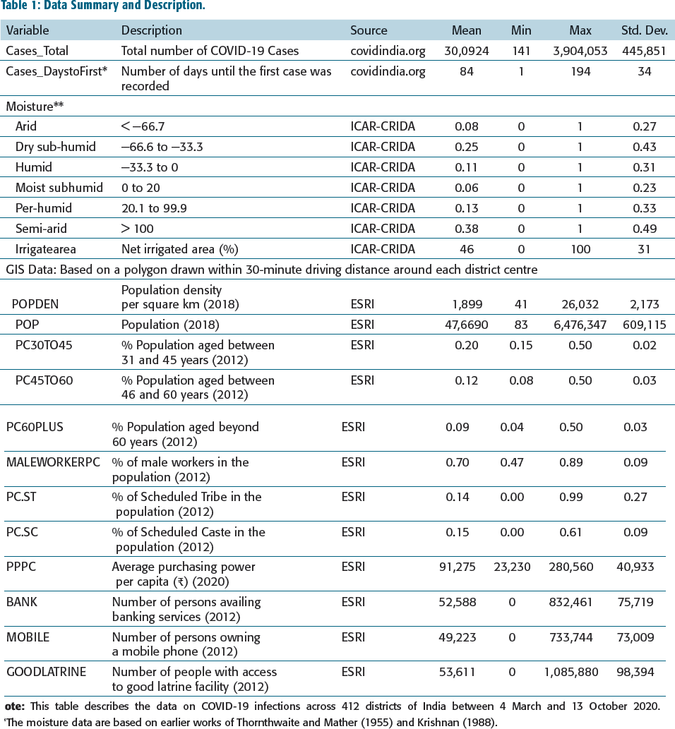
Different locations were at different stages of the pandemic cycle, and we also counted how many days it took a location to record its first case since the start date of data. The longer the Cases_DaystoFirst, the earlier a location is in the stage of the pandemic. In our sample, this duration varied between 1 day (e.g., Thrissur, Kerala) and 194 days (Wokha, Nagaland), indicating regional heterogeneity in the spread of this virus across the country. These locations are considered to be 46% net irrigated. We construe the measure of net irrigation as a reflection of agricultural activity.

Humidity-based¹ climatic zones in India are classified as arid, semi-arid, dry sub-humid, moist sub-humid, humid and per-humid (ICAR-CRIDA, 2014; Thornthwaite & Mather, 1955; Venkateswarlu et al., 2014). Later, these zones were simplified by Krishnan (1988). These two studies map a sample of representative cities to specific climatic zones. We also draw an alternative climatic classification from Bhatnagar et al. (2019), which includes temperature and sunlight data beyond humidity in the zone classification. We cannot identify a one-to-one representation of the districts used in the sample in the climatic zone studies. Therefore, we identified the centroids of the cities (included in the climatic zone studies) and districts analysed in our studies. Using geographic information system (GIS), we found the nearest locations (identified with one of the eight climatic zones in Bhatnagar et al. (2019)) and assumed that the subject city broadly falls within the same zone. Most locations in our sample belong to the semi-arid (38%) climate type, followed by dry sub-humid (25%).

We are also interested in the demographic and socio-economic behaviour of the population in these localities. Unfortunately, most of these data are not available at the desired level of granularity. Some of the desired data are available only in geocoded form from the Environmental Systems Research Institute (ESRI).² First, we find the centroid coordinates of a district using GIS technology. For representative characteristics of a district, we draw boundaries surrounding the district centres. Unlike the political boundaries of a district, a polygon surrounding a city centre is more representative of the urban characteristics, as district boundaries also include rural areas. The most intuitive polygons would be geometric shapes. However, district maps are irregularly shaped, and populations may have spread in specific directions. Unlike a geometric polygon, transportation routes may vary drastically across localities. The driving-time-based geographic boundary incorporates information on road availability, directionality and average vehicle speed, etc. As a result, polygon boundaries characterized by driving time are a more realistic representation of the local population rather than geometrically drawn polygons.

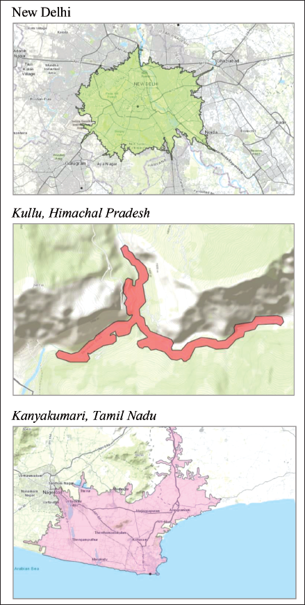
We draw a 30-minute driving time polygon around each city centre to identify the polygons around cities. Such a method has been used in the past by Das et al. (2018) and Das et al. (2020). For illustration purposes, we provide driving-time-based polygons around three representative district-centres in Figure 1. New Delhi is broadly a radial polygon, given the flat landscape and few geographic barriers that prevent the city from expanding. The driving distances around the city are broadly the same in all directions. Kullu (Himachal Pradesh) presents a star-shaped polygon due to the shape of the valley surrounded by mountains. Kanyakumari, a cape city, only expands northwards from the city centre. Clearly, the geometric polygon will be misrepresentative in the last two cases discussed above and will provide data biased towards rural or uninhabited areas.

Figure 1:

Source: ESRI and authors.

ESRI aggregates social behaviour and demographic data from multiple sources and geocodes them. This enables us to collect local data related to the polygons drawn around district centres as described above.

The population in the polygons varies between 41 (Siang, Arunachal Pradesh) and 6.5 mi (Ahmedabad area). Nearly 60% of the population (based on 2012 data) is below the age of 15, followed by 30–45 years (20%), 45–60 years (12%) and 60+ (9%). However, the age groups vary substantially across the districts. The percentage of males in the working population averages at 70%, ranging from 47% (mostly in Himalayan districts) to and 90% (mostly in plains). The percentage of STs varies drastically between 0% (some districts in Punjab and Haryana) and 99% (districts in Gujarat, Madhya Pradesh and Rajasthan). The distribution of the SC population is similarly dispersed between 0% and 61% across the districts. However, the geographic distribution of the SC population exhibits marked differences from ST, with some of the highest SC populations in Uttar Pradesh, Punjab, Maharashtra, etc., and the lowest in Himalayan districts.

Access to good latrine facilities varies from very low (e.g., Himalayan districts, Kutch Gujarat, etc.) to high (in major metro areas). Similarly, the purchasing power per capita (2012) varies from the lowest of around ₹23,000 ($400) in some districts of Bihar, Uttar Pradesh and Mizoram to around ₹281,000 ($5,000) in some districts of Maharashtra, Gujarat, Andhra Pradesh and Sikkim. Access to mobile phones and bank accounts (2012), too, varies drastically between zero and around 800,000 individuals across districts.

A limitation of our data is that the latest GIS-based social data available to us are eight years old. These variables may have witnessed changes since then. As long as the comparative status across the districts has not changed drastically since then, their inclusion in the empirical analysis is still helpful.

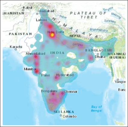
The synthesis of the data description provides a heterogeneous distribution of different social variables across the locations. There is some correlation between climatic zones and demographic variables. For example, we should expect a more working-age population in metro areas mostly located in semi-arid or semi-humid plains. However, some other variables exhibit distinct patterns. For example, locations dominated by the ST population exhibit a low SC population. Also, mountainous regions seem to have the lowest access to latrine facilities, as expected. The variation in access to banking facilities and mobile phones is almost identical. Figure 2 shows the heat map of the population with access to mobile phones. Although more intense around big metros, the areas of concentration are spread across the nation.

Figure 2:

Heat Map of Mobile Users (2012).

Method

We conduct our analysis in three steps. First, we analyse the infection curves across locations. Then, using (a) OLS regression (OLS) and (b) spatial regression models, we analyse the determinants of COVID-19 infections across the nation.

The Infection Curve at the State Levels

First, we develop an infection case curve for each district. However, due to data artefacts, it was more feasible to develop these curves at the state level. We apply curve-fitting techniques to the new COVID-19 cases for each State and Union Territory (UT) in India. According to the Kermack and Mckendrick (K-M) model, such pandemic cases follow a gamma curve (Kermack & Mckendrick, 1927). The theoretical basis of the model has been widely studied and further developed (Raissi et al., 2019; Tong et al., 2016). The model has been used in many areas, such as studying the spread of influenza (Khalil et al., 2012), plant diseases (Segarra et al., 2001), HIV/AIDS (Chin & Lwanga, 1991; Mertens & Low-Beer, 1996) and computer worms (Yao et al., 2018).

According to the K-M model, subjects of a pandemic belong to one of the three states³: Susceptible (S), Infectious (I) and Removed (R). Assuming the population to be fixed in the short run, the total population at time t is N = S + I + R. A susceptible person has a specific probability of being infected after coming in contact with an infected person. An infected person recovers at another specific rate per unit of time. Studies have shown that a system of equations⁴ could be developed and solved to show that infection cases follow a Gamma curve over time. Such curves have become prevalent in public discourses in recent months. Gamma curves for new infections have a long right tail and can be described as a function of time t as $\frac{1}{θ^{k}, Γ (k)} t^{k - 1} \cdot e^{- t}$ , where k defines the shape and defines the scale of the curve. Figure 3 shows how the gamma distribution curve varies with the shape parameter. As such $\frac{1}{θ}$ is termed the rate parameter. In particular, the shape parameter k defines the steepness of the pandemic curve.

Figure 3:

Gamma Curves in an Increasing Order of the Shape Parameter (1: 10, left: right).

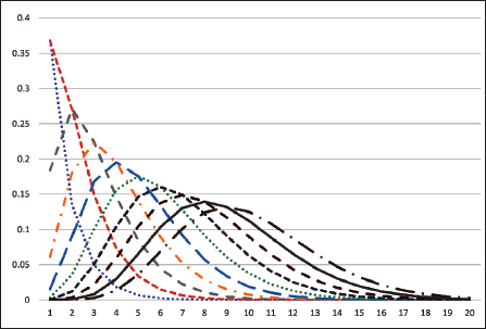
For example, owing to different shape parameters, in one location, the pandemic may rise and fall steeply, while it may rise fast but take much longer to fall. The rate parameter is related to the duration of the pandemic. For example, two locations may follow the same shape, but the timeline over which the shape is realized may be shorter in one location and longer in another. Note that in our study, we assume that the curve is still in the first wave of the pandemic. Therefore, locations said to have experienced the second wave until our date of data collection (mid-October 2020) may not fit well with the theoretical model.

We use a nonlinear least-squares regression model to estimate the parameters of a suitable gamma curve and use optimization techniques to maximize the fit with the observed data. The technique normalizes the data into standard probability distributions. In particular, we minimize the root-mean-squared error of the cumulative distribution function (CDF). On the best-fit curve, we estimate the phase of the pandemic, which depends on the location of the latest data on the curve. For example, a 99% cumulative probability density denotes the near-end of the first wave of the pandemic. We examine the correlation between state-level infection curve parameters and demographic indicators.

OLS Regression Models at District Level

First, we conduct OLS regression models for cumulative infections and deaths related to COVID-19 at district levels. Our model takes the following form:

\ln (Infections) = α + β_{1} Phase + β_{2} Climate + β_{3} X + ε

(1)

\ln (Deaths) = α + β_{4} Infections + β_{5} Climate + β_{3} X + ε

(2)

In these equations, Climate refers to a matrix of climatic-zone dummy variables, and X denotes a matrix of GIS-based local demographic indicators and other controls. The corresponding betas depict vectors of the corresponding regression coefficients. As infections started on different dates across locations, the locations may be at different Phases of the infection curve. We control for the Phase by including how delayed the first infection was observed at a location (Cases_DaystoFirst). In the model for deaths, we replace the phase with Infections to analyse the death based on infections.

Spatial Regression Models at the District Level

OLS models consider geographic independence in the dependent variables. However, the local mobility of people is a known determinant of the infection-spread. The spatial econometric technique allows us to capture the effect of mobility. Our motivation for applying spatial econometrics is two-fold. First, such models are known to improve the explanatory power, and second, they help us highlight the importance of localized policy measures.

Our spatial models help identify the spread of the dependent variable (ρ = ‘spatial auto-regression’ coefficient—explained in detail in the following paragraphs) from one point to the points in its neighbourhood. If we hypothesize that—at least partially—local mobility of the population adds to the spread of the pandemic, we should expect a positive and significant spatial autoregression in the infections models, but should observe a weaker effect in the model for deaths.

In the next step of the analysis, we apply SAR models. Spatial regression models extract information from the dependent variable in neighbouring locations and use their combination as an independent variable. The combination is carried out using a spatial weight matrix W applied to different spatial lags (i.e., different levels of the neighbourhood, diminishing with distance) of the dependent variable (spatial autoregression). The inclusion of W in the models implies that beyond the local characteristics, infections are also endogenously influenced by neighbouring locations, although their influence diminishes with distance. Given the n number of districts in our sample, we develop an n × n matrix of Euclidean distances between assets using their geographic coordinates (i.e., latitude and longitude), where n is the number of districts included in our study. Thus, each district has (n−1) neighbours. Then, distances in the weight matrix are calculated by the geographic coordinates and inversed to account for the diminishing influence of distance. In each row, we divide individual distances by the sum of all the distances in the row. This renders the weight matrix more sensitive to the nearer neighbours. The resulting SAR model can be interpreted as follows:

y = ρ W y + α t_{n} + Z β + ε

(3)

Here, $l_{n}$ is a constant-term vector of ones and Z is a set of exogenous explanatory variables. The implied data-generating process for the above equation is as follows:

\begin{matrix} y = {(I_{n} - ρ W)}^{- 1} (α l_{n} + Z β) + {(I_{n} - ρ W)}^{- 1} ε \\ ε \sim N (0, σ^{2} I_{n}) \end{matrix}

(4)

where I_n is an n-dimensional identity matrix, y denotes the dependent variable (infections or deaths) and Z denotes the set of independent variables from Equations (1) and (2). The spatial coefficient ρ measures the spatial autoregressive effect of the dependent variable. A statistically significant (and positive) ρ signifies that the dependent variables (infections, or deaths) are spatially correlated and reinforce each other (Das et al., 2020). High incidence rates in a location will put positive pressure on neighbouring locations. ρ captures those micro-location-specific variables that were omitted from the base OLS model but are associated with the incidence of COVID-19-related deaths or infections. When modelling infections beyond the omitted micro-location attributes, the mobility across neighbouring locations (that the baseline OLS models are unable to capture) is a plausible explanation for the significant spatial autoregression coefficient (ρ). However, mobility offers a weak explanation for deaths.⁵ Therefore, we should expect the ρ to be larger and more significant in the infection models.

RESULTS AND DISCUSSION

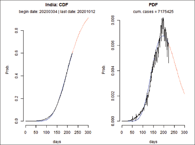
Figure 4 shows our attempt to fit a gamma curve for the entire India based on the CDF and probability distribution function (PDF).

Figure 4:

Fitting a Gamma Curve to the National Infections Data.

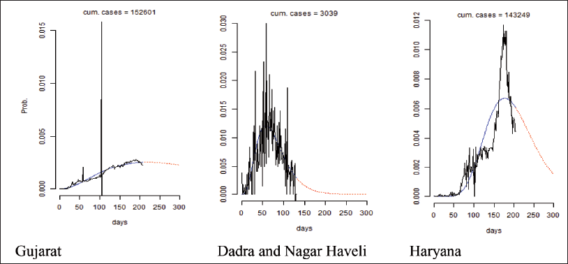
We also estimate the best-fit gamma curves separately for different states and UTs. As depicted in Figure 5, the gamma curves vary across the states. The curve has a fatter right tail in Gujarat, a steep right tail in Dadra and Nagar Haveli, and a relatively symmetric curve in Haryana. This points towards the heterogeneity of pandemic progression across different states. As discussed in the data section, different parts of the nation are characterized by different demographics, climatic and socio-economic characteristics. The differing nature of the Gamma curve across states and UTs suggests the need for localized policy measures rather than a uniform, national-level resolution.

Figure 5:

Variation in the Gamma Curve Across States.

Furthermore, we examine the correlation between the gamma curve parameters and some state-level characteristics, as presented in Table 2.

Table 2:

Correlation of Infection Curve Parameters and State Level Attributes.

	2011 Population (mi)	2011 Density per sq km	2012 PercentBPL	2015 Health Centres
Panel A: Summary
Average	34,596	1,098	18	5,106
Min	64	17	1	18
Max	199,812	11,320	40	24,791
Stdev	44,452	2,389	12	5,943
Panel B: Correlations	2011 Population	2011 Density per sq km	2012 PercentBPL	2015 Health Centres
2011 Population
2011 Density per sq km	−0.12
2012 PercentBPL	−0.01	0.12
2015 Health Centres	0.95	−0.21	−0.04
Shape (gamma curve)	0.14	0.10	0.22	0.10
Rate (gamma curve)	0.01	0.07	0.15	−0.05

Note: The state-wise data are extracted from NITI Aayog. Gamma curve parameters are based on authors’ curves fitted on state-level data extracted from www.covidindia.org. PercentBPL denotes the per cent of population below the poverty line.

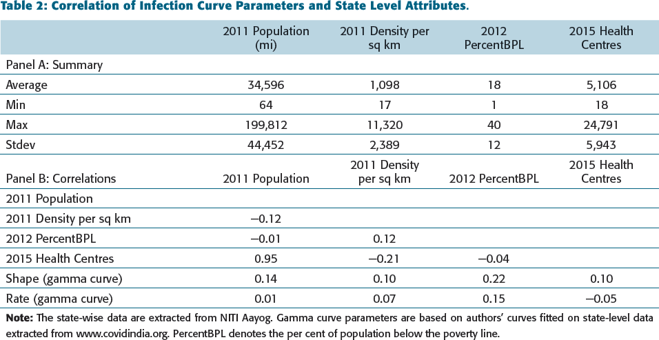
Panel A of Table 2 provides the state-level descriptive statistics. Panel B shows the correlation matrix. We are primarily interested in the correlation of gamma curve parameters (shape and rate) with other variables. Table 2 provides preliminary evidence that infection cases are correlated with demographic variables such as population, poverty (below the poverty line population) and availability of health facilities.⁶ The correlation analysis of state-level characteristics and gamma curve parameters (shape and rate) hints at the role of population, poverty and medical facilities in the pandemic spread. Similar to our findings, Nandi et al. (2020) found that poverty and medical infrastructure at the district level in India impact the risk of the COVID-19 pandemic. However, unlike previous research (e.g., Ahmadi et al., 2020; Coşkun et al., 2021; Hamidi et al., 2020; Kodera et al., 2020; Liu, 2020; Mishra et al., 2020a), we were not able to establish a correlation between COVID-19 and population density. This finding is in line with that of Sun et al. (2020).

While the bi-variate state-level correlations support the view that the infection curve is associated with demographics, it offers a small sample of 35 observations. Therefore, in the next step, we analyse the data of 412 districts for which sufficient data are available, both on infections and demographics. Due to data availability issues, we cannot match the state-level variables exactly at the local polygon levels. Besides, we were not successful in fitting gamma curves to several districts. However, we extract similar geocoded demographic data using GIS. Therefore, at this stage, we focus on modelling the number of total infections and deaths at the district level. An advantage of district-level geocoded data is that it affords us a wider set of potential determinants of infections, including age, income, occupation, social stratum, climate, consumption pattern, among others.

The results of the OLS model are shown in Table 3. Many previous studies have shown the impact of climatic factors on the spread and mortality due to COVID-19 (e.g., Kodera et al., 2020; Kroumpouzos et al., 2020; Pramanik et al., 2022). Therefore, we examine two sets of climatic controls in our models of infection and death cases. The first set includes humidity-based climatic controls. The second is based on the climatic zone proposed by Bhatnagar et al. (2019). Although most climatic zones are statistically insignificant in explaining the infections or deaths (similar to Ghosh et al. (2020)), some other variables are consistently significant across the two climatic sets of controls.

Table 3:

OLS Models.

	Ln(Cases)	Ln(Deaths)	Ln(Cases)	Ln(Deaths)
(Intercept)	5.14 (2.50) ^*	−2.72 (2.95)	2.81 (2.62)	−1.85 (2.98)
Ln(Cases)		0.62 (0.07) ^***		0.58 (0.07) ^***
Ln(Cases_DaystoFirst)	−0.43 (0.16)^**		−0.25 (0.15)
Ln(POP)	0.35 (0.14) ^*		0.50 (0.15) ^***
PC30TO45	−17.09 (6.26)^**	−5.77 (8.62)	−8.60 (6.35)	3.35 (8.72)
PC45TO60	20.44 (7.20) ^**	−11.03 (9.98)	3.67 (7.53)	−9.51 (10.36)
PC60PLUS	−1.80 (4.85)	1.68 (6.77)	5.27 (4.94)	−4.17 (6.86)
MALEWORKERPC	1.87 (0.89) ^*	2.25 (1.21) ^.	1.41 (0.84) ^.	1.72 (1.14)
PC.ST	−0.95 (0.38)^*	−0.88 (0.53)^.	−0.58 (0.40)	−0.25 (0.54)
PC.SC	−1.57 (0.86)^.	3.12 (1.19) ^**	−0.75 (0.88)	4.34 (1.22) ^***
Ln(PPPC)	0.46 (0.20) ^*	0.29 (0.27)	0.51 (0.22 ) ^*	0.12 (0.29)
Ln(BANK)	0.71 (0.22) ^**	1.07 (0.31) ^***	0.59 (0.23) ^*	0.13 (0.33)
Ln(MOBILE)	−0.58 (0.27)^*	−0.67 (0.36)^.	−0.60 (0.27)^*	0.12 (0.36)
Ln(GOODLATRINE)	−0.25 (0.16)	−0.55 (0.22)^*	−0.24 (0.17)	−0.40 (0.23)^.
IrrigateareaPC	<0.001 (<0.001)	0.01 (<0.01) ^*	0.01 (0.00) ^*	0.01 (<0.01)^*
Climate (Humidity) Classification
Dry sub-humid	0.02 (0.25)	−0.56 (0.35)
Humid	−0.50 (0.30)	−1.26 (0.43)^**
Moist subhumid	0.30 (0.33)	−0.37 (0.46)
Per-humid	−0.95 (0.32)^**	−2.09 (0.46)^***
Semi-arid	0.22 (0.23)	−0.35 (0.32)
Climate Zones
Zone 1 (e.g., Dehradun)			0.03 (0.23)	−0.30 (0.32)
Zone 2 (e.g., Jaipur)			0.34 (0.20)^.	0.34 (0.28)
Zone 3 (e.g., Mumbai)			0.74 (0.19) ^***	−0.62 (0.27)^*
Zone 4 (e.g., New Delhi)			1.68 (0.80) ^*	−1.68 (1.13)
Zone 5 (e.g., Imphal)			−0.66 (0.42)	−2.76 (0.58)^***
Zone 6 (e.g., Srinagar)			0.53 (0.45)	1.19 (0.62) ^.
Zone 7 (e.g., Dibrugarh)			−1.40 (0.29)^***	−2.83 (0.41)^***
Zone 8 (e.g., Shillong)			−0.07 (0.46)	−0.62 (0.61)
R ²	0.51	0.60	0.55	0.64
Adj. R²	0.48	0.59	0.52	0.62
Num. obs.	412	412	412	412

Notes: This table presents OLS regression models for notes:^***p < .001; ^**p < .01; ^*p < .05; p < .1.

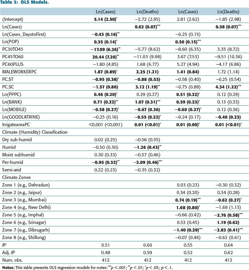
The OLS models support the earlier finding related to more cases in highly populated localities. Such localities may restrict social distancing measures, and their health infrastructure may be stressed when infection rates are as high as in COVID-19. In line with past research (e.g., Jordan et al., 2020; Laxminarayan et al., 2020; Livingston & Bucher, 2020), we found that districts having a high percentage of male workers have a higher chance of infection. The Hindu newspaper⁷ reported that out of the eight super-spreaders of this virus in Karnataka, the majority were male.

We also found that higher purchasing power and access to banking facilities are associated with a significantly higher number of infections. These variables are related to higher economic activity. Our results also indicate that higher ownership of mobile phones decreases the spread of this infection. This may be due to the use of social distancing facilitated by the digital economy and contact-tracing applications.

Our two specifications of the death models also show some significant findings that are robust to model specifications. We found that the COVID-19 related mortality increases with the higher number of reported cases. We also found that the percentage of SC population and higher agricultural area had higher mortality when controlling for infections. The SC population is amongst the most vulnerable and poor sections of our society. However, we did not detect any significant association between mortality and the ST populations. Some recent studies, such as Das et al. (2019), have shown significantly different socio-economic conditions between the SC and ST households, although both were designated as backward castes by the Constitution of India. The higher death rate in localities with more SC population is aligned with earlier findings that underprivileged sections of the society based on race and ethnicity have been impacted more adversely by COVID-19. Such a finding could be explained by poor housing, poor work conditions and limited access to medical care (Holtgrave et al., 2020; Khunti et al., 2020; Nandi et al., 2020; Resnick et al., 2020). Similarly, we find that a larger agricultural population is associated with a higher death rate. Agricultural labour faced vulnerability factors, such as poverty, job insecurity, lack of education, limited health infrastructure, and others, making them susceptible to COVID-19 risk (Handal et al., 2020; Nandi et al., 2020; Singh & Gettleman, 2020). Due to economic challenges, many people did not report the initial symptoms, resulting in severe consequences.⁸ We found that locations with higher net irrigated areas and a lack of good quality latrine facilities witnessed significantly higher deaths after controlling for the number of infections. These findings, too, point towards the role of health infrastructure and hygiene in explaining deaths.

We found some significant associations among the age group, ST population and infections, but these findings are not robust across model specifications. The second set of climatic zone classifications shows several climatic zones to be significantly associated with infections and deaths. However, we are unable to draw specific patterns. For example, in climates such as Mumbai or New Delhi, infections are significantly high, but the death rate is significantly low in a Mumbai-like climate. In the Northeastern climatic zones (Assam, Meghalaya), the death and infection rates are significantly low, but they are significantly high in the Srinagar climate. We suspect that the climatic zone classifications may also be concurrent with geographically induced socio-economic variables that are omitted from our models.

The results of the four spatial (SAR) models are presented inTable 4. These models are similar to the models presented in Table 3, except that we also include a spatial dependence parameter in the dependent variable and use maximum likelihood estimators instead of OLS. The SAR model indicates broadly similar findings to the OLS models. More importantly, the spatial autoregressive coefficient (ρ) for all these models is positive and significant, indicating that the spread of infection and mortality are spatially dependent. In other words, high instances of COVID-19 cases and mortality in one geography spills over into the neighbourhood areas. As expected, we detected a larger spatial autoregressive coefficient in the infection models compared to the death model. This finding suggests the role of micro-location specific socio-economic indicators that are potentially omitted from our OLS models. However, a larger ρ coefficient in the infection model (compared to the model of death) points towards the role of people’s mobility in aggravating infections.

Table 4:

Spatial Models.

	Ln(Cases)	Ln(Deaths)	Ln(Cases)	Ln(Deaths)
(Intercept)	−4.69 (2.48)^.	−4.32 (2.79)	−7.55 (2.73)^**	−4.07 (3.05)
Ln(Cases)		0.59 (0.07 ) ^***		0.57 (0.07) ^***
Ln(Cases_DaystoFirst)	−0.28 (0.15)^.		−0.19 (0.14)
Ln(POP)	0.42 (0.13) ^**		0.58 (0.14 ) ^***
PC30TO45	−7.92 (5.92)	4.81 (8.29)	−4.34 (6.04)	4.85 (8.52)
PC45TO60	10.65 (6.79)	−14.71 (9.43)	−2.09 (7.18)	−10.81 (10.06)
PC60PLUS	−0.93 (4.55)	0.27 (6.39)	5.98 (4.69)	−3.36 (6.65)
MALEWORKERPC	1.68 (0.83) ^*	1.40 (1.15)	1.29 (0.79)	1.29 (1.12)
PC.ST	−0.42 (0.36)	−0.22 (0.50)	−0.45 (0.38)	−0.20 (0.53)
PC.SC	−1.12 (0.80)	3.05 (1.12) ^**	−0.51 (0.84)	4.22 (1.18) ^***
Ln(PPPC)	0.26 (0.19)	−0.08 (0.26)	0.46 (0.21) ^*	0.06 (0.29)
Ln(BANK)	0.45 (0.21) ^*	0.46 (0.30)	0.57 (0.22) ^*	0.07 (0.32)
Ln(MOBILE)	−0.51 (0.25)^*	−0.26 (0.35)	−0.66 (0.26)^**	0.13 (0.35)
Ln(GOODLATRINE)	−0.11 (0.15)	−0.32 (0.21)	−0.20 (0.16)	−0.33 (0.23)
IrrigateareaPC	0.00 (0.00)	0.01 (<0.01) ^*	0.01 (0.00) ^*	0.01 (<0.01) ^*
rho	0.88 (0.08) ^***	0.81 (0.11) ^***	0.86 (0.09) ^***	0.48 (0.21 ) ^*
Num. obs.	412	412	412	412
Climate zone dummies	Classific. I	Classific. I	Classific. II	Classific. II
Parameters	21	20	24	23
Log likelihood	−617.78	−759.58	−606.68	−750.09
AIC (Linear model)	1304.64	1583.34	1275.64	1547.56
AIC (Spatial model)	1277.55	1559.16	1261.37	1546.18
LR test: statistic	29.09	26.18	16.27	3.38
LR test: p value	0.00	0.00	0.00	0.07

Notes:^***p < .001; ^**p< .01; ^*p < .05; p < .1.

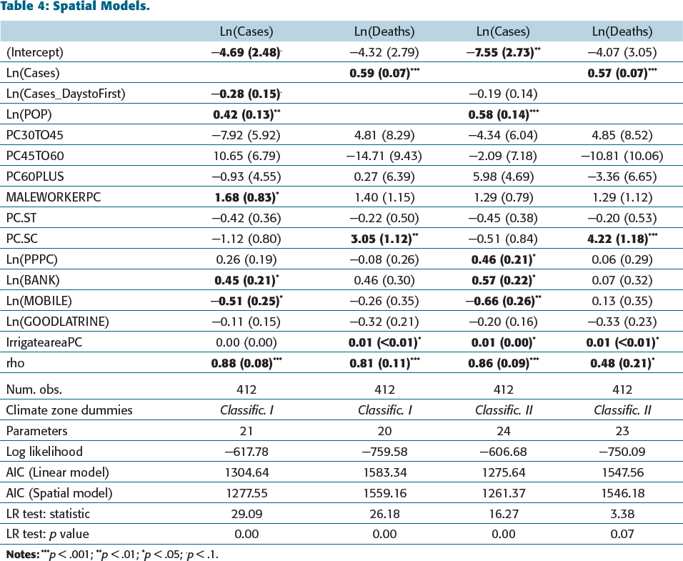
Our spatial econometric findings suggest the importance of local mobility restrictions around areas of high infection, which should diminish with distance.

CONCLUSION

The COVID-19 crisis has put economists and policymakers in a predicament. Good policy measures must be based on scientific evidence, which, although emerging, warrant increased research effort. Our study attempts to consolidate several earlier findings and explore some anecdotal conjectures related to the determinants of COVID-19 infections and deaths. We examine the association between some usual suspects: climate, demographics and socio-economic behaviour of the population. India provides an interesting setting for this study with a high degree of heterogeneity across all variables of interest: climate, demographics and socio-economic status of the population.

We examined variables with different sets of climatic controls. Although we found some evidence of different infections and death patterns across climatic zones, the patterns remain unclear. We conclude that the climatic zone controls may also be capturing geographic diversity that is correlated with the socio-economic status and behaviour of the populations. Our findings related to the association between population age groups and pandemic-related infections or deaths are not robust across model specifications.

Yet, some of our findings of regression are robust to different model specifications. For example,

A higher number of the male population and increased economic activity (e.g., banking, purchasing power, etc.) are associated with a higher number of infections.

The usage of mobile phones is associated with lower infections, possibly because they help with social distancing and contact-tracing.

Access to good latrine facilities is significantly associated with lower death rates, pointing towards the role of hygiene and social distancing.

The localities with more backward caste (SC) and agricultural population are associated with increased COVID-19-related deaths.

However, we were not able to relate population density to the impact of COVID-19. Further, spatial autoregressive models for infections and deaths indicate a significant spatial dependence on these two variables. Spatial dependence is higher in infections compared to deaths. This finding suggests the importance of including spatial dependence in regression models to capture micro-location-specific variables that are omitted from traditional regression models. More importantly, our spatial models suggest a significant role of people’s mobility in neighbouring areas in spreading the virus.

Broadly, our results portray a socio-economic picture of COVID-19-related infections and deaths. These variables are significant even after we control climatic or ethnicity-related variables. Our findings have policy implications. We find strong support for the efficacy of social-distancing-related policy measures. Results indicate that superior access to health facilities, especially in more vulnerable localities characterized by populations deprived of economic prosperity and health care infrastructure, will help control virus spread and deaths. Besides, our findings suggest that a uniform national-level policy will be ineffective, and localities must prioritize their areas of policy interventions themselves.

This study is not without its limitations. First, the infection- and death-related data must be truly representative of the reality for the policy measures based on our study to be effective. Second, our models only provide a blueprint for superior, dynamic models based on the generation and availability of regularly updated and frequent locally based data. The models can be further improved by examining the micro-data of individuals recorded at health facilities. However, our findings, especially those robust to different model specifications, provide the groundwork for further research in this area.

Footnotes

DECLARATION OF CONFLICTING INTERESTS

The authors declared no potential conflicts of interest with respect to the research, authorship and/or publication of this article.

FUNDING

The authors received no financial support for the research, authorship and/or publication of this article.

NOTES

Ashish Gupta, PhD, has worked with JLL, Bajaj Capital and Aditya Birla Capital. Presently, he is an Associate Professor at the RICS School of Built Environment, Amity University. He leads the PhD programme and research initiatives. He has written papers in reputed journals and case studies that are listed with Harvard Business Publishing and IIMA Case Centre. His research interests are land management and tenure, circular economy and net zero carbon, property valuation, development and investment risks across property types. He is a Fellow member of the Royal Institution of Chartered Surveyors (RICS) and the Indian Institute of Architects (IIA).

e-mail: agupta@ricssbe.edu.in

Prashant Das, PhD, is the Chairperson of Finance & Accounting area at the Indian Institute of Management Ahmedabad (IIMA) where he serves as an Associate Professor of Real Estate. Beyond elective courses in real estate and land, he teaches core courses in finance and accounting at IIMA. Earlier he served as an Associate Professor and the Director of Real Estate Institute at EHL Lausanne, Switzerland. He earned his PhD from Georgia State University (Atlanta USA), MS from Texas A&M University (College Station) and B.Arch, from IIT Roorkee.

e-mail: prashantd@iima.ac.in

Dongshin Kim, is an Associate Professor of Finance and Real Estate at Pepperdine Graziadio Business School, Pepperdine University. Dr Kim’s research focuses on commercial real estate, mortgages, real estate investment trusts and housing economics. He worked as a senior programming engineer at a start-up software company and is interested in technology as well. His research has appeared in premier real-estate journals. He holds a PhD in real estate, MS in real estate, MS in business administration (Finance) and BA in engineering.

e-mail: dongshin.kim@pepperdine.edu

References

Ahmadi

, Sharifi

, Dorosti

, Jafarzadeh Ghoushchi

, & Ghanbari

(2020). Investigation of effective climatology parameters on COVID-19 outbreak in Iran. The Science of the Total Environment , 729, 138705. https://doi.org/10.1016/j.scitotenv.2020.138705

Alluri

, & Nazmi

(2020). Coronavirus: What’s driving India’s 100,000 Covid-19 deaths? BBC News . https://www.bbc.com/news/world-asia-india-54352222?at_campaign=64&at_custom3=BBC+News&at_custom2=facebook_page&at_custom1=%5Bpost+type%5D&at_medium=custom7&at_custom4=F2818BD6-048D-11EB-A5E7-5C474D484DA4#:~:text

Auerbach

A. M.

, & Thachil

(2021). How does Covid-19 affect urban slums? Evidence from settlement leaders in India. World Development , 140, 105304. https://doi.org/10.1016/j.worlddev.2020.105304

BBC. (2021 May 4). India Covid: Opposition calls for full national lockdown . https://www.bbc.com/news/world-asia-india-56976214

Bhatnagar

, Mathur

, & Garg

(2019). Climate zone classification of India using new base temperature. Proceedings of the 16th IBPSA Conference (pp. 4841–4845). IBPSA Publications.

Chin

, & Lwanga

S. K.

(1991). Estimation and projection of adult AIDS cases: A simple epidemiological model. Bulletin of the World Health Organization , 69(4), 399–406.

Choudhury

S. R.

(2021 May 11). As India resists calls for a national lockdown, one economist says states should decide. CNBC . https://www.cnbc.com/2021/05/12/india-covid-economist-says-states-should-decide-on-lockdowns.html

Coşkun

, Yıldırım

, & Gündüz

(2021). The spread of COVID-19 virus through population density and wind in Turkey cities. The Science of the Total Environment , 751, 141663. https://doi.org/10.1016/j.scitotenv.2020.141663

Das

, Coulson

N. E.

, & Ziobrowski

(2019). Caste, faith, gender: Determinants of homeownership in urban India. The Journal of Real Estate Finance and Economics , 59(1), 27–55. https://doi.org/10.1007/s11146-018-9672-1

10.

Das

, Freybote

, & Blal

(2020). The importance of micro-location for pricing real estate assets: The case of hotels. Journal of Real Estate Portfolio Management , 26(1), 57–73. https://doi.org/10.1080/10835547.2020.1833612

11.

Das

, Smith

, & Gallimore

(2018). Pricing extreme attributes in commercial real estate: The case of hotel transactions. The Journal of Real Estate Finance and Economics , 57(2), 264–296. https://doi.org/10.1007/s11146-017-9621-4

12.

Engage

E. P. W.

(2021). COVID-19: Examining the impact of lockdown in India after one year. Economic & Political Weekly . https://www.epw.in/engage/article/covid-19-examining-impact-lockdown-india-after-one

13.

Ghosh

, Nundy

, Ghosh

, & Mallick

T. K.

(2020). Study of COVID-19 pandemic in London (UK) from urban context. Cities , 106(May), 102928. https://doi.org/10.1016/j.cities.2020.102928

14.

Gupta

, Banerjee

, & Das

(2020). Significance of geographical factors to the COVID-19 outbreak in India. Modeling Earth Systems and Environment , 6(4), 2645–2653. https://doi.org/10.1007/s40808-020-00838-2

15.

Hamidi

, Sabouri

, & Ewing

(2020). Does density aggravate the COVID-19 pandemic?: Early findings and lessons for planners. Journal of the American Planning Association , 86(4), 495–509. https://doi.org/10.1080/01944363.2020.1777891

16.

Handal

A. J.

, Iglesias-Ríos

, Fleming

P. J.

, Valentín-Cortés

M. A.

, & O’Neill

M. S.

(2020). ‘Essential’ but expendable: Farmworkers during the COVID-19 pandemic-the Michigan farmworker project. American Journal of Public Health , 110(12), 1760–1762. https://doi.org/10.2105/AJPH.2020.305947

17.

Holtgrave

D. R.

, Barranco

M. A.

, Tesoriero

J. M.

, Blog

D. S.

, & Rosenberg

E. S.

(2020). Assessing racial and ethnic disparities using a COVID-19 outcomes continuum for New York State. Annals of Epidemiology , 48, 9–14. https://doi.org/10.1016/j.annepidem.2020.06.010

18.

, Roberts

J. D.

, Azevedo

G. P.

, & Milner

(2020). The role of built and social environmental factors in Covid-19 transmission: A look at America’s capital city. Sustainable Cities and Society , 65(February), 102580. https://doi.org/10.1016/j.scs.2020.10258

19.

ICAR-CRIDA. (2014). District database of agricultural statistics . http://www.nicra-icar.in/nicrarevised/images/publications/DDAS

20.

Jordan

R. E.

, Adab

, & Cheng

K. K.

(2020). Covid-19: Risk factors for severe disease and death. The BMJ , 368(March). https://doi.org/10.1136/bmj.m1198

21.

Kamath

, Kamath

, & Salins

(2020). COVID-19 pandemic in India: Challenges and silver linings. Postgraduate Medical Journal , 96(1137), 422–423. https://doi.org/10.1136/postgradmedj-2020-137780

22.

Kermack

W. O.

, & Mckendrick

A. G.

(1927). A contribution to the mathematical theory of epidemics. Proceedings of the Royal Society of London. Series A, Containing Papers of a Mathematical and Physical Character , 115(772), 700–721. https://doi.org/10.1098/rspa.1927.0118

23.

Khalil

K. M.

, Abdel-Aziz

, Nazmy

T. T.

, & Salem

A.-B. M.

(2012). An agent-based modeling for pandemic influenza in Egypt. In Lu

, Jain

L. C.

, & Zhang

(Eds.), Handbook on decision making, 33 . Springer-Verlag. https://doi.org/10.1007/978-3-642-25755-1_11

24.

Khunti

, Singh

A. K.

, Pareek

, & Hanif

(2020). Is ethnicity linked to incidence or outcomes of Covid-19? BMJ , 369, m1548. https://doi.org/10.1136/bmj.m1548

25.

Kodera

, Rashed

E. A.

, & Hirata

(2020). Correlation between COVID-19 morbidity and mortality rates in Japan and local population density, temperature, and absolute humidity. International Journal of Environmental Research and Public Health , 17(15), 1–14. https://doi.org/10.3390/ijerph17155477

26.

Krishnan

(1988). Delineation of soil climatic zones of India and its application in agriculture. Fertiliser News , 33, 11–19.

27.

Kroumpouzos

, Gupta

, Jafferany

, Lotti

, Sadoughifar

, Sitkowska

, & Goldust

(2020). COVID-19: A relationship to climate and environmental conditions? Dermatologic Therapy , 33(4), e13399. https://doi.org/10.1111/dth.13399

28.

Laxminarayan

, Wahl

, Dudala

S. R.

, Gopal

, Mohan

B C.

, Neelima

, Jawahar Reddy

K. S.

, Radhakrishnan

, & Lewnard

J. A.

(2020). Epidemiology and transmission dynamics of COVID-19 in two Indian states. Science , 370(6517), 691–697. https://doi.org/10.1126/science.abd7672

29.

Liu

, Chen

, Lin

, & Han

(2020). Clinical features of COVID-19 in elderly patients: A comparison with young and middle-aged patients. The Journal of Infection , 80(6), e14–e18. https://doi.org/10.1016/j.jinf.2020.03.005

30.

Liu

(2020). Emerging study on the transmission of the Novel coronavirus (COVID-19) from urban perspective: Evidence from China. Cities , 103, 102759. https://doi.org/10.1016/j.cities.2020.102759

31.

Livingston

, & Bucher

(2020). Coronavirus disease 2019 (COVID-19) in Italy. JAMA , 323(14), 1335. https://doi.org/10.1001/jama.2020.4344

32.

Malani

, Shah

, Kang

, Lobo

G. N.

, Shastri

, Mohanan

, Jain

, Agrawal

S. T.

, Juneja

, Imad

, & Kolthur-Seetharam

(2020). Seroprevalence of SARS-CoV-2 in slums and non-slums of Mumbai, India, during June 29–July 19 , 2020. https://www.medrxiv.org/content/10.1101/2020.08.27.20182741v1

33.

Mertens

T. E.

, & Low-Beer

(1996). HIV and AIDS: Where is the epidemic going? Bulletin of the World Health Organization , 74(2), 121–129.

34.

Mishra

S. V.

, Gayen

, & Haque

S. M.

(2020a). COVID-19 and urban vulnerability in India. Habitat International , 103, 102230. https://doi.org/10.1016/j.habitatint.2020.102230

35.

Mishra

S. V.

, Haque

S. M.

, & Gayen

(2020b). COVID-19 in India transmits from the urban to the rural. The International Journal of Health Planning and Management , 35(6), 1623–1625. https://doi.org/10.1002/hpm.3047

36.

Nandi

, Balasubramanian

, & Laxminarayan

(2020). Who is at the highest risk from COVID-19. In India? Analysis of health, healthcare access, and socioeconomic indicators at the district level . https://doi.org/10.1101/2020.04.25.20079749

37.

Patel

, Shah

, & Beauregard

B. E.

(2020). Measuring multiple housing deprivations in urban India using Slum Severity Index. Habitat International, 101 . https://doi.org/10.1016/j.habitatint.2020.102190

38.

Pramanik

, Udmale

, Bisht

, Chowdhury

, Szabo

, & Pal

(2022). Climatic factors influence the spread of COVID-19 in Russia. International Journal of Environmental Health Research , 32(4), 723–737. https://doi.org/10.1080/09603123.2020.1793921

39.

Raissi

, Ramezani

, & Seshaiyer

(2019). On parameter estimation approaches for predicting disease transmission through optimization, deep learning and statistical inference methods. Letters in Biomathematics , 6(2), 1–26. https://doi.org/10.1080/23737867.2019.1676172

40.

Rashed

E. A.

, Kodera

, Gomez-Tames

, & Hirata

(2020). Influence of absolute humidity, temperature and population density on COVID-19 spread and decay durations: Multi-prefecture study in Japan. International Journal of Environmental Research and Public Health , 17(15), 1–14. https://doi.org/10.3390/ijerph17155354

41.

Resnick

, Galea

, & Sivashankar

(2020). Covid-19: The painful price of ignoring health inequities. The BMJ Opinion . https://blogs.bmj.com/bmj/2020/03/18/covid-19-the-painful-price-of-ignoring-health-inequities/

42.

Sannigrahi

, Pilla

, Basu

A. S.

, & Molter

(2020). Examining the association between socio-demographic composition and COVID-19 fatalities in the European region using spatial regression approach. Sustainable Cities and Society , 62, 102418. https://doi.org/10.1016/j.scs.2020.102418

43.

Segarra

, Jege

M. J.

, & van den Bosch

(2001). Epidemic dynamics and patterns of plant diseases. Phytopathology® . 91(10), 1001–1010. https://doi.org/10.1136/bmj.m1198

44.

Singh

K. D.

, & Gettleman

(2020). ʻRural surgeʼ propels India toward more Covid-19 infections than U.S. The New York Times . https://www.nytimes.com/2020/10/08/world/asia/india-covid-19-rural.html

45.

Sun

, Zhang

, Yang

, Wan

, & Wang

(2020). Impacts of geographic factors and population density on the COVID-19 spreading under the lockdown policies of China. The Science of the Total Environment , 746, 141347. https://doi.org/10.1016/j.scitotenv.2020.141347

46.

Tammes

(2020). Social distancing, population density, and spread of COVID-19 in England: A longitudinal study. BJGP Open , 4(3). https://doi.org/10.3399/bjgpopen20X101116

47.

Tamrakar

, Srivastava

, Parmar

M. C.

, Kumar Shukla

, Shabnam

, Boro

, Saha

, Debbarma

, & Saikia

(2020). District level correlates of COVID-19 pandemic in India. https://doi.org/10.1101/2020.10.08.20208447

48.

Tavares

F. F.

, & Betti

(2021). The pandemic of poverty, vulnerability, and COVID-19: Evidence from a fuzzy multidimensional analysis of deprivations in Brazil. World Development , 139. https://doi.org/10.1016/j.worlddev.2020.105307

49.

Thornthwaite

C. W.

, & Mather

J. R.

(1955). The water balance. Climatology , 8(1), 104.

50.

Tong

X.-J.

, Zhang

, & Wang

(2016). The cost optimal control system based on the Kermack–Mckendrick worm propagation model. Journal of Algorithms and Computational Technology , 10(2), 82–89. https://doi.org/10.1177/1748301816640704

51.

Venkateswarlu

, Raju

B. M. K.

, Rao

K. V.

, & Rama Rao

C. A.

(2014). Revisiting drought-prone districts in India. Economic & Political Weekly , 49(25), 71–75.

52.

Wan

, & Su

(2016). Neighborhood housing deprivation and public health: Theoretical linkage, empirical evidence, and implications for urban planning. Habitat International , 57, 11–23. https://doi.org/10.1016/j.habitatint.2016.06.010

53.

World Bank Group. (2020). Protecting people and economies: Integrated policy responses to COVID-19. In COVID-19 coronavirus response . World Bank. https://doi.org/10.1596/33770

54.

Yao

, Fu