Sage Journals: Discover world-class research

Abstract

The Fiscal Reform and Budget Management (FRBM) Act 2003 (and its subsequent amendments) and similar fiscal responsibility laws were legislated to rein in fiscal deficits often driven by factors other than economic imperative. This paper shows that such laws have not promoted counter-cyclical fiscal policy because of a lacuna in design, viz. measurement of fiscal deficit-as-a-share of gross domestic product (GDP). The remedy lies in targeting the cyclically adjusted fiscal deficit-as-a-share-of potential GDP instead, which correctly reflects the true fiscal position, allowing elbowroom for appropriate fiscal action for macroeconomic-stabilisation. The paper discusses ways to institutionalise the same and way forward therein.

Keywords

FRBM Fiscal Impulse Fiscal Stance Cyclically Adjusted Fiscal Deficit

Academicians and policymakers have suggested a close relook at fiscal reform and budget management (FRBM) Act on the grounds of its limited efficacy in binding the fiscal policy to achieve debt sustainability. In this context, the legislation may be viewed from a first principles approach. JM Keynes’ oft-repeated quote, ‘In the long run we are all dead. Economists set themselves too easy, too useless a task, if, in tempestuous seasons they can only tell us, that when the storm is long past, the ocean is flat again’, motivates the discussion of public finance based on various functions of fiscal policy, one of the principal ones being the ‘stability objective’. Keynes advocated counter-cyclical fiscal policy—when output falls below the economy’s potential output, the government must increase the aggregate demand to stimulate economic activity. The size of government stimulus to the economy must run in the direction opposite to the movement of aggregate economic output. Hence more government spending in periods of inadequate demand in the economy and higher taxes in the period of excess demand is prescribed.¹

Fiscal profligacy is often driven by political expediency rather than economic imperative (Srinivasa-Raghavan, 2012). So, the FRBM legislation was brought to rein in the fiscal spending to place the sovereign debt on a more salubrious path to macroeconomic stability by imposing constraints on deficit measures (typically, fiscal or revenue deficits and debt were capped at certain shares of GDP). While the impact of these bounds on government debt is discussed widely, it is worth inquiring whether the objective of counter-cyclicality in fiscal policy has been achieved.

For this purpose, we look at fiscal policy utilizing a tool used by the International Monetary Fund (IMF) called the fiscal impulse. Fiscal impulse is defined as the change in fiscal stance. The fiscal stance is the negative of fiscal balance adjusted for business cycles. A positive (negative) fiscal stance indicates that fiscal policy is expansionary (contractionary).² So, fiscal impulse points to the change in government’s fiscal stance—a positive (negative) impulse meaning a more expansionary (contractionary) fiscal stance vis-à-vis the previous fiscal. Looking at the fiscal impulse along with the output gap helps understand the conduct of the pursued fiscal policy. In any fiscal when the economy is in a boom as suggested by a positive output gap, a positive fiscal impulse reflects pro-cyclicality in fiscal policy—more expansionary when the economy is already doing well. If the fiscal impulse is negative in a period of boom, then fiscal policy is counter-cyclical—as it ought to be.

Generally, the budget can make course corrections in fiscal policy in the light of growth experience of the previous year. So, fiscal policy responds a year after the incidence of economic slowdown. Thus, we look at the output gap of the last fiscal and the current fiscal impulse (both as a percentage of potential GDP), in the post-FRBM period.

We have data for 15 years since the FRBM act was introduced. A negative fiscal impulse (a contractionary fiscal policy) co-existing with a negative output gap implies pro-cyclical fiscal conduct. The fiscal policy in India has been counter-cyclical only on four occasions since 2004–2005. Fiscal policy could not be counter-cyclical in more than 70% of the time the FRBM has operated (Figure 1).

Figure 1.

Source: Authors’ own calculations based on RBI, Budget data.

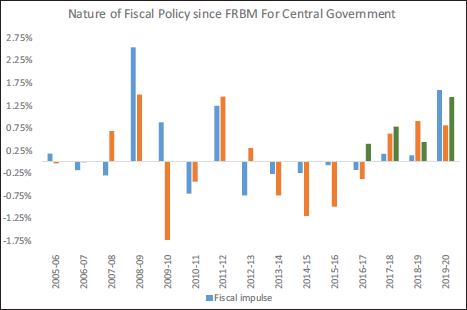
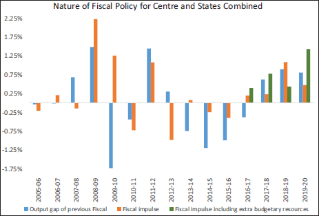
In addition, we have looked at the fiscal impulse in tandem with the output gap of previous fiscal for states as a whole and for the centre and states combined in Figures 2 and 3, respectively. As for the states, the fiscal policy was counter-cyclical in 9 of the 15 years, that is, 60% of the time, but only in 4 years for the centre and states combined. On that account, states’ fiscal policy has been more counter-cyclical than that of the centre. Since 2016–2017, expenditure financed through extra-budgetary resources also contributed to the fiscal stimulus; accounting for this does not alter our findings much. It just adds one more episode of counter-cyclical fiscal policy for central government (Figure 1).³ Notably, placing a limit on fiscal deficit-as-share of GDP ipso facto biases the fiscal policy towards pro-cyclicality: it allows a larger absolute fiscal deficit in case of a higher GDP. This is a ripe area for reform if and when we legislate a new debt-deficit law.

Figure 2.

Source: Authors’ own calculations based on RBI’s Handbook of Statistics on Indian Economy.

Figure 3.

Source: Authors’ own calculations based on RBI’s Handbook of Statistics on Indian Economy and Budget Data.

There’s a rich body of literature on institutions that enable counter-cyclicality of fiscal policy. Diallo (2009), in their study of 47 African countries for 1989–2002, uncovered a positive association between democratic institutions and counter-cyclical fiscal policies. They further elaborate their viewpoint by asserting that it is the checks and balances on incumbents that democracy entails—and not mere political competition—that helps to pursue counter-cyclical fiscal policy. They also state that democratic institutions help offset exogenous shocks that force fiscal policy into pro-cyclicality. However, this outcome is not exactly an inexorability, as several authors have pointed out that fiscal policy tends to be less counter-cyclical in developing countries than in high-income economies on account of the non-optimal efficacy of institutions (see, for example, Ilzetzki & Vegh, 2008; Kaminsky et al., 2005; Kraay & Serven, 2008). In any case, counter-cyclical fiscal policy has been advocated for wrenching languishing economies out of economic downturns rather effectively. Jha et al. (2014), in their study of 10 developing Asian economies, explored the fiscal stimuli that Asian economies administered in the wake of the 2008–2009 global financial and economic crises and attested to their role in engendering speedier and stronger recovery, with tax-based stimuli being more effective than expenditure-based ones. Thus, the quest for institutional mechanisms to facilitate counter-cyclical fiscal policy is merited. Guerguil et al. (2017) have remarked that while fiscal rules promote discipline in fiscal conduct, evidence of their impact on the cyclicality of fiscal activity is inconclusive or, in many cases, they bias fiscal policy in the direction of pro-cyclicality. Recent scholarship has pointed in the direction of certain fiscal rules having a salutary impact on counter-cyclicality. The key ingredients being flexibility (such as escape clauses), cyclically adjusted targets and a longer time horizon for complying with the fiscal rule (Guerguil et al., 2017). Specifically, budget balance rules are found to be coincident with counter-cyclical changes in overall and investment spending—more so, when public investment or other priority outlays are excluded from the scope of such rules; cyclically adjusted spending rules also yield equivalent impact; cyclically adjusted budget balance rules help to achieve counter-cyclicality in overall spending but pro-cyclicality in investment spending.

One key challenge in orienting fiscal policy towards counter-cyclicality is the all-too-well-known time inconsistency problem, in which there is a temptation to announce one policy at a point in time and be constrained to follow another later, for instance, say, because of electoral compulsions a government would be compelled to abandon running positive fiscal balance to offset deficits in the past (Taylor, 2000). Taking this into stride is desirable in designing a prudent fiscal policy rule that would be consistent in being counter-cyclical in the true sense.

There are ways to introduce counter-cyclicality into a debt law. While retaining the numerical bounds on fiscal deficit, leeway can be granted to achieve the target averaged over a couple of years instead of each year individually. This takes care of the time-inconsistency question by allowing an incumbent government desirable flexibility in adhering to fiscal discipline (and therefore, debt targeting) while supporting counter-cyclical fiscal action. If the time horizon so involved coincides with the period a government typically remains in office, this would be a splendid way of finding consonance between business and electoral cycles. Alternatively, provision can be made to modulate expenditure growth such that the constituent components coupled with their multiplier values cumulatively close the output gap in the economy. Some authors have also suggested moving from the prevalent annual budgeting convention to a multi-year budgeting practice, since keeping headline fiscal deficit under check cannot be achieved without resorting to pro-cyclical fiscal measures. Hou (2006) describes the practice of governments first committing themselves to numerical bounds on fiscal deficits but subsequently amending their pledges to permit a more flexible attitude towards achieving such goals as an ad hoc manner of dealing with the unavoidable pro-cyclicality that such fiscal discipline entails. Thus, an argument is made favouring balancing the budget over a business cycle instead of the usual fiscal year horizon. In this context, there seems to be a preference for a budget stabilization fund (BSF), which is an earmarked fund with regular flows into its corpus and upon which withdrawals are legally forbidden except in budgetary shortfalls. It has been empirically proven that for the period 1979–1999, BSFs helped the 50 states of USA pursue an effective counter-cyclical strategy during periods of three national recessions and numerous regional downturns (Hou, 2006). On a related note, the idea of a similar fund has been mooted from time to time in the Indian context (Gopinath, 2009; Thorat & Roy, 2001).

On a separate, though related footing, if a cyclically adjusted fiscal deficit (CAFD) as a share of potential GDP is used as a metric for fiscal planning, then the fiscal policy becomes better reflective of the business cycle than a headline fiscal deficit (FD) number as a share of actual GDP otherwise captures. By appropriately adjusting the revenues and expenditures with a factor linked to the output gap (see note 3 for an elaboration)—more precisely, by depressing the headline fiscal deficit number in the event of a positive output gap and inflating it in case of a negative output gap—it provides for greater elbowroom for fiscal authorities for fiscal activism in case of the latter. When in addition, the actual output is at full capacity, as is the case when growth has stabilized at some stationary level, the cyclically adjusted fiscal deficit also stabilizes as a proportion to GDP, robbing fiscal policy of much of its discretionary imperatives. However, discretion returns when output falls below full capacity (as had happened during COVID-19 situation, for instance). The discretion is about how large the fiscal deficit should be, considering the potential impact of higher government spending on inflation, possible crowding out of private investment and likely excessive stress on balance of payments (BOP).

When we target CAFD as a share of potential GDP as the fiscal metric in our fiscal law, we remedy the shortcoming that placing a limit on fiscal deficit-as-share of GDP ipso facto biases the fiscal policy towards pro-cyclicality by allowing a larger absolute fiscal deficit in case of a higher GDP. Let us understand this by seeing an illustration.

Illustration: To motivate the preceding argument, let us consider some numbers. Say, potential output in an economy is 1,000, the government collects tax revenues of 300 and spends 500. We consider the baseline scenario where output equals the potential and visualize the outcomes on fiscal-deficit-as-a-proportion of output and cyclically adjusted fiscal deficit as a proportion of potential output under alternative levels of actual output.

Variable/scenario	Y	Yp	T	G	FD/Y	CAFD/Yp
Baseline	1,000	1,000	300	500	–0.2	–0.2
Alternative 1 (Bust)	800	1,000	300	500	–0.25	–0.125
Alternative 2 (Bust)	500	1,000	300	500	–0.4	0.1
Alternative 3 (Boom)	1,250	1,000	300	500	–0.16	–0.26
Alternative 4 (Boom)	1,500	1,000	300	500	–0.13	–0.3

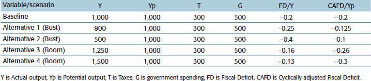
Y is Actual output, Yp is Potential output, T is Taxes, G is government spending, FD is Fiscal Deficit, CAFD is Cyclically adjusted Fiscal Deficit.

In the above illustration, ceteris paribus would mean that, potential output, government revenues and expenditure would remain constant. Under the baseline scenario, when actual output is equal to the potential level, fiscal deficit, as well as CAFD, is at 20% of the output. In the periods of bust, as in alternatives 1 and 2, FD to output worsens—simply because the denominator is smaller with the numerator remaining unchanged. If a fiscal law targets fiscal deficit to GDP ratio, it is quite visible that fiscal authorities would face constraints in being fiscally active precisely at a time when it is essential. However, if they were to be targeting the CAFD as a share of the potential output, we see that as the negative output gap rises the scope for them to administer fiscal stimulus increases as the output gap rises. Equivalently, the fiscal deficit as a share of GDP improves in case of a positive output gap, giving off a sense of comfort for fiscal authorities. The CAFD, as a proportion of potential output, instead rightly recognizes the purely arithmetic reasons that drive it and suggests fiscal prudence during economic prosperity.

This is as far as positive economics shall remark about India’s fiscal law. As argued earlier, there has been a case made out for pursuing a counter-cyclical fiscal policy for better realization of the macroeconomic stabilization objective of Keynes. Normatively speaking, therefore, fiscal policy conduct can then be oriented along counter-cyclical lines. Because the fiscal authorities would no longer be stymied by a headline FD as a share of GDP, fiscal intervention can be suitably tailored to be expansionary (i.e., a positive fiscal impulse) as a follow-up to a negative output gap. If a coveted level of full-employment level of fiscal deficit (whereupon, CAFD and FD will be identical) is arrived at—say, 3% of GDP—the debt law may provide for raising the size of the fiscal deficit to address the negative output gap in the economy. Some provision can be made to modulate the growth of expenditure such that the constituent components, coupled with their multiplier values, cumulatively close the economy’s output gap. Equivalently, the size of the fiscal deficit allowed under the law may be raised by the magnitude required to bridge the output gap. (For example, in alternative scenario 1 in the illustration above, the negative output gap is 1.25, that is, potential output is 25% higher than actual output. In such a case, the fiscal deficit may be allowed to go up by that quantity such that taking into account the multiplier associated with the components of expanded expenditure, a cumulative rise in fiscal deficit closes the negative output gap of 1.25.) The size of this discretionary intervention must be prudently sized based on the coveted need to allow the private sector the due laissez-faire economic space and the probable spillover of excessive fiscal intervention.

There are sophisticated techniques for estimating cyclically adjusted fiscal deficit.⁴ However, these techniques may not be relevant as, operationally, budget staff would want to project cyclically adjusted fiscal deficit in the year ahead so that an expenditure envelope could be arrived at. For this purpose, the GDP level—and not growth—needs to be estimated for the budget year, so that its shortfall from potential GDP level can be estimated in value and not growth terms. Growth may give a misleading picture because of base effects when a high GDP growth rate may be estimated on a low base emerging from the impact of an economic shock giving an illusionary impression that all is well with the economy. In contrast, in reality, the shortfall of actual output vis-a-vis its potential may continue to prevail. This shortfall is reason enough to plan for an expansionary fiscal policy, and the element of discretion is the size of the expansion.⁵ In general, fiscal expansion should be smaller the closer the economy is to the potential output so that the private sector gets a larger space in the economy as it should be. Fiscal discipline becomes paramount the closer the economy is to its potential as an expansionary fiscal stimulus at this stage bears the seeds of high inflation while potentially leading to crowding out of private investment and excessive stress on the BOP.

To facilitate this, estimates of potential output should be updated annually, and its estimate should be made increasingly sophisticated by developing a more comprehensive and granular database. A more precise estimation of the future output would allow its comparison with the potential output, facilitating the desired programming of expenditure and revenue actions—to fulfil the stabilization function while adhering to fundamental canons of public economics. The need of the hour is to expand and keep upgrading the skill base and technical wherewithal in the budgeting wing.

The idea of cyclical adjustment of fiscal variables is not exactly novel. Advanced economies such as Canada, New Zealand, the United Kingdom, the United States, and so on, not only compute cyclically adjusted fiscal balances but some countries explicitly factor them in fiscal laws to impart counter-cyclicality to fiscal policy conduct (Pradhan, 2019). The approaches preferred by these advanced countries are broadly similar and rely on the production function approach to estimating potential output (CBO, 2004; Jacob & Robinson, 2019; OBR, 2011; PBO, 2018).⁶ In the UK, in particular, they estimate potential output and the associated output gap in nine ways to inform their judgment (OBR, 2011). Pradhan (2019) calculates the potential output for India at the national and sub-national levels and discusses that potential output estimation through the use of the production function approach at the states’ level is stymied by the non-availability of state-wise data on net capital stock; more generally, the assumptions concerning functional form and shares of capital and labour account for the uneasiness about the credibility of the estimated potential GDP and output gap.

Admittedly, there are constraints in being able to implement counter-cyclical fiscal policy when one does not have a firm grip on the GDP figure of the fiscal year ahead and the potential GDP. Estimation of potential GDP, regardless of the technique adopted, has some shortcomings: one, it is based on some statistical relationships and, to that extent, involves an aspect of randomness; two, most methods suffer from an end-of-sample bias, thereby rendering estimates particularly uncertain for the most recent period; three, economic data pertaining to recent history are subject to maximum revisions, with a knock-on effect on the precision of estimates (CBO, 2004). Also, counter-cyclical fiscal intervention must be pursued in consonance with ensuring debt-sustainability. These issues aside, there is no countervailing thought to the imperative of baking counter-cyclicality of fiscal policy into our debt-deficit law. As a precursor to this ultimate destination, there is a pressing need to institutionalize the estimation of potential GDP and the output gap in the Ministry of Finance in the Government of India, subsequently allowing for the diffusion of this coveted practice across state governments.

Footnotes

ACKNOWLEDGEMENT

All views are personal. Part of the motivation for this article is attributed to an interaction of one of the authors with Dr Michael D. Patra, Deputy Governor of the Reserve Bank of India. The authors are thankful to Dr Sitikantha Patnaik, Dr Sangita Misra, Bhanu Pratap of the Reserve Bank of India, Professor Arup Mitra of the Institute of Economic Growth, Dr Jai Chander of the Central Bank of Oman and Dr Arunish Chawla of the IMF for their helpful comments on an earlier version of the article.

DECLARATION OF CONFLICTING INTERESTS

The authors declared no potential conflicts of interest with respect to the research, authorship and/or publication of this article.

FUNDING

The authors received no financial support for the research, authorship and/or publication of this article.

Notes

Anshuman Kamila is Assistant Director (Officer Trainee of the Indian Economic Service), Department of Economic Affairs, Ministry of Finance. He holds a post-graduate and an MPhil degree in Economics. He has worked in the Department of Economic and Policy Research of the Reserve Bank of India. He takes an interest in fiscal issues.

e-mail: kamila.anshuman@gov.in

Ritika Bansal is Assistant Director (Officer Trainee of the Indian Economic Service), Department of Economic Affairs, Ministry of Finance. She holds a post-graduate degree in Economics. She has taught economics at the post-graduate and undergraduate levels and worked in the Department of Commerce, Ministry of Commerce and Industry as a research associate.

e-mail: ritika.bansal@gov.in

Rajiv Mishra is an Economic Adviser, Department of Economic Affairs, Ministry of Finance. He is a macroeconomist and does growth diagnostics for the government. His background in preparing government budgets has given him insights into addressing fiscal challenges.

e-mail: r.mishra67@gov.in

References

Congressional Budget Office (CBO). (2004). A summary of alternative methods for estimating potential GDP . The Congress of The United States

Diallo

(2009). Tortuous road toward counter-cyclical fiscal policy: Lessons from democratised sub-Saharan Africa. Journal of Policy Modelling , 31, 36–50.

Gopinath

(2009). Sub-national fiscal reforms and debt management—Indian experience [Paper Presentation]. Workshop on ‘Sub-national Fiscal Reform and Debt Management’, Washington, Economic Policy and Debt Department, World Bank, April 29, 2009.

Guerguil

, Mandon

, & Tapsoba

(2017). Flexible fiscal rules and counter-cyclical fiscal policy. Journal of Macroeconomics , 52, 189–200.

Hou

(2006). Budgeting for fiscal stability over the business cycle: A counter-cyclical fiscal policy and the multiyear perspective on budgeting. Public Administration Review , 66(5), 730–741

Ilzetzki

, & Végh

C. A.

(2008). Procyclical fiscal policy in developing countries: Truth or fiction? [Working Paper No. 14191]. NBER.

Jacob

, & Robinson

(2019). Augmenting the Reserve Bank’s output gap indicator suite [Analytical Note Series AN2019/08]. Reserve Bank of New Zealand.

Jha

, Mallick

S. M.

, Park

, & Quising

P. F.

(2014). Effectiveness of counter-cyclical fiscal policy: Evidence from developing Asia. Journal of Macroeconomics , 40, 82–98

Kaminsky

, Reinhart

, & Vegh

(2005). When it rains, it pours: Procyclical capital flows and macroeconomic policies. In Gertler

, & Rogoff

(Eds.), NBER Macroeconomics Annual 2004 (pp. 11–53). MIT Press.

10.

Kraay

, & Servén

(2008). Fiscal policy responses to the current financial crisis: Issues for developing countries (Research Brief) . World Bank.

11.

Office for Budget Responsibility (OBR) (2011). Estimating the output gap (Briefing Paper No. 2). Office for Budget Responsibility, U.K.

12.

Parliamentary Budget Office (PBO). (2018). PBO’s approach to measuring potential GDP . Office of The Parliamentary Budget Officer, Canada.

13.

Pradhan

B. K.

(2019). Cyclically adjusted primary balance for centre and states in India . Development Planning Centre, Institute of Economic Growth. http://fincomindia.nic.in/writereaddata/html_en_files/fincom15/StudyReports/Cyclically%20adjusted%20primary%20balance%20for%20Centre%20and%20States%20in%20India.pdf

14.

Ramachandran

(2001). Dynamics of inflation and fiscal deficits: Implications for inflation targeting. Journal of Indian School of Political Economy , 3(13).

15.

Srinivasa-Raghavan

T. C. A.

(2012). On the turnpike: Indian economy since 1947 & Indian economic service at 50 . Academic Foundation

16.

Taylor

J. B.

(2000). Reassessing discretionary fiscal policy. Journal of Economic Perspectives , 14(3, 21–36.

17.

Thorat

, & Roy

(2001). Contingent liabilities at the state level—The Indian experience [Paper Presentation]. World Bank Conference Fiscal on Policies to Accelerate Economic Growth, New Delhi, May 21–22, 2001.

A Reformist Thought to Fiscal Reform and Budget Management