
Abstract
When considering multiphase flow scenarios, the interpretation of petrophysical properties poses significant challenges for production forecasts and reservoir modeling. The findings of the numerical modeling were therefore subject to uncertainty because characteristics like relative permeability and capillary pressure curve were hardly ever bound by interpretations. The uncertainty may result in inaccurate predictions of reservoir performance and skewed perceptions of the reservoir. Due to the difficulty in directly interpreting such property from the available field data and the expensive cost of coring, analyses or experimental measurements to determine relative permeability and capillary pressure were infrequently carried out. Such a gap would be filled by a straightforward yet rigorous method. In this study, we develop production projections for a wide range of three-phase compositional volatile oil reservoirs. Then, we used an artificial neural network to figure out how petrophysical characteristics and production data relate to one another. The artificial neural network model was adjusted, and the final trained model was tested blindly to determine how well it predicted permeability, multiphase relative permeability, and capillary pressure data. For the testing scenarios, consistency is seen between the predicted values and the original ones, despite some mispredictions being present. To provide production projections that can be compared to those from the reservoir model that include the initial petrophysical characteristic, the anticipated properties are then propagated into reservoir models. The comparison findings show that for 65/59/34 out of 74 testing scenarios, the reservoir model with artificial neural network-predicted features can anticipate oil/gas/water output with < 20% inaccuracy. With the developed artificial neural network tool, the reservoir engineers can evaluate the three-phase relative permeability surface from rate-transient data conveniently improving the accuracy of the relative permeability data implemented by history matching or from core experiments which sometimes are extremely expensive. The findings of this study can help for a better understanding of the relationships between three-phase rate-transient data and the relative permeability surface as well as the horizontal/vertical permeability.
Introduction
The great majority of reservoir simulations in the industry employ relative permeability, capillary pressure, and permeability. The ratio of effective permeability to absolute permeability is known as relative permeability. Relative permeability, whose property profile considerably alters production performance, strongly influences reservoir flow behavior. In the simulation study for reservoirs, relative permeability has been employed as a key history-matching parameter, but it is rarely restricted by observed or forecasted data.
If erroneous relative permeability statistics are employed, false reservoir performance may be anticipated. The length of transition zones, on the other hand, could fluctuate due to a capillary pressure profile, resulting in various flow patterns and an early or late water or gas breakthrough into the well. If the improper capillary pressure relationship is used, it might potentially misrepresent the flow regime in the vertical direction. Relative permeability, capillary pressure, permeability, and porosity, if inaccurately evaluated, cause biased production predictions and encourage poor development choices. The use of petrophysical characteristics in enhanced oil recovery (EOR) projects is a notable example because multi-phase behavior in EOR projects heavily depends on relative permeability. An EOR project could be harmed by an inaccurate depiction of relative permeability. In reservoir engineering projects like reservoir development plans, enhanced oil recovery, and carbon dioxide sequestration, permeability is crucial. Since it can typically be calculated from well testing and rate-transient analysis, permeability is less ambiguous. However, a reservoir model for an oil field is also prone to erroneous estimation of permeability. It must therefore be restrained using efficient techniques. Even when coring is an option, the cost of the coring procedure itself is considerable, which raises the price of reservoir characterization and the price of the development plan. Due to the high overhead, coring in offshore operations is considerably more expensive, costing up to $500,000 for each operation.
The relative permeability of the sample can be estimated using two traditional methods: the steady-state technique and the unsteady-state method. One way to calculate three-phase relative permeability is to assess the two-phase flow's relative permeability separately and couple it using Stone's models I (1970) and II (1973). The flow rates and pressure drop between the two core ends are measured to determine the two-phase relative permeabilities. The relative permeability of the phases is then determined by applying Darcy's law to the effective permeability of each phase. The relative permeability curve for a given system's one-direction saturation change typically requires 50–100 measurements (Sarma et al., 1994). An issue with the steady-state technique is that capillary pressure is believed to be zero. The steady-state technique does not take into consideration the “end effects,” or the consequences of the capillary force discontinuity at the end of the flow.
Another problem is that the fluids may interact with the sample because of the enormous injection volume and lengthy experimentation period, which has an impact on how accurate the results of the experiment are.
When employing the steady-state methods to measure the relative permeability curve, gravitational force is another aspect to take into account. If the viscous force is negligible relative to the capillary force and gravity force in the reservoir, the intermediate region and the section furthest from the endpoints may be meaningless. The relative permeability curve of the two-phase flow can also be estimated using the unsteady-state approach. Numerous tests have been performed using techniques created around this concept. Such studies include the following: Goodfield et al., 2001; Helset et al., 1998; Islam and Bentsen, 1986; Johnson et al., 1959; Jones and Roszelle, 1978; Kalbus and Christiansen, 1995; Marle, 1981; Ruth et al., 1988; Sigmund and McCaffery, 1979; Siddiqui et al., 1998; Toth et al., 2001, and Welge, 1952. Johnson et al. (1959) developed a displacement test to estimate the relative permeability of reservoir formation. Welge (1952) developed a method to evaluate the average saturation during the unsteady-state method to improve the unsteady-state relative permeability measurements. Jones and Roszelle (1978) demonstrated graphical constructions that simplify the calculation of relative permeability from displacement data. Sigmund and McCaffery, (1979) improved the unsteady state measurement method for determining the heterogeneous porous media's relative permeability. Marle (1981) proposed an unsteady-state measurement method. Ruth et al. (1988) improved the Welge method (1952) by incorporating explicit relative permeability function forms and did sensitivity analysis. Toth et al. (2001) developed an unsteady-state method for two-phase fluid injection settings during relative permeability measurements. Islam and Bentsen (1986) used the microwave attenuation technique to develop an unsteady-state measurement method. Kalbus and Christiansen (1995) improved the Johnson–Bossler–Naumann (JBN) method and the Hagoort method. Helset et al. (1998) developed a method to measure the relative permeability at all saturation with the experiments carried out at low injection speed, in contrast to high speed in most methods. Siddiqui et al. (1998) developed an unsteady-state method for evaluating three-phase relative permeability under a three-phase flow path. Goodfield et al. (2001) extended previously published techniques for interpreting gravity drainage floods by including viscous and capillary forces and calculating relative permeabilities directly from in-situ saturation and pressure drop data, without the need to use simulation methods.
The saturated core of the unsteady-state technique is injected with a phase. The pressure across the core and the flow rate of each phase are then monitored. The calculations are made using the results and the standard Buckley–Leverett theory (Buckley and Leverett, 1942). The homogenous assumption and one-dimensional assumption that underpin this family of techniques are flaws. The JBN approach was discovered to have substantial inaccuracy when converting average injectivity into a point value (Johnson et al., 1959). When employing Jones and Roszelle's approach or JBN method, the differentiation and breakthrough point estimation are the additional sources of mistakes. Additionally, Heaviside and Black (1983) and Crotti and Rosbaco (1998) identified the following issues: the relative permeability measured by running experiments at various rates and lengths may vary; the endpoint relative permeability is affected by mobility ratio; additionally, the capillary and gravity effects are not taken into account in the unsteady-state method. The data near the endpoint are calculated. As shown by earlier investigations, two-phase relative permeability can also be calculated from capillary pressure data (Brooks and Corey, 1966; Purcell, 1949). This method is helpful for samples with unique fluids or low permeability samples. The category also includes samples of insufficient size that can be used for capillary pressure measurement but cannot be utilized for flow tests (Sahimi, 2011). Li and Horne (2002) have demonstrated that the relative permeability determined from capillary pressure is accurate. Based on a variety of petrophysical and fluid parameters, Guler et al. (2003) make predictions about the relative permeability. By using this approach, the time-consuming laboratory experiment used to determine relative permeability is avoided. However, because their approach needs residual saturation, it is still reliant on core-based experiments for its measurements. Additionally, rather than predicting a relative permeability profile, the tool forecasts single-value relative permeability. For both oil–water and oil–gas systems, Silpngarmlers et al. (2002) developed artificial neural networks (ANNs) to forecast relative permeability using petrophysical and fluid properties. However, their approach still only yields a single-value prediction.
To forecast relative permeability in massive carbonate reservoirs, Al-Fattah and Al-Naim (2009) constructed ANN models. However, their approach still needs petrophysical inputs like irreducible saturations and residual saturation. It is more difficult to measure three-phase relative permeability than two-phase ones. Methods for linking two-phase relative permeability with two-phase relative permeability were also created due to the incredibly high time cost and experimental complexity. These techniques include Stone's Model I and Stone's Model II, as well as the Hustad–Holt correlation (1992). Mercury injection or a centrifuge can be used to measure capillary pressure curves. The resulting capillary pressure is then translated to capillary pressure data for the chosen liquid–gas and water–oil systems with Leverett J-function assistance. Cores and experimental operations are needed for all of the approaches outlined above. Coring is a pricey operation that is hardly used for wells. Due to the high operation costs, offshore coring is particularly expensive, costing up to $500,000. The petrophysical qualities take time to measure and might be challenging at times.
In this study, our goal is to use production data to assess permeability, capillary pressure curves, and three-phase relative permeability properties. The evaluation of reserve and hydraulic fracture qualities has mostly relied on production data (Blasingame et al., 1991; Fetkovich, 1980; Wattenbarger et al., 1998; Zhang and Ayala H., 2016, 2017, 2018). Using proxies, Zhang and Ertekin (2021) evaluated the petrophysical characteristics of black oil reservoirs. To the best of our knowledge, it has not yet been employed to calculate the relative permeability and capillary pressure for compositional volatile oil reserves.
The key difference between this specific study and previous studies from different genres is that we utilize rate-transient data to directly evaluate the three-phase relative permeability relationship in terms of relative permeability curves in the framework of Stone's Model II while the previous method either relies on core experiments and measurements or predict single-point two-phase relative permeability given other petrophysical properties which has no production data involved. By not using core-related data we are able to save thousands of to millions of dollars in predicting relative permeability curves and surface petrophysical properties and this also avoided the shortcoming of predicting only single-point two-phase water–oil or oil–gas relative permeability data using traditional previously developed artificial neural network tool, which takes tens of trials to predict complete relative permeability curves which are not applicable to three-phase reservoir water, oil and gas fluid flow in porous media. It should be noted that this study can be extended to the hydrogen production scenario and CCUS scenario considering previous studies (Sun et al., 2020, 2022, 2023).
By utilizing the ANN, a general functional relationship capturer, in this study, we can estimate three-phase relative permeability features, capillary pressure curves, and permeability for volatile oil reservoirs. A scheme of the ANN in this study is presented in Figure 1.
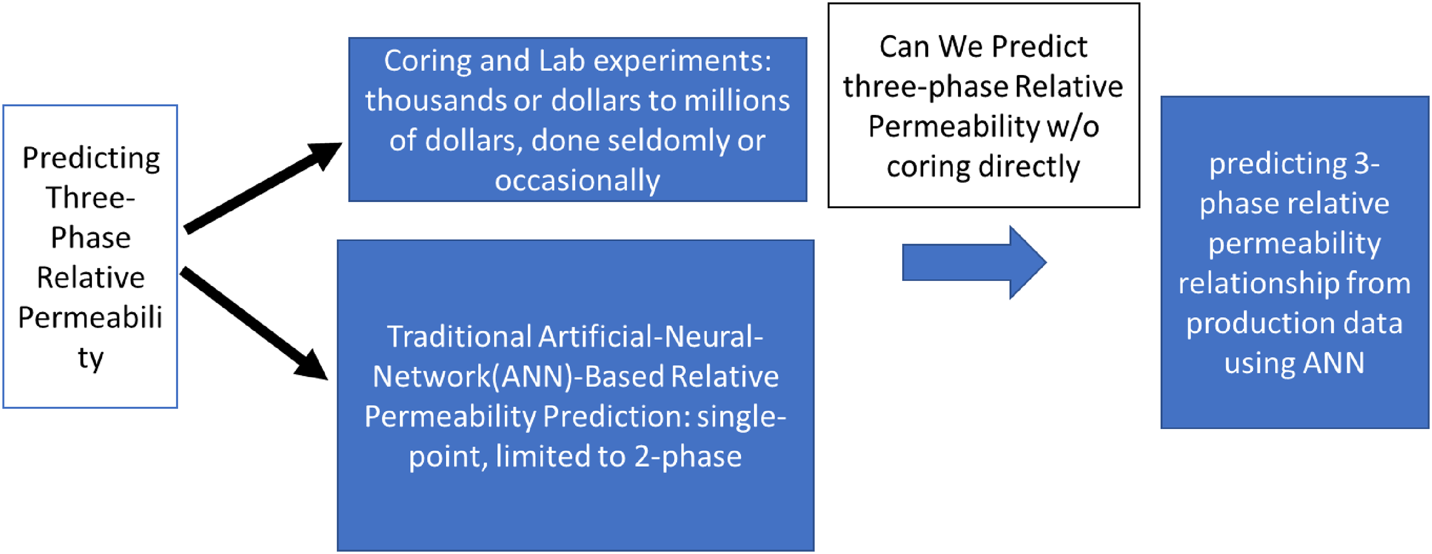
Schematic diagram of the problem in this study.
Methodology
Artificial neural network
An excellent tool for time-series prediction, grouping, pattern recognition, and other tasks is the ANN. It has been utilized as a function approximator for demanding complex numerical computations in various areas of the oil and gas industry, such as reservoir simulations, phase behavior calculations, seismic wave interpretation, etc. Instead of taking hours or days to estimate reservoir production behavior using reservoir simulations, ANNs can do so in just a few seconds. With many inputs, an ANN may successfully mimic any function, as demonstrated by Hornik et al. (1989). An ANN can imitate several outputs. Based on the neural networks in the brain, ANN is proposed. Over the past 70 years, its theory has undergone dramatic change. It is currently one of the most effective techniques for time-series prediction, clustering, decision-making, pattern identification, etc. Over the past 20 years, the use of ANN has been the subject of a substantial amount of study in the petroleum and natural gas fields. For instance, Gorucu et al. (2005) developed ANNs to predict the performance of enhanced coalbed methane and CO2 sequestration projects. Olufemi et al. (2004) developed ANNs for performance prediction and screening of carbon dioxide sequestration in coal seams. Ayala and Ertekin (2007) and Ayala et al. (2007) built ANNs to analyze gas-cycling performance and studied development in gas/condensate reservoirs. There are numerous further uses (Alajmi and Ertekin, 2007; Artun et al., 2011a, 2011b; Bansal et al., 2013; Enab and Ertekin, 2014; Enyioha and Ertekin, 2014; Parada and Ertekin, 2012; Ramgulam et al., 2007; Siripatrachai et al., 2014; Sun and Ertekin, 2012, 2017, 2018). Such work also includes Masoudi et al. (2012) and Masoudi et al. (2014).
Because of its distinctive structure, ANN can simulate relationships. The human brain contains 100 billion neurons. The neurons are interconnected to enable a variety of all-encompassing tasks. The details of neurons can be found by Zhang and Ertekin (2021).
By mimicking a neuron's structure, an artificial neuron can be produced. The first part of Figure 2 shows a visual representation of a synthetic neuron. On the diagram, you can see the input from earlier neurons (P1 to Pn), weights related to each input (W1 to Wn), a bias (b), a processing function (f), and output (a). The bias, weights, and inputs are used to evaluate a contain-it-all input value. The processing function gets the input and uses it to produce an output after passing it along. The feedforward network is one of the most often utilized networks. Neurons are organized into layers. All of the neurons in the two levels are connected to form crosslinks between adjacent layers. Each link has a unique weight attached to it. As previously described for a single neuron, each neuron in a layer operates similarly. The type of transfer function that is used can differ from layer to layer, changing how an artificial neuron layer reacts to input from a lower layer. The second part of Figure 2 shows a two-hidden-layer feedforward ANN. The ANN is shown as a training dataset. Calculated and compared with the accurate output is the error of the output of the ANN. To transmit the error back to the input, a backpropagation method is used. Backpropagation occurs from the output layer to the input layer. The gradient descent algorithm, conjugate gradient method, quasi-newton algorithm, and Levenberg–Marquardt algorithm are common backpropagation algorithms.
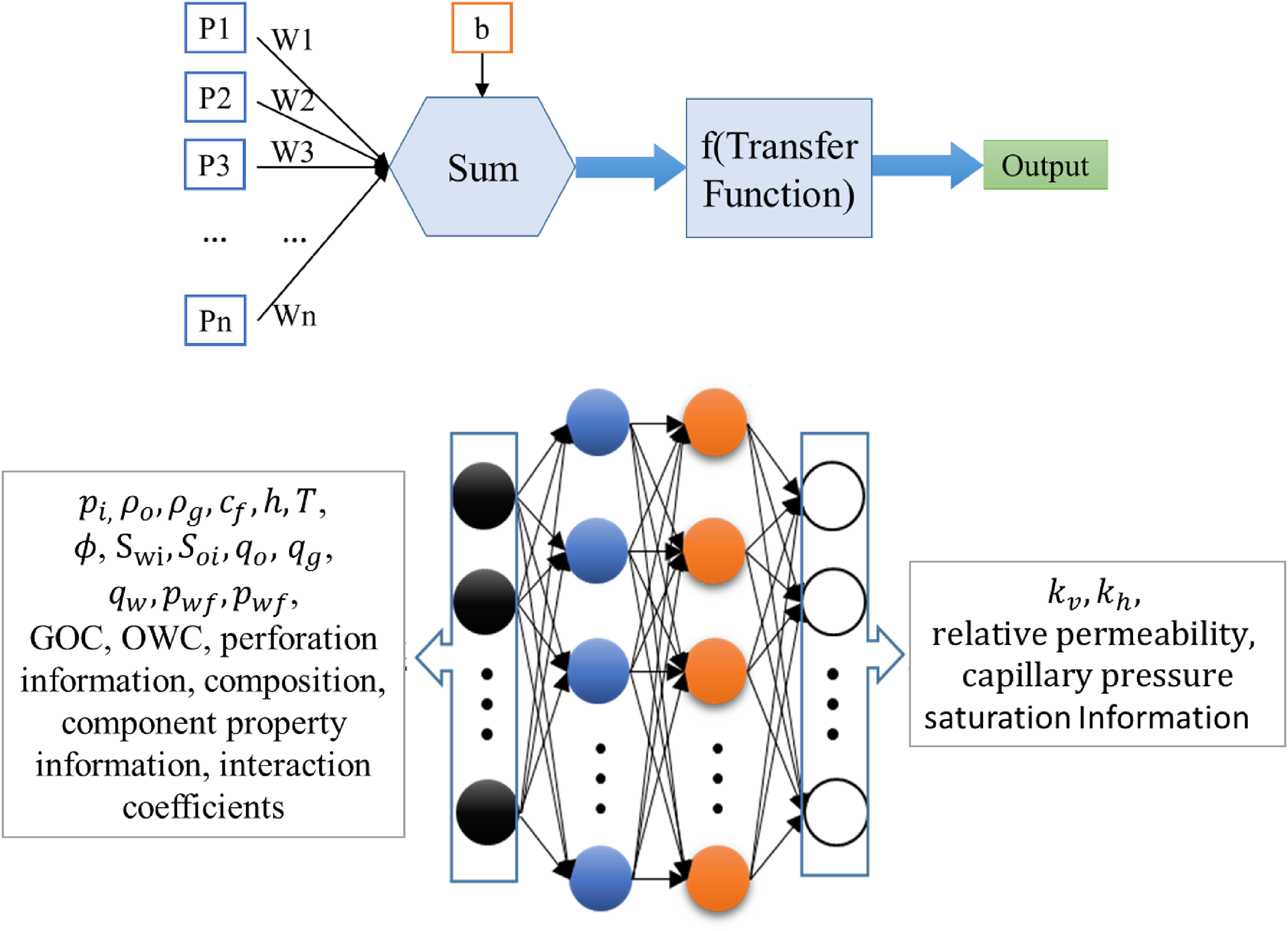
Illustration of an artificial neuron (Zhang and Ertekin, 2021) and a feedforward network with two hidden layers.
Several variables, including data structure, transfer function type, number of neurons, number of layers, error function, and training function, all have an impact on an ANN's capacity to forecast, specifically on how well the relationship capture process works. Different kinds of ANNs are suitable for various kinds of application circumstances that involve different numbers and organization of input and output parameters. Complex functional interactions typically require more layers and neurons than simple ones. A variety of structures are developed for training to increase the likelihood of finding the ideal ANN structure.
Determination of ANN structure
The feedforward neural network is fully connected between layers and they are only connected between two closely located layers. The number of input neurons is determined by the number of time points that are contained in a production rate time series. It is also determined by the number of other data. The number of hidden layers and the number of neurons in each hidden layer are randomly chosen so that the structure of the feedforward network is to a large extent various. During the creation phase, ANN configurations are altered at random. The number of layers is chosen at random from 1 to 6. Between 1 and 600 neurons are randomly produced for each layer. The reason why six layers are used is that the computation cost of ANN when the number of layers is more than six is high and it incurs additional cost to the training. Another reason is it is rarely seen in previous oil and natural gas engineering applications of feedforward network construction that the number of layers needs to be larger than six. Also, the number of neurons maximum does not exceed 600 because assigning more than 600 neurons in this case simply elevates computational cost, and this 600 plus number of neurons is rarely seen in previous oil and natural gas engineering artificial neural network construction in the authors’ experiences. The reason the upper limit is so high is that the number of inputs is high and there are 442 neurons to take in all parameters as input. The number of layers is more than the number of layers typically used considering that one to two layers is a subset of one to six layers. Also, we do this in case more than two layers are needed. The number of neurons is much larger than the typically adopted number of neurons (15–30) just in case more neurons are needed to produce a stronger-performing artificial neural network. However, it is realized that this number of layers and such a large number of neurons are not necessary and could be reduced one. The log-sigmoid transfer function, hyperbolic tangent sigmoid transfer function, radial transfer function, saturating linear transfer function, and symmetric saturating linear transfer function are all possible candidates for the transfer function for each layer. Each ANN receives one of the following training functions at random: gradient descent, one-step secant, Powell–Beale conjugate gradient, and Polak–Ribiere conjugate gradient. Each structure receives a maximum of 500 epochs of training. Equation (1) serves as the performance function in our study.

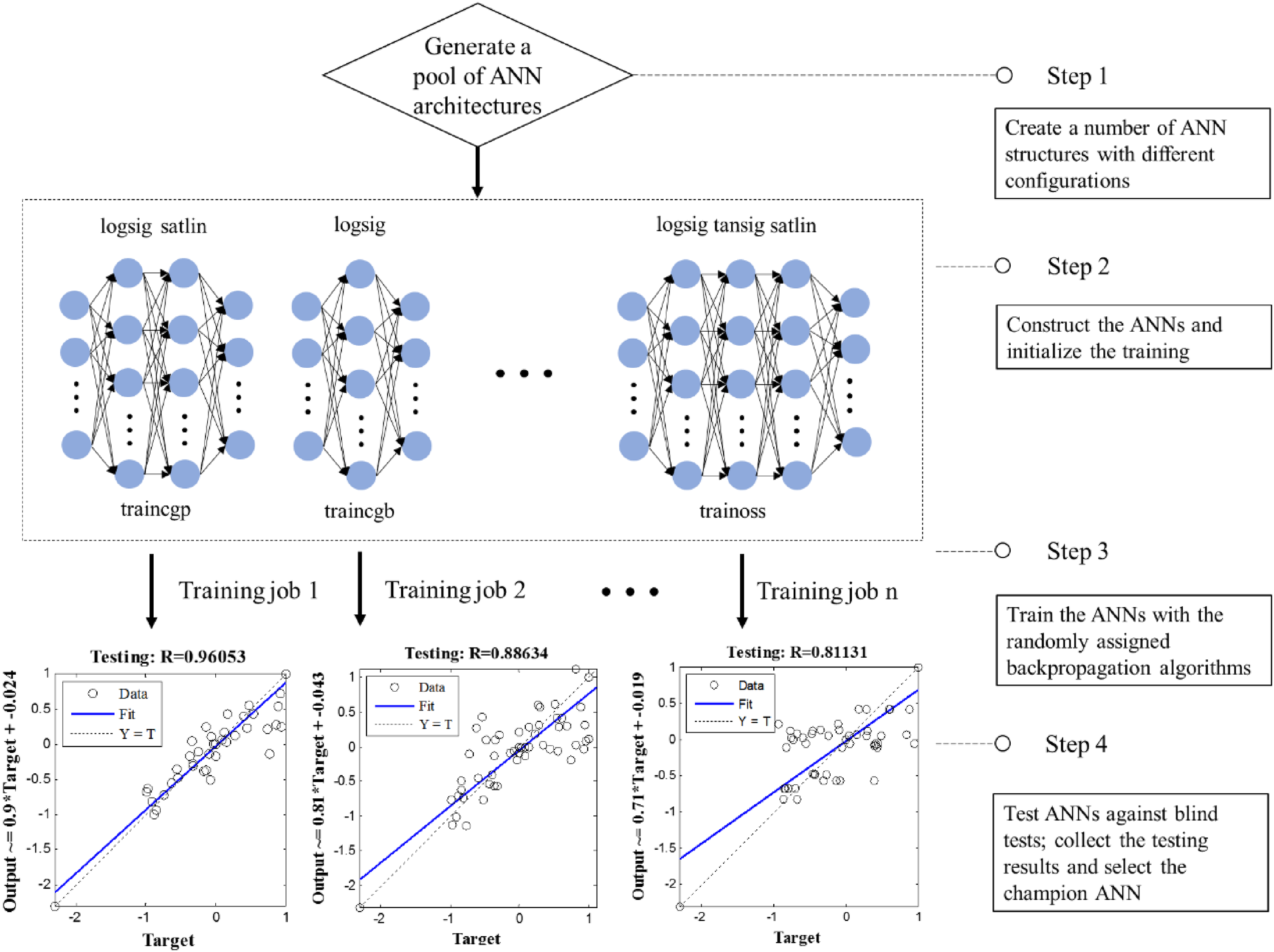
Artificial neural network (ANN) optimization and training workflow.
Where logsig is log-sigmoid transfer function; satlin is saturated linear transfer function; tansig is hyperbolic tangent sigmoid transfer function; traincgp is conjugate gradient backpropagation algorithm with Polak–Ribière updates; traincgb is conjugate gradient backpropagation algorithm with Powell–Beale restarts; trainoss is one-step secant backpropagation algorithm.
ANN development workflow
A volatile oil reservoir contains lighter hydrocarbon than black oil and is also generally lighter in terms of density. The oil formation volume factor of volatile oil is less than two RB/STB. The gas–oil ratios of volatile oil are between 2000 and 3200 SCF/STB. The oil gravities are between 45° API and 55° API.
The CMG® GEMTM
1
model is used to model volatile oil reservoirs. The component and concentration of the fluid and the reservoir properties are varied to cover a variety of reservoirs. Chemicals included in our volatile oil modeling encompass C1 to C45,
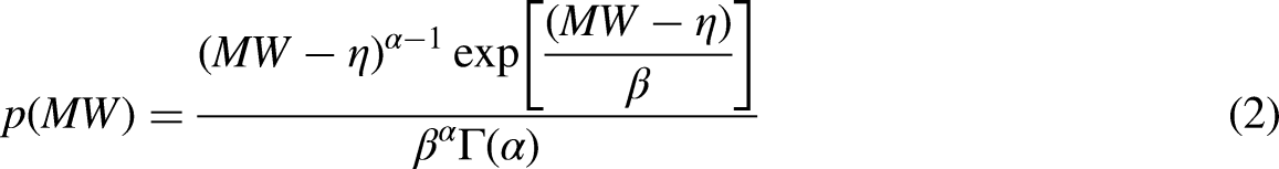

To generate the distribution of C7 to C45,
Range of concentration of components and distribution parameters.
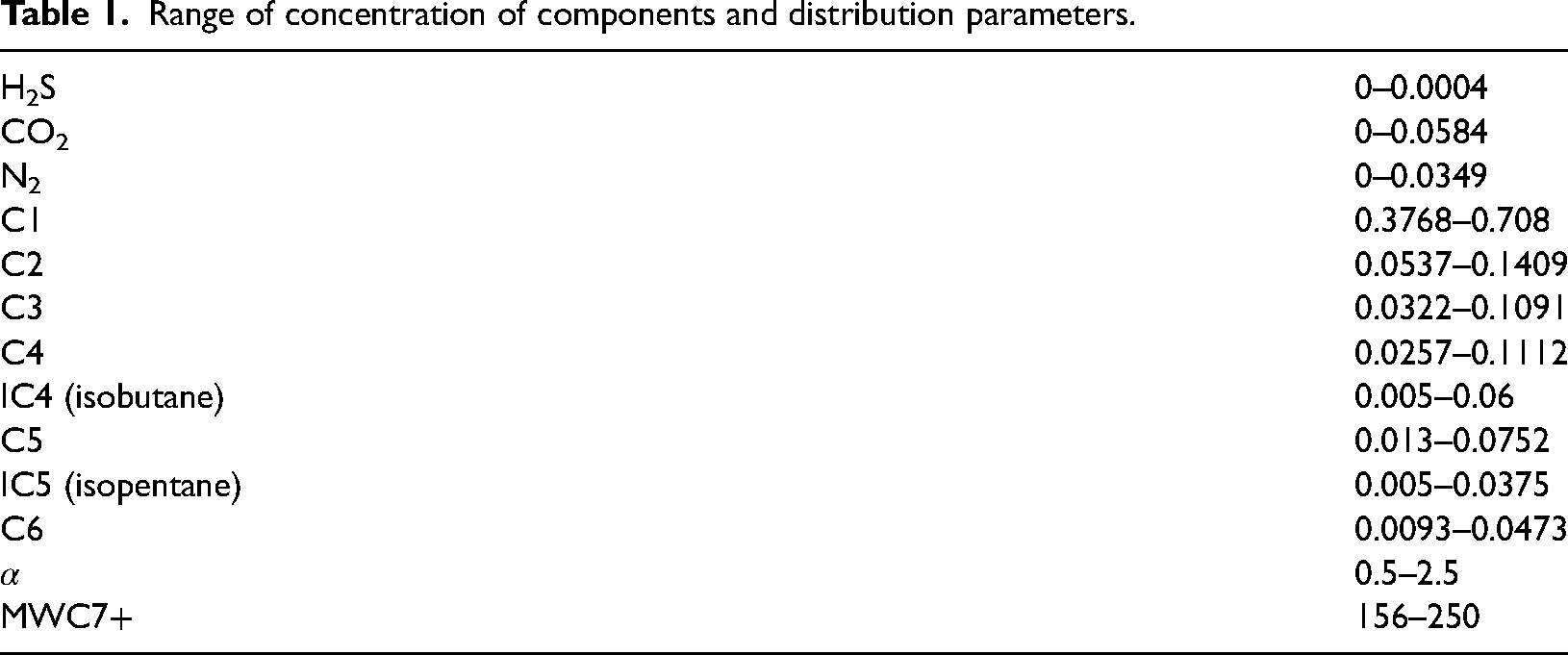
For each set of synthetic volatile oils, a temperature is randomly generated within a given range. Then the bubble-point pressure for the synthetic volatile oil at this temperature is found using a PVT algorithm. The bubble-point pressure is taken to be the initial pressure at the gas–oil contact. If the synthetic oil at this particular temperature is not found in the oil zone at a pressure between 1500 and 10,000 psia, the case is excluded. The composition of the gas in the reservoir at the gas-oil contact is calculated by flashing the oil composition at a pressure 1 psia lower than the bubble-point pressure. Using a radial-cylindrical coordinate system, circular reservoirs are modeled. Implemented is the discretization strategy outlined by Abou-Kassem et al. (2006). Figure 4 demonstrates the structure and design of a sample volatile oil formation. After capillary pressure curves are haphazardly generated for each scenario, the densities of the liquid and vapor phases at the beginning condition are computed and used to infer the length of the transition zone. Then, the well blocks are configured to solely encompass the oil zone. The distribution of contact depths is determined by their respective ranges. Production from the well is done at constant bottom-hole pressure. The starting pressure is multiplied by a chance number between 0.15 and 0.3 to determine the bottomhole pressure. The thickness of the formation multiplied by a chance number between 0.05 and 0.4 determines the distance from the gas–oil contact to the top of the formation. The formation thickness times a chance number between 0.8 and 1 determines the separation between the water–oil contact and the formation top.
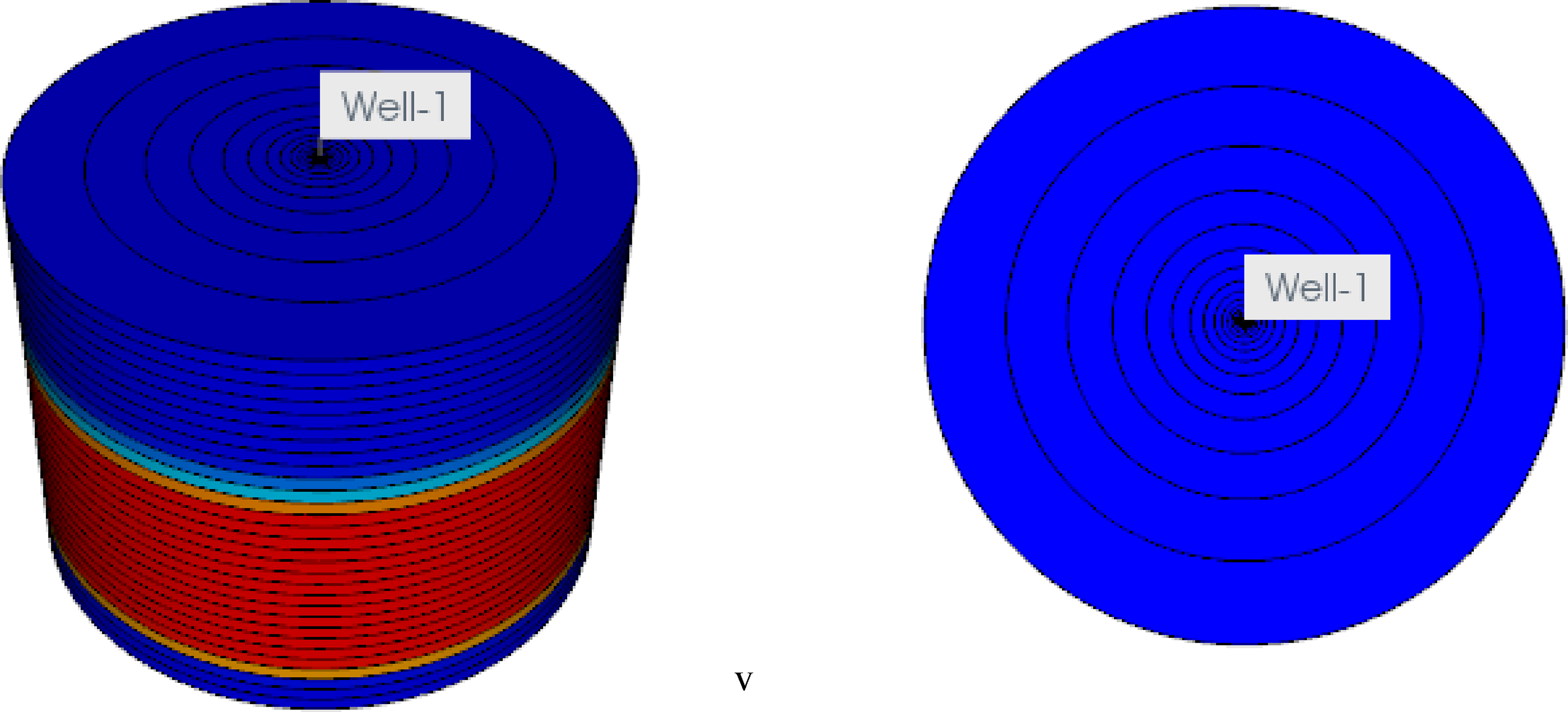
Representation in the forms of a side view and top-down view of a sample volatile oil reservoir. The discretization is demonstrated. The red region in the lower middle part represents the oil zone. The zone above represents the gas zone while that below represents the water zone.
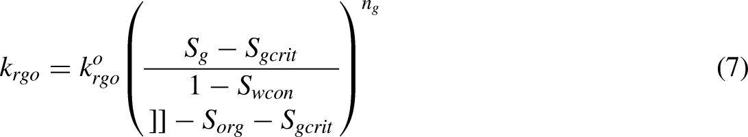
In this work, Stone's Model II and Corey's model are used to model relative permeability. Two power-law formulas serve as representations for capillary pressure. The Corey model's formula is broken down into equations (4) through (7)


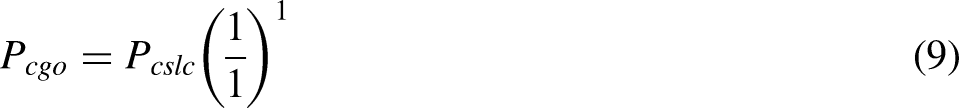
Capillary pressure in the matrix is described by equations (8) and (9) (modified from Gang and Kelkar, 2007).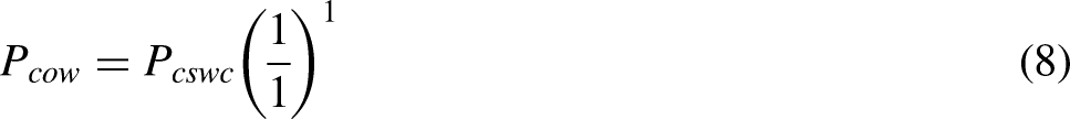
The range of reservoir and fluid properties is given in Table 2.
Range of reservoir and fluid properties.
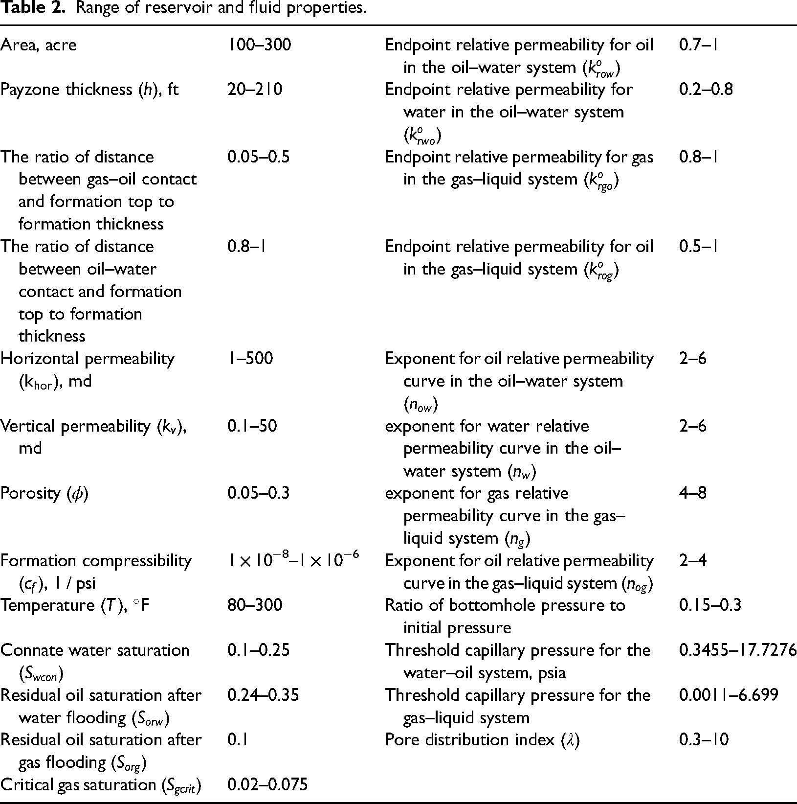
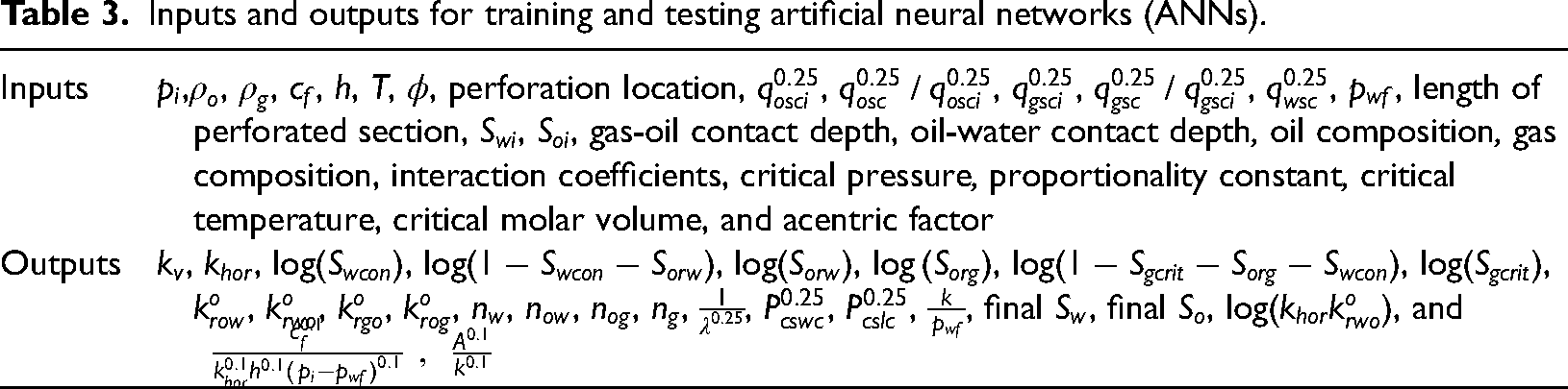
The 50 × 1 × 30 discretization is found to be the best one for modeling volatile oil reserves through sensitivity analysis. The petrophysical property and reservoir fluids configurations as well as the sensitivity analysis results which include the simulation production rates have been demonstrated, plotted, and drawn by Zhang (2017). Researchers who would like to know the details of the comparisons on the simulated production rates (water rates, oil rates, and gas rates) and the identification of the best optimization with the detailed least number of grid blocks and a high accuracy can go check those analyses with delineated details. Circular volatile-oil reservoir models are built and run using this discretization. Table 2 provides the properties’ ranges. In models of circular reservoirs, the ratio of the oil phase to the gas phase at the gas-oil contact is determined and utilized as the model's initial condition. The production data is then extracted from the results files using software. This production data, coupled with reservoir and fluid parameters obtained from well logs and fluid tests, are used as inputs for ANN training. The petrophysical properties employed in the simulation runs are the results used during training. The inputs and outputs are listed in Table 3. Since feedforward ANNs have been successfully used in prior studies on predicting relative permeability, feedforward networks have been employed in this investigation (Guler et al., 2003; Silpngarmlers et al., 2002).
Inputs and outputs for training and testing artificial neural networks (ANNs).
To enable a steady distribution of parameters, a total of 74
Results and discussion
In this study, a three-layer feedforward network with one hidden layer exhibits the best performance. A total of 69 neurons make up hidden layer 1 of the brain (neural network). A symmetric saturating linear transfer function serves as the transfer function for buried layer number 1. Conjugate gradient backpropagation along with Polak–Ribiére updates is used in this training procedure. At the 458th epoch, the training process's lowest performance function is 0.1922. The training ends 500 extra epochs later.
This section compares the expected and actual values of three petrophysical properties: horizontal permeability, vertical permeability, and relative permeability. Additionally supplied are statistics on the predictions made by the ANN. In Figures 5 and 6, permeability comparisons are shown. The predicted horizontal permeability and the observed horizontal permeability were very similar. In terms of horizontal permeability, the average relative error is 13.5%. Although the anticipated and actual vertical permeability differs when compared, the patterns between the two values are quite comparable.
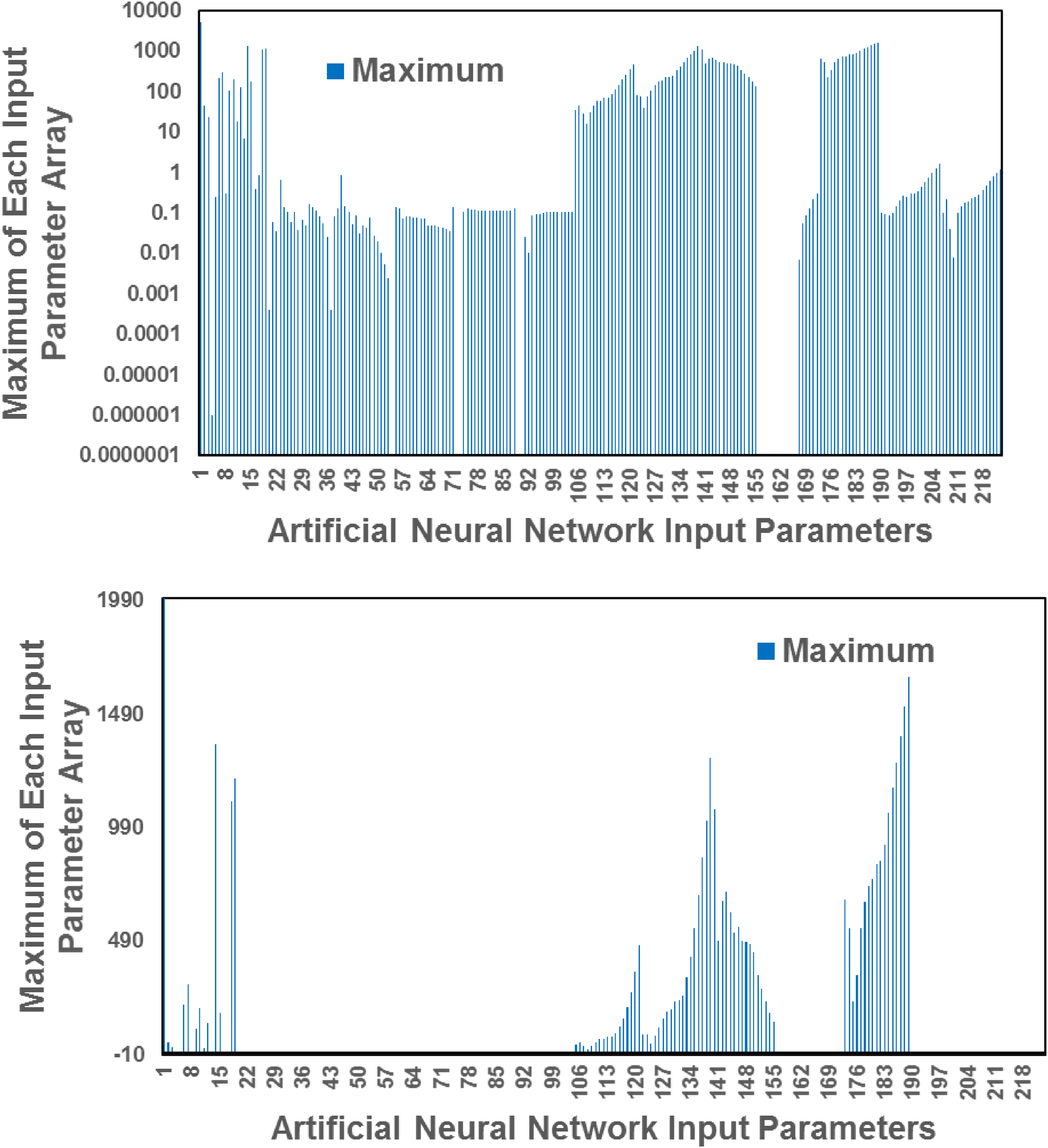
The distribution of a maximum of the parameters used in the training procedure in log scale (upper figure) and in normal scale (lower figure).
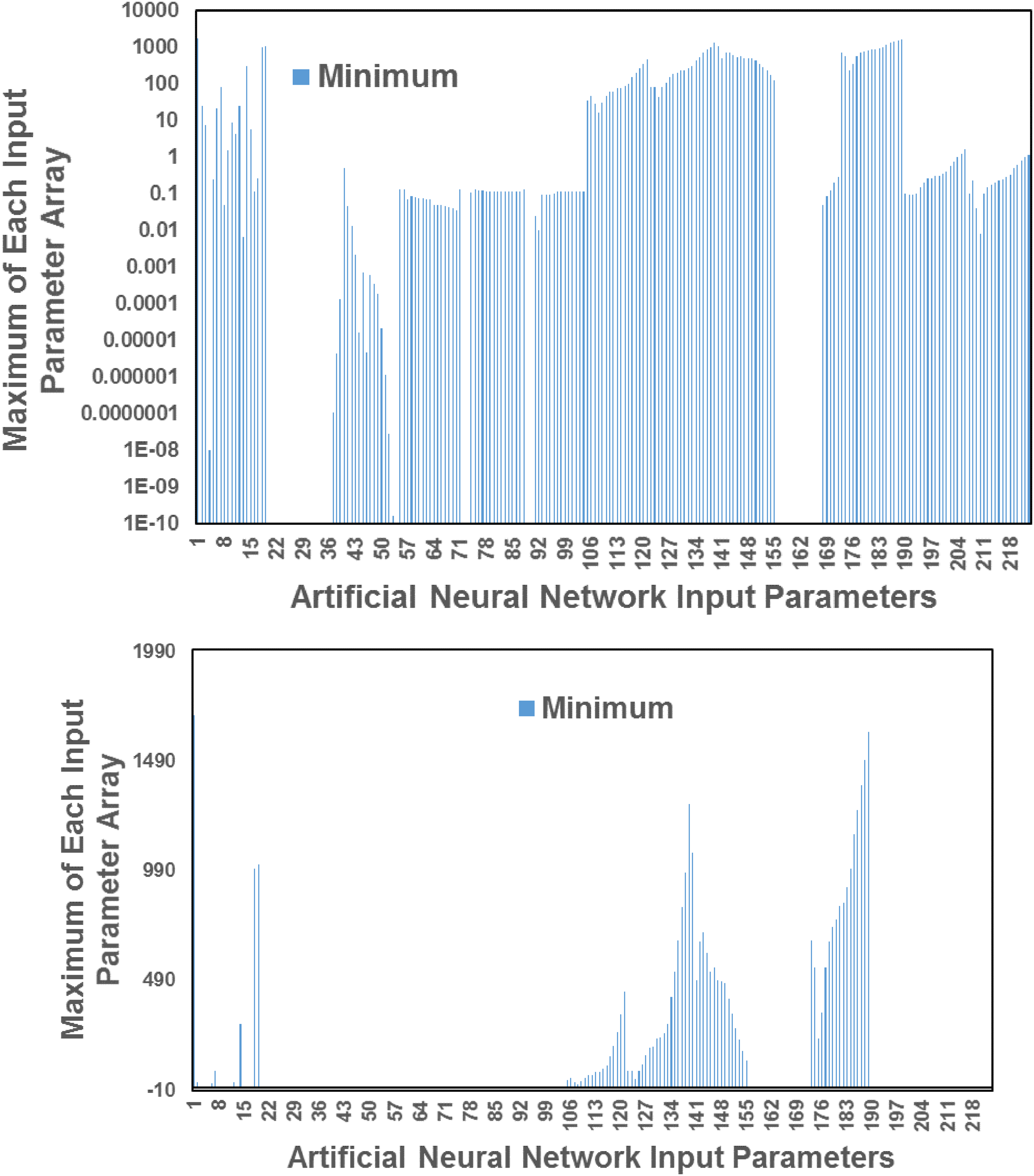
The distribution of minimum of the parameters used in the training procedure in log scale (upper figure) and in normal scale (lower figure).
For the test instances, two-phase relative permeability curves and capillary pressure curves are plotted using both the expected attributes and their actual values. Figures 7 to 11 show the capillary pressure and relative permeability curves for the first five test instances.
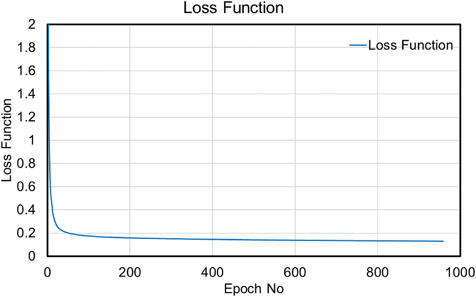
The loss function of the three-phase volatile-oil reservoir petrophysical property prediction artificial neural network training process.
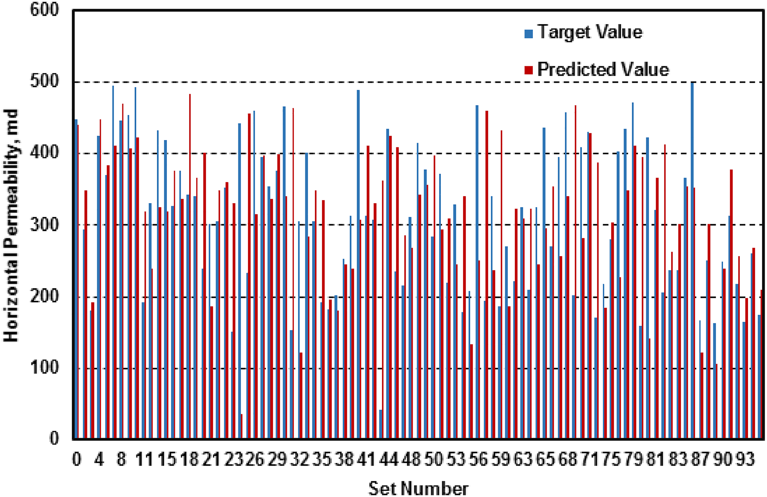
Horizontal permeability of test cases.
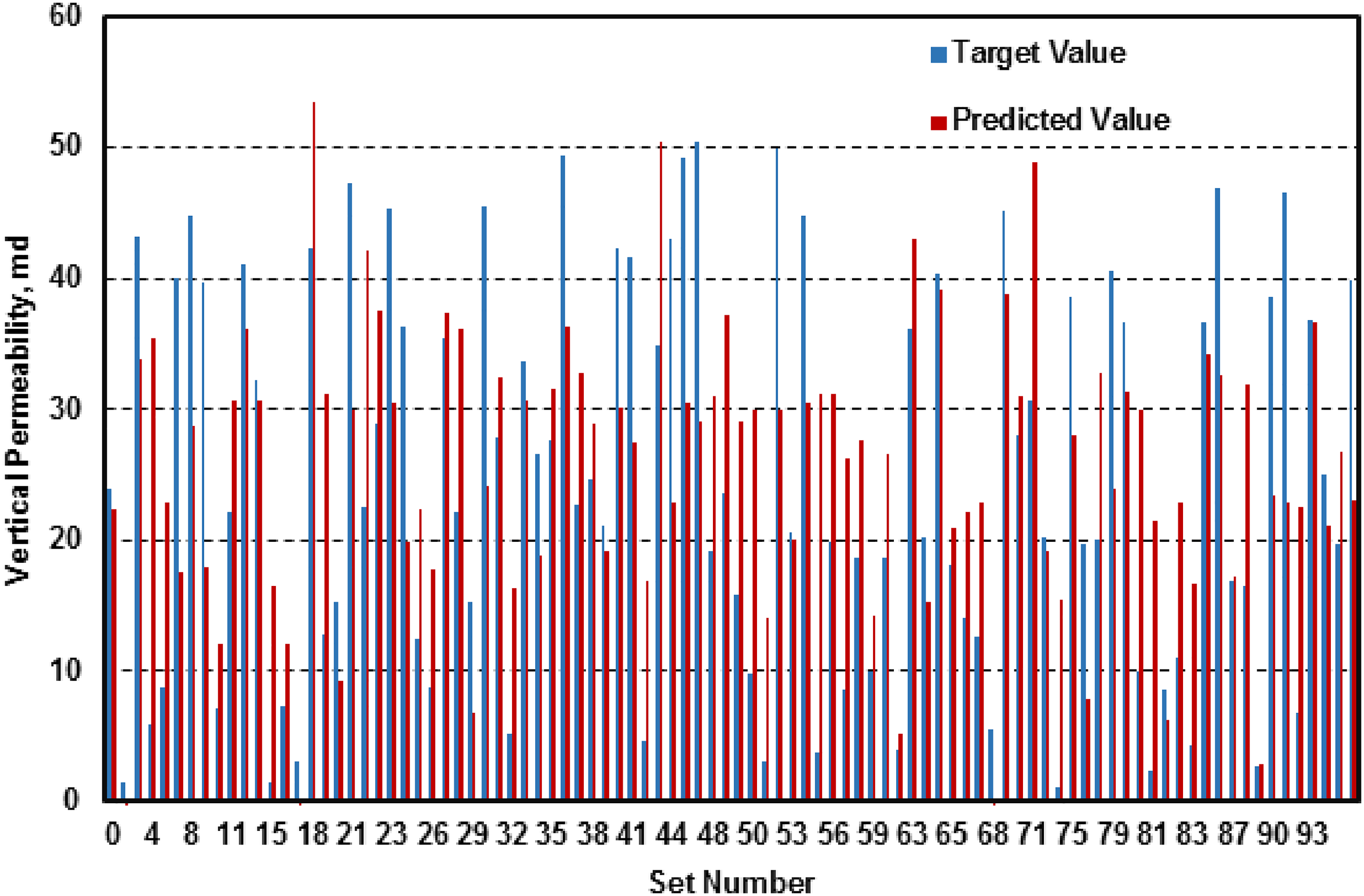
Vertical permeability of test cases.
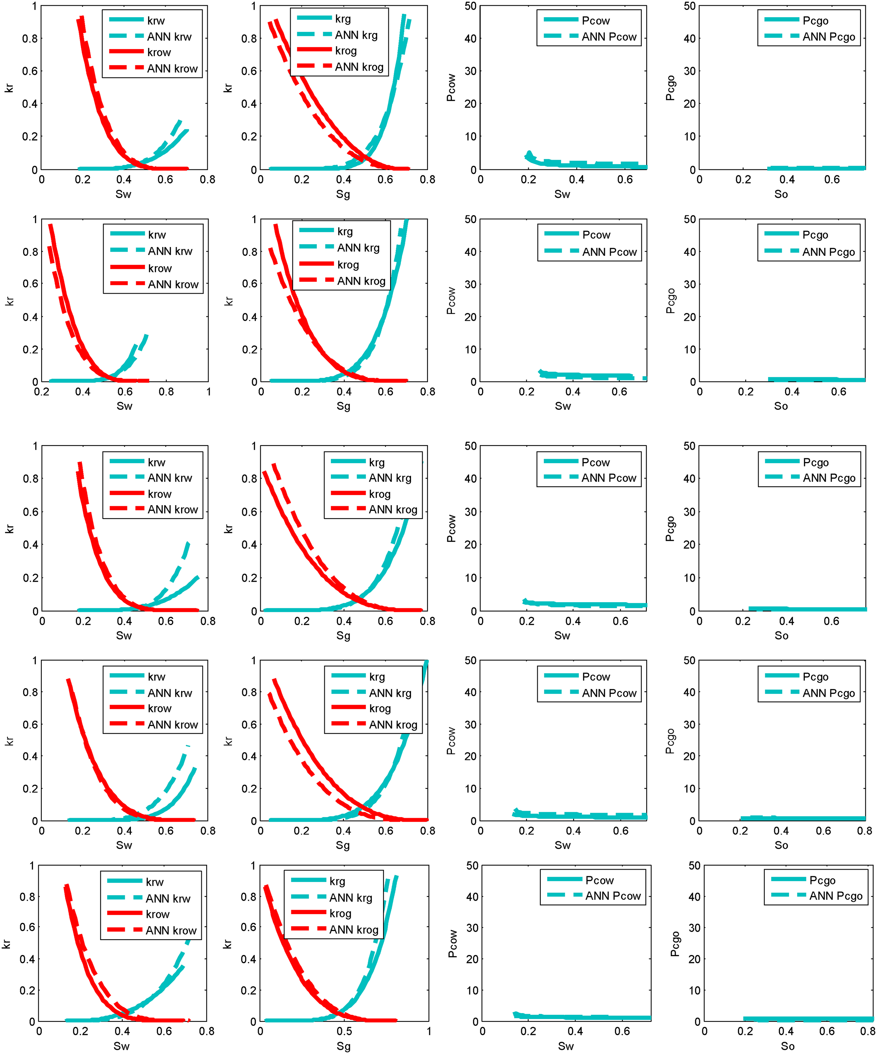
Results of ANN predicted relative permeability and capillary pressure for test cases 1, 2, 3, 4, and 5 in sequence.
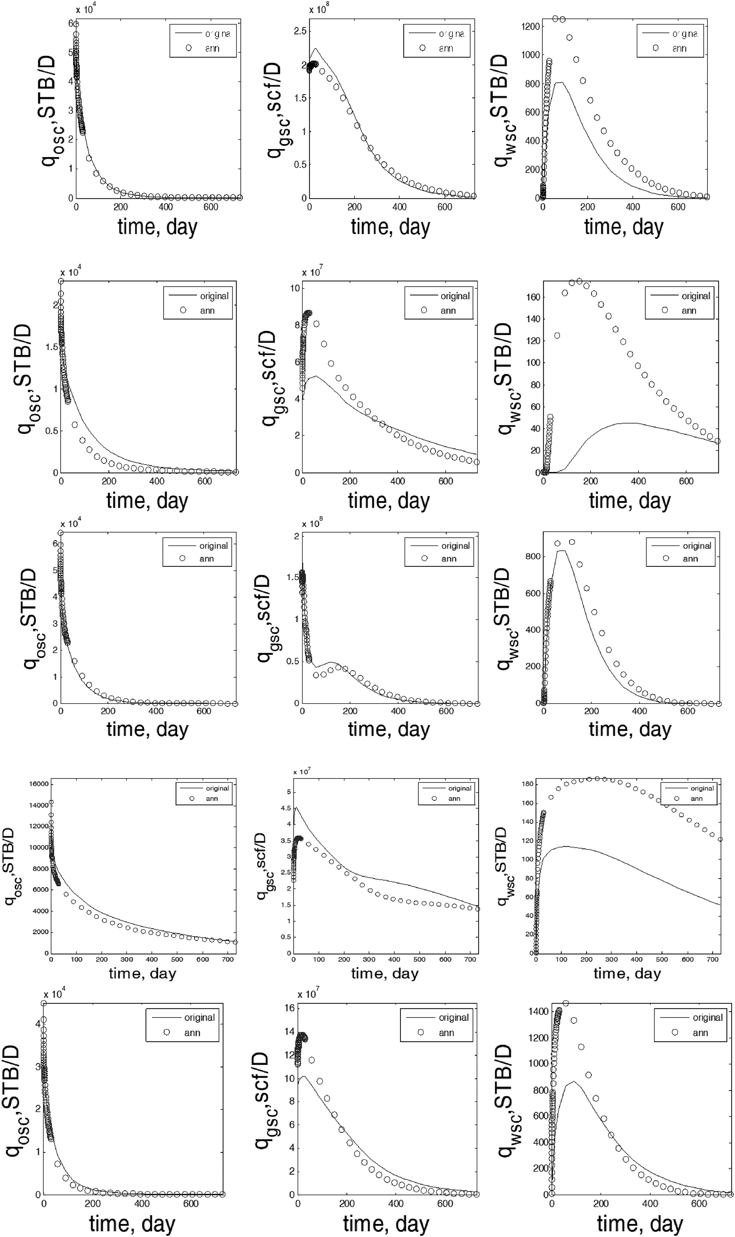
Results of simulated reservoir oil, gas, and water production data using predicted permeability (horizontal and vertical), relative permeability, and capillary pressure compared with those using original reservoir properties for test cases 1, 2, 3, 4, and 5 in sequence.
The comparisons show that the relative permeability curve closely resembles both the capillary pressure curve and the real relative permeability curve. The majority of the test scenarios have similar endpoint relative permeabilities. The relative endpoint saturation error for the water relative permeability curve ranges from −30% to 50%. Between −25% and 30% are the relative errors for the endpoint saturations of the relative permeability curve of oil in the water–oil system. For 87 out of the 95 examples, the relative error for residual gas saturation is between −50% and −50%. For 87 of the 95 cases, the relative permeability curve of water's curvature parameter, or exponent in Corey's model, is between −50% and 50%. Again, the exponent in Corey's model, the curvature parameter for the relative permeability curve of oil in water-oil systems, is between −40% and 50% for 84 of the 95 examples. For 92 out of the 95 examples, the curvature parameter, or exponent, in Corey's model for the relative permeability curve of oil in liquid–gas systems ranges between −30% and 40%. For 88 out of 95 cases, the relative errors of the curvature parameter, or exponent, in Corey's model for the relative permeability curve of gas range from −30% to 40%. Following that, production data is generated using the reservoir models that were built using the projected parameters. To assess the prediction's accuracy, the extracted production data is contrasted with the original production data. Figures 6 to 10 also display a comparison of the output rates for the first five valid test instances. We discovered that, with the exception of four cases, the test cases match in terms of their oil production rates based on comparisons of the production rates for the test cases in these figures. Ten examples reveal an apparent difference in gas rates between the test situations. Half of the cases’ production rates indicate a perfect match between water production rates, while the other half of the cases indicate mismatches.
In some instances, incorrectly anticipated horizontal permeability is the cause of discrepancies between oil production rates and gas production rates. In other instances, the discrepancy between the estimated gas and oil production rates from the updated reservoir models and those from the initial simulations is primarily attributable to incorrect forecasts of the relative permeability curves. The differences in the other circumstances are caused by the combined effects of relative permeability, vertical permeability, and horizontal permeability. An incorrect water relative permeability curve could lead to an imbalance in water production rates. The disparity could potentially be due to incorrect vertical permeability predictions. The inaccurate forecast of horizontal permeability also has an impact on the quality of the production match.
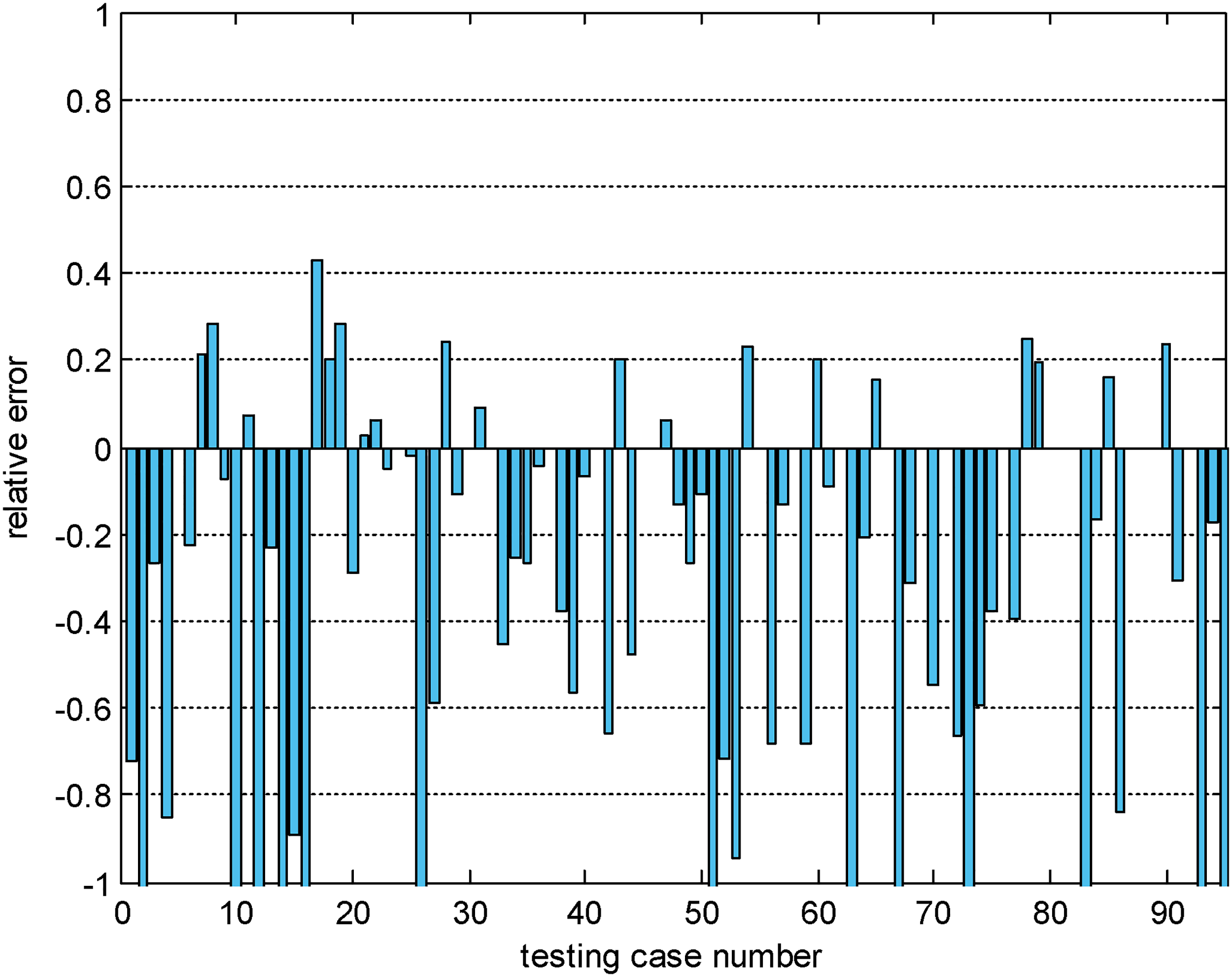
Figures 9 to 11 show the bar plots showing the cumulative relative error in production for the three phases. The relative errors of the non-convergent situations were set to zero. Figures 12 to 14 show the distribution of relative error in cumulative production. The histograms’ horizontal axis ranges must fall between −1 and 1.
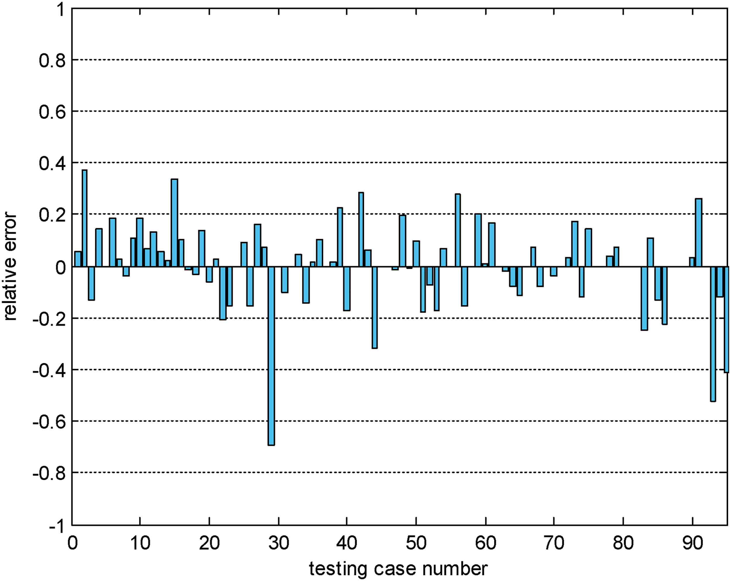
Relative error of cumulative oil production of test cases.
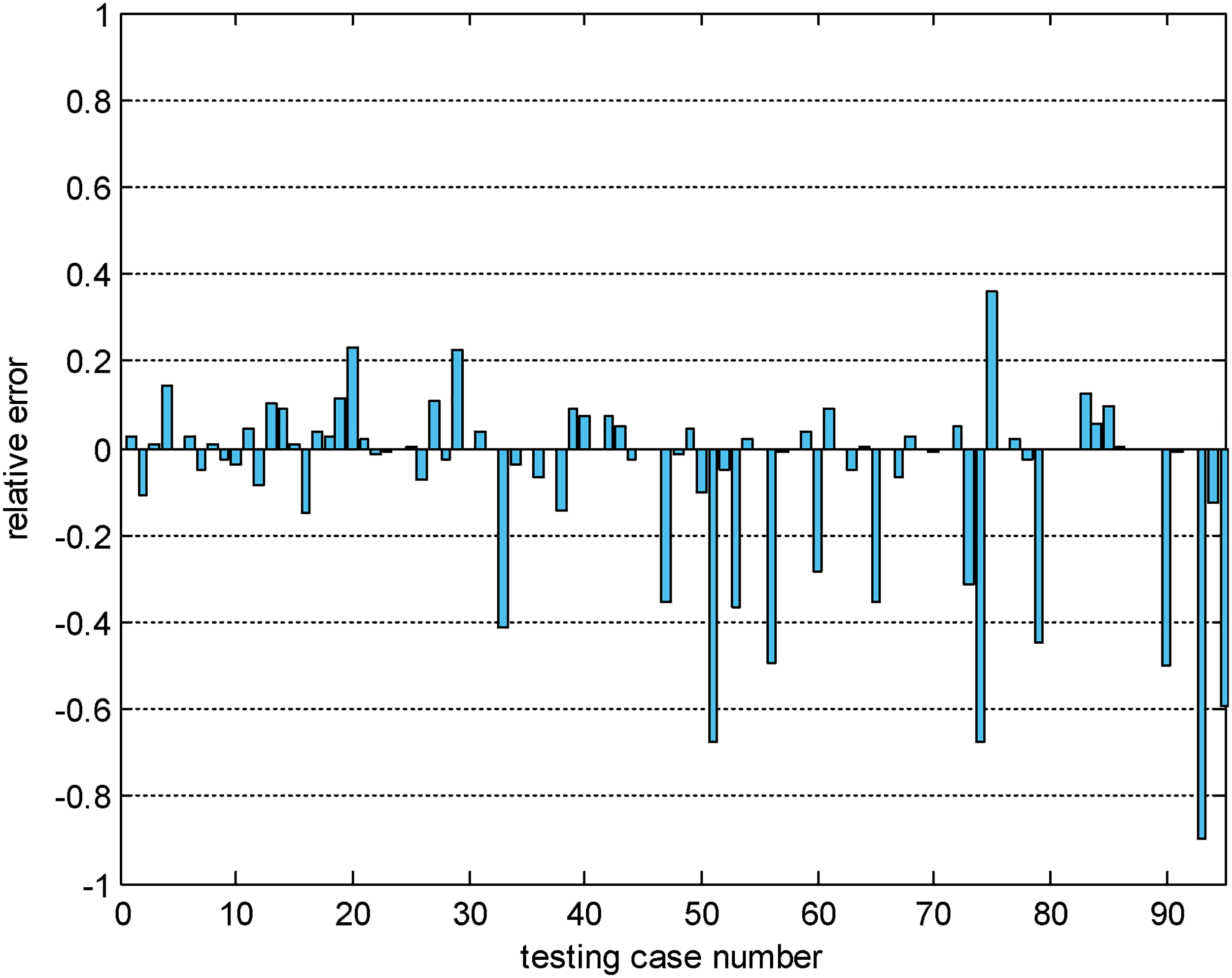
Relative error of cumulative gas production of test cases.
Relative error of cumulative water production of test cases.
In the completed 74 test cases’ simulation running results, 61 reveal relative errors in cumulative oil output between −20% and 20%, excluding the simulation runs that fail to converge. Similar to this, 58 out of 74 test instances show relative inaccuracies in the cumulative output of gas between −20% and 20%. The results of 66 of 74 testing instances point to relative errors in cumulative gas output between −40% and 40%. Moreover, 44 test instances reveal relative errors in cumulative water production between −40% and 40%, while 23 test cases show relative errors in cumulative water production between −20% and 20%. The results of the production profile comparisons allow us to draw the conclusion that the ANN tool is able to forecast petrophysical parameters with a great degree of accuracy. For the majority of test cases, the tool's forecasting ability accurately describes oil and gas production rates. Despite the fact that the water production rates of simulations with predicted parameters are less precise than the oil and gas production rates, the ANN tool is still able to produce correct findings for half of the scenarios.
It should be noted that other than the mean squared error with weighted mean squared weight, mean squared error (MSE) and mean absolute error (MAE) performance functions were also implemented following the training process in order to validate against the training results. The predicted permeability, both horizontal and vertical, from the trained ANN compared against the original values are shown in Figures 15 to 18. The MAE of the predicted horizontal permeability from the network trained using MSE plus mean squared weight is 96.78 md while the MAE of the vertical permeability from the same neural network is 28.2 md. The MAE of the prediction on horizontal permeability from the neural network trained using MSE as the measure for training performance gives an MAE of 66.35 md. The error of predicted vertical permeability by the network generated using the training process using MSE is 10.33 md. Using MAE as the error function of the network training process gives a neural network predicting horizontal permeability with a 55 md MAE and vertical permeability with a 10.46 md MAE. We could observe that the prediction errors with MAE and MSE are lower than those from the network trained with MSE added with a weighted sum of squared weights. This may be due to the reason that weight is not strongly correlated to the accuracy of the prediction results of the petrophysical properties. The error of the horizontal permeability prediction from the ANN trained using MSE as the error function is slightly larger than that obtained from that trained using MAE as the error function. This may be explained using the statement that MAE could more evenly represent the error distributed within the horizontal permeability range. All predictions using the three different kinds of error functions fall into a range that is considered good estimations as the predicted values and the real values are close.
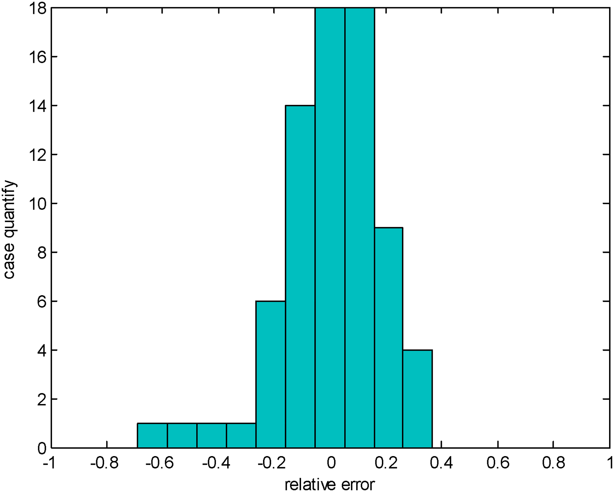
Distribution of relative error of cumulative oil production of test cases.
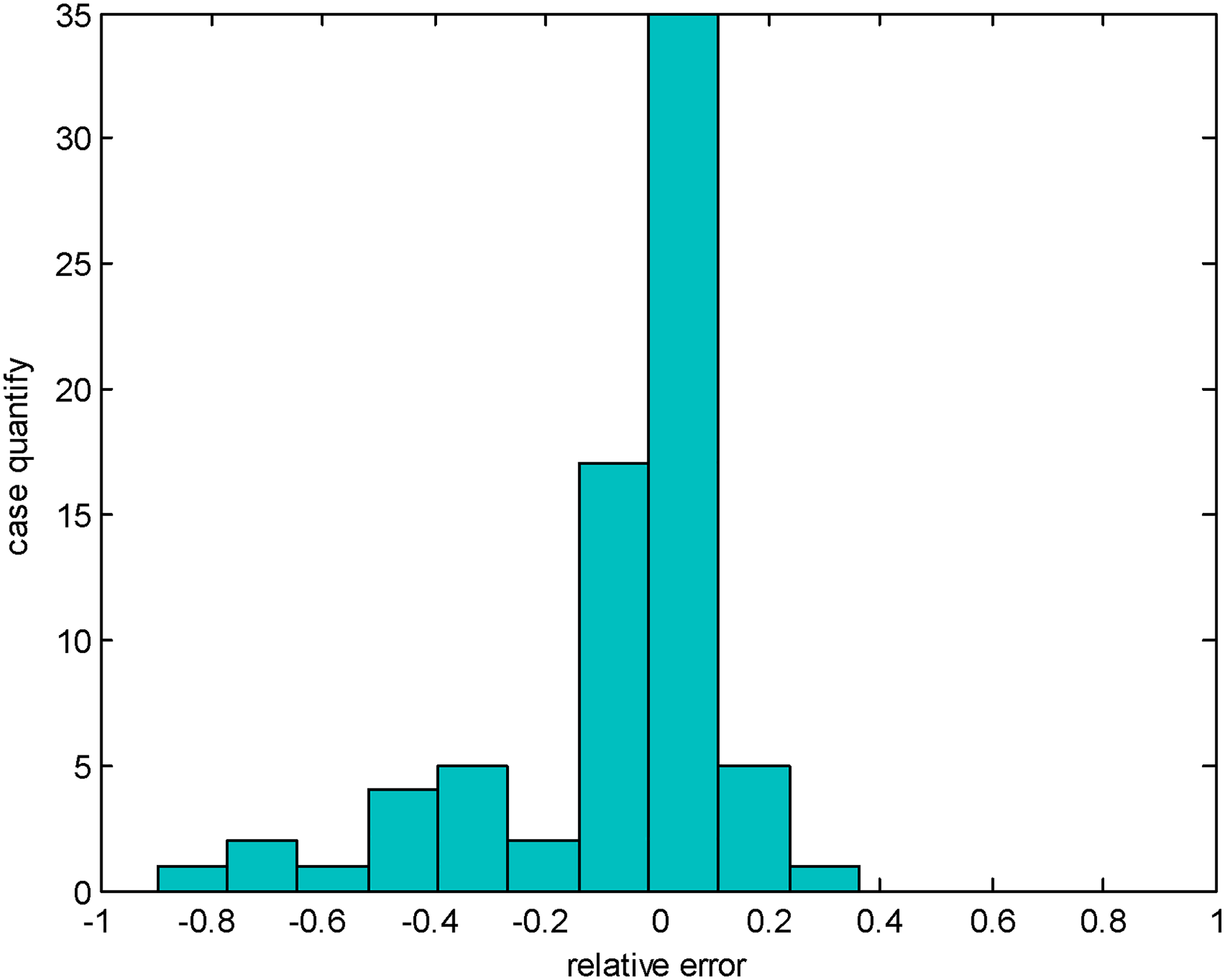
Distribution of relative error of cumulative gas production of test cases.
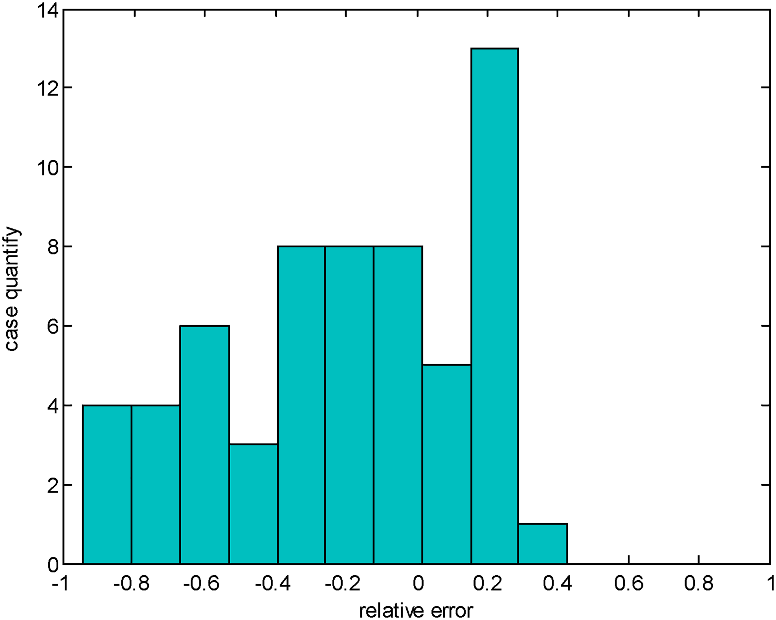
Distribution of relative error of cumulative water production of test cases.
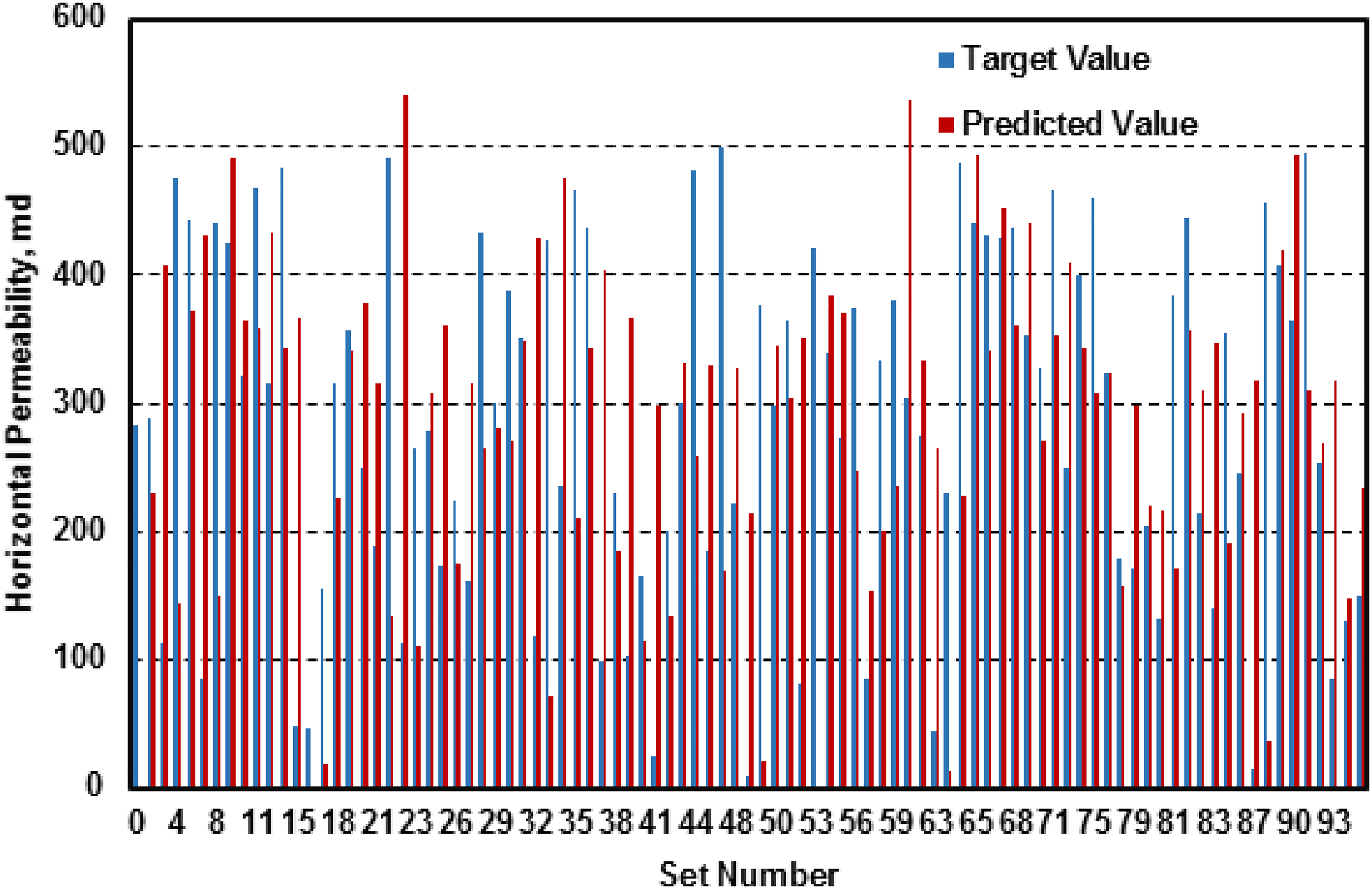
Horizontal permeability of the testing cases from the network generated from the neural network training process using mean square error as the error function.
Finally, we create a graphical user interface that can be used to forecast petrophysical parameters using the created ANN tool, as shown in Figures 19 to 22.
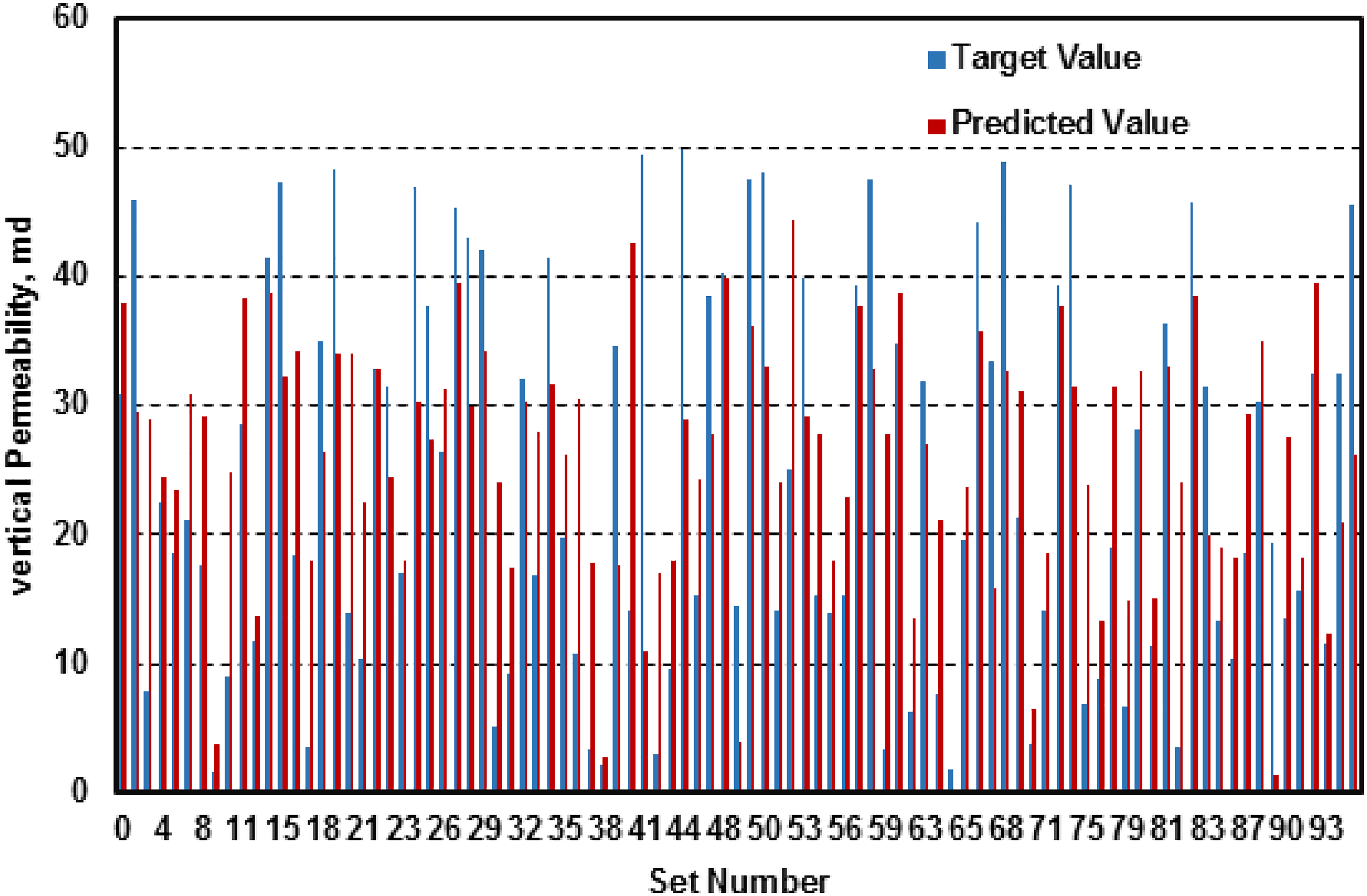
Vertical permeability of the testing cases from the network generated from the neural network training process using mean square error as the error function.

Horizontal permeability of the testing cases from the network generated from the neural network training process using mean absolute error as the error function.
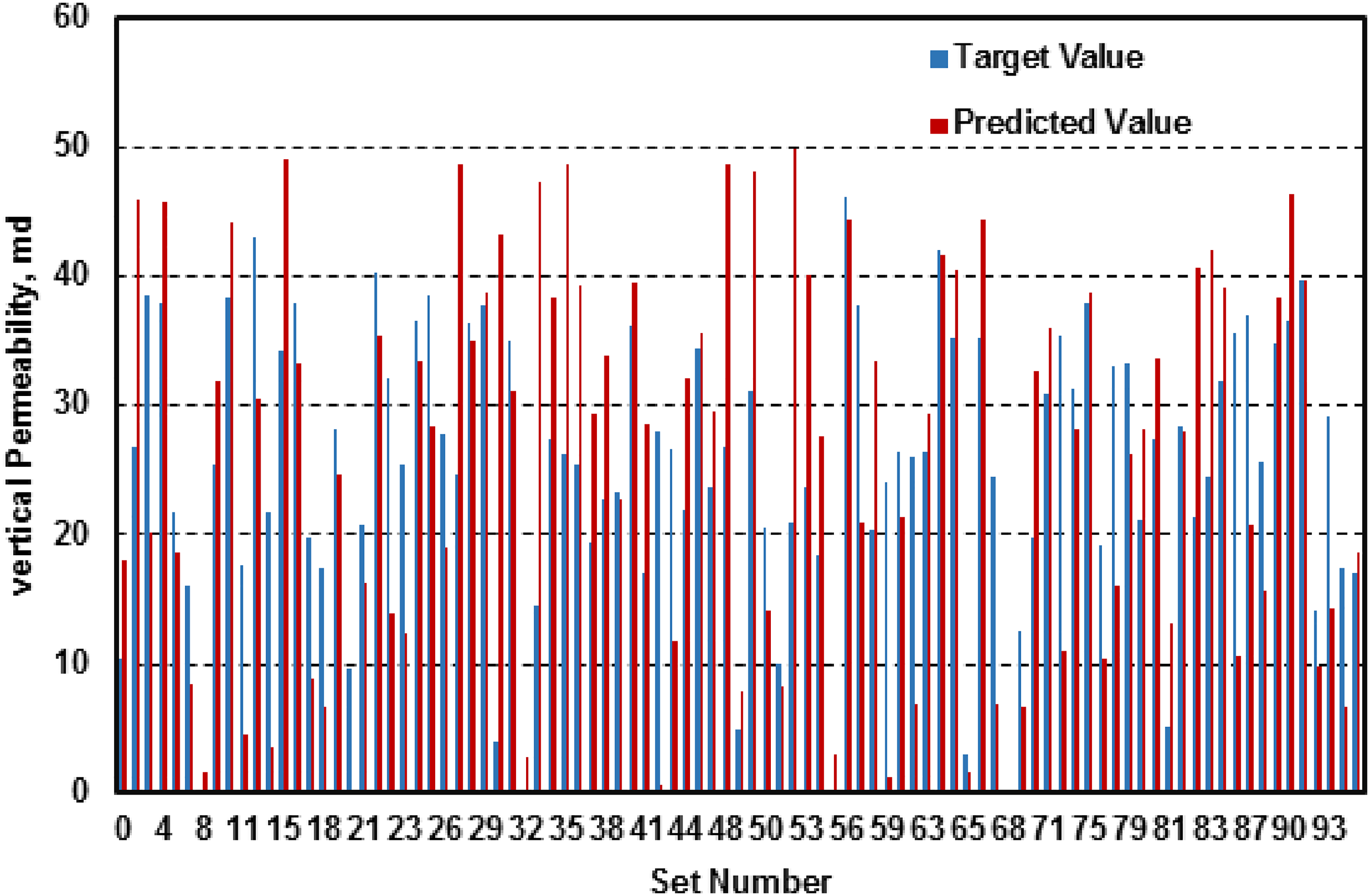
Vertical permeability of the testing cases from the network generated from the neural network training process using mean absolute error as the error function.
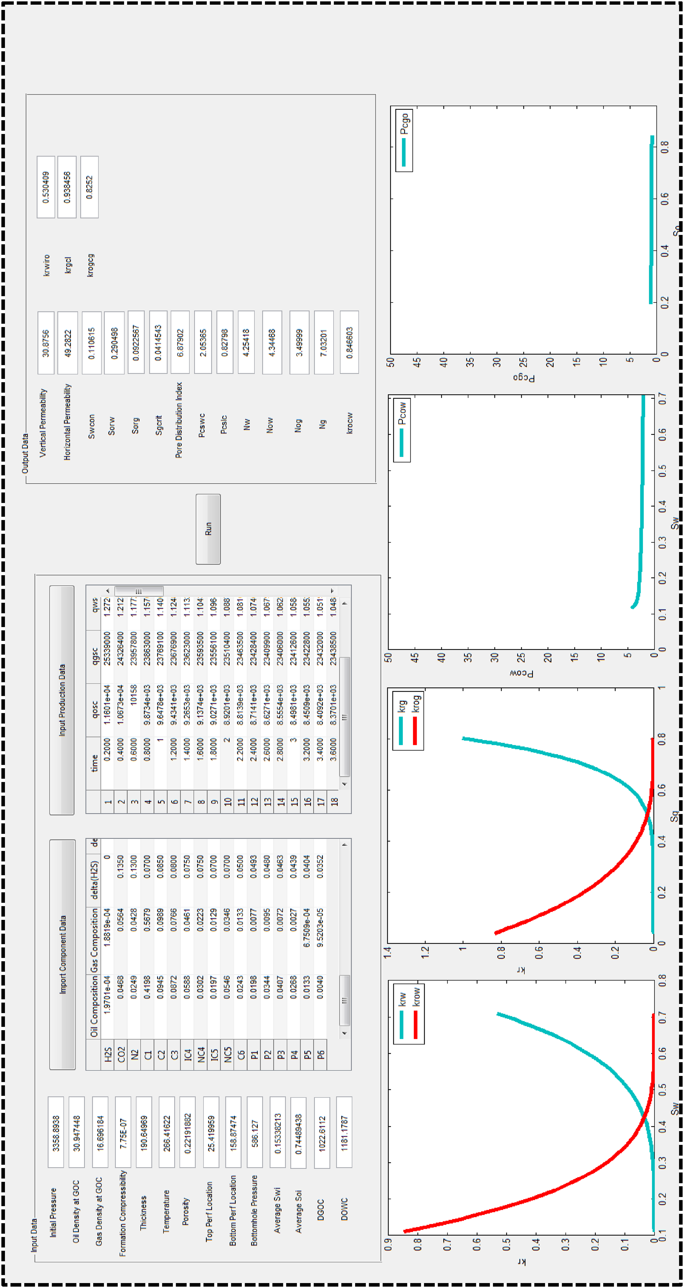
Implementation of graphical user interface (GUI) for circular volatile-oil reservoir with vertical well.
To enforce the developed permeability and relative permeability predicting software in the real field case, a reservoir engineer is supposed to collect readily available field data and reservoir and fluid properties including reservoir initial pressure, oil density, gas density, formation compressibility, reservoir thickness, reservoir temperature, porosity, perforation location, oil production rates, gas production rates, water production rates, bottomhole pressure, length of the perforated section, initial water saturation, initial oil saturation, gas–oil contact depth, oil–water contact depth, oil composition, gas composition, interaction coefficients, critical pressure, proportionality constant, critical temperature, critical molar volume, and acentric factor. Then the reservoir engineer applies the data to the input section of the software and runs it. Then the reservoir engineer will obtain the permeability, relative permeability, and capillary pressure curve estimation, which the reservoir engineer could use in reservoir simulation studies or rate transient analysis to estimate reserve and forecasting future production. More than this, the researchers, when implementing real field case data in their analytical solutions and reservoir numerical simulations, could use the tool to predict the permeability, relative permeability, and capillary pressure and use the predicted values as initial guess in their analytical solutions and numerical simulation runs data inputs.
It should be realized that this ANN tool for predicting three-phase relative permeability relationship and horizontal and vertical permeability and capillary curves is limited to the application in volatile oil reservoir scenarios without the open outer boundary which ideally should be closed. Also, the fluid properties, permeability, porosity, and thickness should strictly fall within the developer-assigned property range of those values in order for this developed tool to be strictly applicable to the scenario in the case of the tool's application.
Conclusions
In this study, we created an ANN-based expert system to assess the capillary pressure curves and three-phase relative permeability, as well as other petrophysical parameters. Our newly created ANN technology is concentrated on compositional volatile oil reservoirs. In blind tests, the developed tool has been shown to correctly forecast the majority of three-phase relative permeability relationships, capillary-pressure curves, and other petrophysical parameters. The input data can be easily obtained from drilling, completion, well logging, and PVT tests.
A huge number of reservoir models covering a broad range of reservoir and fluid parameters are produced in order to generate the ANNs. The reservoir attributes and production data that were taken from the results were converted into a training data format and applied to the training. A large amount of ANNs were trained and the best-performing network was selected. To evaluate the network's performance, the ANNs were put to the test with blind cases. The best-performing ANN is then selected for use.
After conducting the simulations of the updated models, we substituted the original petrophysical properties with the predicted ones and obtained production data to examine the accuracy of the predicted petrophysical properties for blind test cases. We see a reasonable match between the production profile from the revised model and the outcomes from the previous original model for the vast majority of the testing situations. As a result, we are confident that the trained ANNs can make precise predictions in a range of scenarios. However, there are also instances where expert systems are unable to anticipate an accurate outcome, suggesting that we should use caution while using the ANN.
The ANN predicts residual saturation, critical saturation, and connate water saturation in addition to three-phase relative permeability, capillary pressure, and permeability. The tool offers efficient help with reservoir modeling and history matching. The tool can be used to assess the petrophysical characteristics of the reservoir as the input into analytical/numerical models when history-matching work runs into local minimums.
Additionally, this instrument is a useful source of petrophysical data for the petrophysical characteristics of uncored wells.
Footnotes
Acknowledgements
The authors would like to thank John Yilin Wang, Ming Xiao, and Hamid Emami-Meybodi for their valuable comments throughout the study. The authors would also like to thank Bob Brugman from CMG and Gregory King for their precious help in reservoir simulations.
Declaration of conflicting interests
The author(s) declared no potential conflicts of interest with respect to the research, authorship, and/or publication of this article.
Funding
The author(s) disclosed receipt of the following financial support for the research, authorship, and/or publication of this article: This work was supported by The Pennsylvania State University (grant number N/A).