A Machine Learning Workflow to Support the Identification of Subsurface Resource Analogs

Abstract

Identifying subsurface resource analogs from mature subsurface datasets is vital for developing new prospects due to often initial limited or absent information. Traditional methods for selecting these analogs, executed by domain experts, face challenges due to subsurface dataset's high complexity, noise, and dimensionality. This article aims to simplify this process by introducing an objective geostatistics-based machine learning workflow for analog selection.

Our innovative workflow offers a systematic and unbiased solution, incorporating a new dissimilarity metric and scoring metrics, group consistency, and pairwise similarity scores. These elements effectively account for spatial and multivariate data relationships, measuring similarities within and between groups in reduced dimensional spaces. Our workflow begins with multidimensional scaling from inferential machine learning, utilizing our dissimilarity metric to obtain data representations in a reduced dimensional space. Following this, density-based spatial clustering of applications with noise identifies analog clusters and spatial analogs in the reduced space. Then, our scoring metrics assist in quantifying and identifying analogous data samples, while providing useful diagnostics for resource exploration.

We demonstrate the efficacy of this workflow with wells from the Duvernay Formation and a test scenario incorporating various well types common in unconventional reservoirs, including infill, outlier, sparse, and centered wells. Through this application, we successfully identified and grouped analog clusters of test well samples based on geological properties and cumulative gas production, showcasing the potential of our proposed workflow for practical use in the field.

Introduction

Analog selection is one of the most arduous tasks related to subsurface resource modeling, essential for groundwater, mineral mining, and hydrocarbon extraction. This is because subsurface datasets are generally highly dimensional (include many features), sampled from complicated heterogeneous and nonstationary phenomenon, and often with biased and extremely sparse sample coverage, combined with the imposition of physics, engineering, and geological constraints (Pyrcz and Deutsch, 2014; Tan et al., 2014). Analogs are comparable scale-dependent systems with similar characteristics and properties to support less well-constrained study intervals. Analog datasets for subsurface resource models include well cores and logs, drill holes cores, drill cuttings, seismic and other forms of remotes sensing and production such as fluid flow rates and run-of-mine mineral grades (Howell et al., 2014; Gravey et al., 2019; Bouayad et al., 2020; Prior et al., 2021). The similarity between these systems is predicated on predefined geological and engineering exploitation attributes. Information types extracted from subsurface resource analogs are the prediction of reservoir univariate, multivariance, and spatial distributions, for example, petrophysical features (e.g., permeability, porosity, and fluid saturations), geological features (depositional style, alteration style, sediment provenance, and structural framework). Thus, subsurface resource analog selection, the choice of what analog to use across various scales and study intervals, is important to constrain subsurface resource model input univariate, multivariate, and spatial distributions. Although there are numerous uses of analogs in the subsurface, a couple prominent ones are the use of production data from existing wells as analogs for future wells to generate a type-curve for well hydrocarbon production over time during prospect evaluation and field estimation (Sidle and Lee, 2010; Rodríguez et al., 2014; Sun and Pollitt, 2022), and mining mineral deposit analogs help identify new prospecting targets (Prior et al., 2021). Accurate subsurface resource analog selection is crucial because an inappropriate analog can lead to erroneous information to populate models and become a source of imprecise and inaccurate subsurface uncertainty model predictions.

Decision making for subsurface resource development is supported by subsurface models constructed by an interdisciplinary team of engineers, geologists, and geophysicists that analyze and integrate all available data types. Poor development decisions result in, for example, drilled oil, gas, and water dry holes, the need for additional wells, and waste rock being sent to the mill. Subsurface resource modeling is characterized by features with multiple nonstationary populations that account for the subsurface system's spatial settings. That is, a multivariate, spatiotemporal model based on high-dimensional spatial data. Subsurface datasets are specific examples of big data, given their characterization by data volume, feature variety, sampling velocity, and data veracity (Mohammadpoor and Torabi, 2020). Subsurface data types are from various sources, with their own coverage and scale, and are typically sparsely sampled, uncertain, and incomplete. Usually, when we have a dataset with one or two predictor features (model inputs) and response features (model outputs) to perform inferential analysis that supports predictive modeling, the conventional approach is to apply multivariate analyses or modeling to achieve this objective.

We propose an innovative geostatistics and machine learning-based analog identification workflow that integrates the subsurface dataset's multidimensional predictor feature and spatial location information. The proposed workflow computes the input dissimilarity matrix using a novel combined spatially modified Euclidean and Mahalanobis distance measure to obtain a space of lower dimensionality (LD) via metric multidimensional scaling (MDS) to mitigate the curse of dimensionality while improving interpretability while adaptively integrating spatial and multivariate information. To address the issue of multiple nonstationary populations and repeatability, kriging of the features and clustering analysis is performed using DBSCAN to identify subgroups in the LD space to maximize information extraction. Lastly, for inferential statistical analysis in the LD space, we introduce new metrics, group consistency score (GCS), and pairwise similarity scores (PSS) for ranking and interpretation purposes. Our proposed workflow addresses the subsurface's multivariate spatial problem of analog selection by providing a robust and generalizable framework for spatial analog identification to support inferential analyses and decision making in highly dimensional datasets.

The background section comprehensively accounts for previous work and linkages on high-dimensional data, data science, and geostatistical concepts. The methodology section details the computation of spatial, multivariate dissimilarity metric with spatial weights for MDS dimensionality reduction, cluster analysis in the reduced dimensionality space via DBSCAN, and mapping in low-dimensional space with ordinary kriging. Furthermore, the section delineates the identification of subsurface resource analogs coupled with GCS and PSS rankings. The results and discussion section describes the oil and gas datasets in high- and low-dimensional spaces, limitations, and the considerations of our proposed workflow. Lastly, we explore the accuracy and validity of the proposed subsurface analog resource workflow concerning well types commonly found and drilled in unconventional reservoirs.

Background

Challenges of high-dimensional data

As the number of predictor features increases, there are new challenges related to working in high-dimensional space, known as the curse of dimensionality. The curse of dimensionality makes it difficult to train and build machine learning models and to find analogs in the subsurface due to challenged data visualization, distance concentration, sparse data sampling and coverage, and feature multicollinearity. Visualization refers to performing an ocular inspection of data and models, such as checking for data outliers, distribution modes, and local model prediction bias. Visualization beyond three dimensions requires significant projection and is quite limited. Distance concentration is the loss in sensitivity in distance measures, often stated as a distance-based loss. This is mathematically described as the distance variances between randomly selected data pairs. It follows that the difference between the maximum and minimum data pair distances goes to $0.0$ as the dimensionality, $d$ , increases (equation (1)). This affects data analytics and machine learning methods, which rely on some notion of distance or dissimilarity as the range of pairwise distances between random points collapses (Aggarwal et al., 2001; Kabán, 2012; Giannella, 2021).

$$if\lim {}_{d\to \mathrm{\infty }}\mathrm{var}\left({\displaystyle \frac{{\Vert X_d\Vert }_k}{\mathbb{E}{\Vert X_d\Vert }_k}}\right)=0,\mathrm{then}{\displaystyle \frac{{D_{\max }}_d^k-{D_{\min }}_d^k}{{D_{\min }}_d^k}{\to }_{p}0,}$$

(1)

$${D_{\min }}_d^k=\min \{{\Vert X_d\Vert }_k\},$$

$${D_{\max }}_d^k=\max \{{\Vert X_d\Vert }_k\}.$$

where k is the value of the norm, $X_d$ the data point from a $d$ -dimensional data distribution with its respective coordinates, while ${D_{\min }}_d^k$ and ${D_{\max }}_d^k$ are the nearest and farthest distance from the origin for all data points, respectively, and $\frac{{D_{\max }}_d^k-{D_{\min }}_d^k}{{D_{\min }}_d^k}$ is the relative contrast ratio, a criterion for distance meaningfulness.

Data sparsity refers to the coverage and sampling limitations in high-dimensional space. Coverage suggests that if the data samples cover $80\text{\%}$ of the range of each feature, then the coverage in two-dimensions and three-dimensions are $64\text{\%}$ and $51\text{\%},$ respectively. Sampling indicates that if $100$ samples are required to inform a univariate histogram, then for a two-dimensional and three-dimensional histogram, $10,000$ and $1,000,000$ samples are required, respectively. In addition, with many features, the likelihood of feature collinearity or multicollinearity increases. Collinearity is the linear association between two predictor features, which explains the same variation in the response feature, whereas multicollinearity is when a feature can be described as a linear combination of more than one other predictor feature.

On account of the curse of dimensionality, analog selection quality may be reduced, resulting in subsurface model inference and prediction error, and suboptimal decision making. Due to its direct monetary implication, representative information extraction from analog workflows is critical during subsurface resource exploitation planning and development. Goode (2002) demonstrated that the lack of a robust and generalizable framework or methodology for accurately obtaining reliable information during inferential analysis costs the petroleum industry approximately $\mathrm{\$}30$ billion annually. For the hydrocarbon resource example, these limitations inevitably introduce error due to poor choice of analogous wells that misinform reservoir feature distributions.

Appropriately using subsurface resource analogs is critical during resource evaluation and reserve estimation (Hodgin and Harrell, 2006; Sidle and Lee, 2010). Despite being an important component, most assessments are made qualitatively, relying exclusively on human expertise, experience, and limited statistical approaches. As a result, analog workflows are subjective, lack reproducibility, and inhibit the establishment of robust best practices. Many attempts have been made over the years to develop quantitative analog methods for either hydrocarbon wells or reservoirs using a variety of reservoir and geological features. For example, close-ology, a scale-dependent strategy used for play evaluation and field development options that employ the qualities and attributes of adjacent wells, reservoirs, or field data as a viable substitute (Cook, 2009; Sun and Wan, 2002). When information is minimal for a drill site, close-ology is often implemented. However, this omits important heterogeneity, spatial continuity, nonstationary trends and regions, domain expertise, and secondary information.

Heterogeneity is the variation quality in petrophysical rock features such as permeability with location. For oil, gas, or water reservoir characterization, heterogeneity specifically applies to variability that affects flow through the porous rock matrix. For subsurface resource modeling, heterogeneity measures are commonly applied to identify analogs. That is, reservoirs with similar heterogeneity metrics should flow similarly (Reese, 1996; Jensen et al., 2000; Fitch et al., 2015). Prevalent examples of such heterogeneity measures in the subsurface are the coefficient of variation of permeability, Dykstra-Parsons, and Lorenz coefficients (Lorenz, 1905; Dykstra and Parsons, 1950; Jensen et al., 2000). However, the heterogeneity estimates from these methods disregard the spatial organization of the feature under consideration and are restricted to univariate analysis only (Jensen et al., 2000; Fitch et al., 2015).

Data science

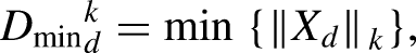
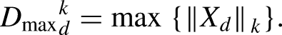
Dromgoole and Speers (1997) pioneered efforts to describe reservoir analogs and complexity for North Sea fields using a field scoring method. This is based on geological complexity and descriptive reservoir features based on high-level interpretations. Bygdevoll (2007) presented a more structured approach, the reservoir complexity index, which assigns analog parameters based on objective parameters and subjective judgment. Data science methods may apply a more general quantitative score based on distance-based dissimilarity, which defines the dissimilarity between pairs of samples through a distance metric. A distance metric exists if it satisfies the conditions of symmetry equation (2), non-negativity equation (3), identification equation (4), definiteness equation (5), and triangle inequality equation (6). For any points (samples in our case), $i_1,i_2,i_3$ , in any dimensional space, a distance-based dissimilarity measure, $d(i_1,i_2)$ , is a distance metric if the criteria are satisfied.

$$d(i_1,i_2)=d(i_2,i_1).$$

(2)

$$d(i_1,i_2)\ge 0.$$

(3)

$$d(i_1,i_2)=0.$$

(4)

$$d(i_1,i_2)=0iff{i}_1=i_2.$$

(5)

$$d(i_1,i_2)\le d(i_1,i_2)+d(i_2,i_3).$$

(6)

With distance metrics, Bhushan and Hopkinson (2002) identified reservoir analogs using the nearest neighbor algorithm to measure the degree of similarity between reservoirs weighted by each reservoir attribute. However, this distance-based approach is disrupted by the previously discussed distance distortion in a higher dimensional space. Rodríguez et al. (2014) address distance distortion in high-dimensional space with principal component analysis (PCA) for dimensionality reduction along with avoidance of multicollinearity between reservoir features (Jollife, 2002; Rodríguez et al., 2014; Jollife and Cadima, 2016). Olukoga and Feng (2022) apply heuristic algorithms, including k-means, k-medians, and hierarchical clustering algorithms, to identify analogous miscible CO₂ flooding projects after applying PCA for dimensionality reduction coupled with a similarity measure using weighted Euclidean distance.

There are various methods for nonlinear dimensionality reduction, such as t-distributed stochastic neighborhood embedding (t-SNE) by van der Maaten and Hinton (2008), uniform manifold approximation and projection (UMAP) by McInnes et al. (2018), and MDS by Torgerson (1952). Although UMAP and t-SNE have been found to outperform MDS as they preserve more of the local structure within the data, both methods do not perform well with sparse and incomplete data (Wang et al., 2021). In addition, Scheidt and Caers (2009) demonstrate that MDS, as a dimensionality reduction method, retains the data's intrinsic structure. Further, Tan et al. (2014) showed that MDS could quantify an uncertainty space.

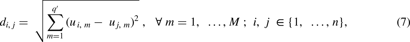
MDS is a nonlinear dimensionality reduction technique that preserves the measure of dissimilarity between pairs of data points by projecting multidimensional data into a lower dimensional space (Kruskal, 1964; Cox and Cox, 2008). Several variations include nonmetric MDS, which uses an iterative approach applicable to ordinal data, and metric MDS, a nonlinear dimensionality reduction method for multivariate datasets that relies on the Euclidean distance function, dissimilarity metrics, or L2 norm. Assuming a distance matrix, $\mathit{D}$ , obtained from a dataset in the multidimensional feature space, ${\mathbb{R}}^d$ , approximates the inter-point distances of a configuration of points yielding projections of reduced dimensionality, $q^{\mathrm{\prime }}$ , where $q^{\mathrm{\prime }}\in \{2,3\}$ . Then, the elements of $\mathit{D},$ denoted by $d_{i,j},$ is calculated from the location vector, $\mathbf{u}$ , in equation (7).

$$d_{i,j}=\sqrt{\sum _{m=1}^{q^{\mathrm{\prime }}}{(u_{i,m}-u_{j,m})}^2},\mathrm{\forall }m=1,\dots ,M;i,j\in \{1,\dots ,n\},$$

(7)

where $u_{i,m},u_{j,m}$ are elements of the location vector of the configuration points, i and $j$ the pair of sample data over the available predictor features, $m$ , belonging to a mathematical set of natural numbers, $M=\{m|m\in \mathbb{N}\}$ in the model from the multidimensional feature space, and n the total number of data pairs.

Cluster analysis is a powerful inferential machine learning method for finding groups in datasets for analog selection. A challenge with common clustering algorithms for cluster analysis, such as k-means clustering, is the predetermination of the number of clusters and other assumptions, such as equal group frequency and convex, spherical groups (Olukoga and Feng, 2022). Density-based spatial clustering of applications with noise (DBSCAN) offers a clustering method without predetermining the number of clusters and the ability to model unequal group frequencies and nonconvex groups (Ester et al., 1996; Schubert et al., 2017). DBSCAN is a hierarchical, bottom-up, agglomerative clustering method that grows clusters over connected patterns using a maximal set of density-connected points. Where sufficient density to form a cluster is defined as having a minimal number of samples within the local neighborhood, which is represented by the model hyperparameters radius, $\epsilon$ , the scale of the local neighborhood, and the minimum number of points, $n_{pts}$ , to meet the density criterion. Samples that fail to meet the criteria are called outliers. DBSCAN clustering is intuitive as the density approach is quite intuitive and performs well for partially overlapping groups.

Geostatistics

Due to subsurface data sparsity, geostatistical concepts are important pre-requisites to understanding subsurface resource analog selection concerning spatial prediction and modeling, that is, spatial continuity modeling with variograms and kriging for spatial estimates with uncertainty. Stationarity is a scale-dependent decision that implies the metric of interest is invariant under translation over a spatial interval. The variogram is a two-point spatial statistic that describes a spatial dataset's degree of spatial variability for any lag vector, direction, and distance, along with an indicator of the maximum distance with spatial dependency, known as the variogram range. Variogram-based modeling is the process of fitting a continuous function to an experimental variogram; therefore, through the integration of spatial structures such as geometric anisotropy, nugget effect, and nonstationary trend, variogram-based modeling quantifies spatial correlation to form predictions to augment sparsely sampled spatial models. Under the assumption of mean, variance, and variogram stationarity, a variogram is defined as

$$2\gamma (\mathbf{h})=\mathbb{E}\{[Z(\mathbf{u}+\mathbf{h})-Z(\mathbf{u})]{}^2\},\mathrm{\forall }\mathbf{u},\mathbf{u}+\mathbf{h}\in \mathrm{SA},$$

(8)

where $2\gamma (\mathbf{h})$ is the variogram often used interchangeably with semivariogram $\gamma (\mathbf{h})$ , $\mathbf{u}$ the coordinate location vector, $\mathbf{h}$ the lag distance vector separating all data pairs, $Z(\mathbf{u})$ and $Z(\mathbf{u}+\mathbf{h})$ for the feature of interest, Z.

The relationship between stationary covariance, $C(\mathbf{h})$ , variogram $\gamma (\mathbf{h})$ , and the variance, known as the sill, ${\sigma }^2$ , shown in Figure 1 and is represented by equation (9) given the ${\sigma }^2$ is standardized to $1.0$ .

$$C(\mathbf{h})={\sigma }^2-\gamma (\mathbf{h}),$$

(9)

Figure 1.

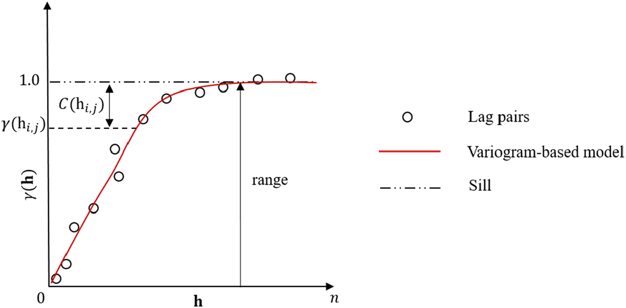
Semivariogram schematic for the normal standardized scores of the feature of interest, $Z^s$ , fit with a variogram-based model, and the sill is $Var\{Z^s\}=1$ .

Kriging is a spatial statistical method for estimating a feature at an unsampled location using available data in the study area and the inferred variogram modeling (Krige, 1951; Matheron, 1962). The kriging methods, for example, simple kriging, ordinary kriging, and universal kriging, are differentiated by their associated decision of stationarity. Ordinary kriging is commonly applied for spatial interpolation and prediction problems in the subsurface due to the flexibility to estimate with a nonstationary mean (Khazaz et al., 2015) and is an unbiased spatial estimator because the data weights add up to one and constrain the estimator while minimizing error variance (Matheron, 1962; Journel and Huijbregts, 1976; Pyrcz and Deutsch, 2014).

Methodology

Our proposed subsurface resource, spatial multivariate analog identification workflow, includes the following steps:

Calculate and model the variogram of the standardized feature of interest, $Z^s$ .

Determine the spatial weights from the standardized response feature.

Compute the dissimilarity matrix input, $\mathit{D}$ , via the proposed dissimilarity metric.

Perform metric MDS on $\mathit{D}$ to obtain the LD space projection output from step (3) in ${\mathbb{R}}^{q^{\mathrm{\prime }}}$ .

Determine the variogram model and kriged estimates for the response in Euclidean space.

Perform ordinary kriging on each feature of interest, Z, in the LD space.

Create a trend map for all predictor features based on the kriging estimates in step (6).

Perform cluster analysis via DBSCAN in the LD space to identify analog clusters.

Identify the centroid of each analog cluster and assign it as a spatial analog in the LD space.

Finalize the workflow and evaluate the proposed ranking and interpretation metrics, GCS and PSS, for data samples in the LD space.

The first step of our proposed workflow for subsurface resource analog identification is to calculate and model the variogram to obtain $\gamma (\mathbf{h})$ . Each feature of interest (i.e., the predictors and response), Z, are transformed separately to a standard normal distribution to obtain the corresponding standardized feature of interest, $Z^s$ , such that $Z^s\sim \mathrm{N}(0,1)$ . This is performed to assist with outlier mitigation, provide improved variogram interpretations, and remove the impact of differences in dispersion (and units) on metric MDS in the proposed workflow. The experimental variograms for $Z^s$ over the lag distance vector, $\mathbf{h}$ , is calculated along the major direction of spatial continuity, ${\theta }_{\mathrm{maj}}$ , with its major and minor ranges denoted as $h_{\mathrm{maj}}$ and $h_{\min }$ , respectively. Then, positive definite nested variogram structures are combined to fit a variogram-based model to these experiential variograms in the major direction of spatial continuity and its orthogonal direction.

Next, the novel dissimilarity metric is calculated that applies the variogram to adaptively weight the spatial and multivariate feature contributions into the dissimilarity matrix, $\mathit{D}$ shown in equations (10) and (11) in the spatial and multivariate feature spaces via standardized features. Since each contribution satisfies the distance metric criteria explained in the Introduction section, adding both relative contributions gives a distance-based dissimilarity that is also a distance metric.

$$d_{SM}(i,j)=d_S(i,j)+d_M(i,j),$$

(10)

$$d_{SM}(i,j)=\sqrt{{\gamma }_R({\mathrm{h}}_{i,j})[{(u_{i,X}-u_{j,X})}^2+{(u_{i,Y}-u_{j,Y})}^2]}+\sqrt{C_R({\mathrm{h}}_{i,j}){(z_{i,m}-z_{j,m})}^T{C}_{z_i{z}_j}^{-1}(z_{i,m}-z_{j,m})},$$

(11)

where $d_{SM}(i,j)$ is the proposed spatial multivariate dissimilarity metric, $d_S(i,j)$ and $d_M(i,j)$ the dissimilarity metrics that account for the spatial and multivariate contributions of the data, respectively. $(u_{i,X},u_{i,Y})$ and $(u_{j,X},u_{j,Y})$ represent elements of the location vector, $\mathbf{u}$ , for respective $i,j$ data pairs in Euclidean space, and ${\gamma }_R({\mathrm{h}}_{i,j})$ the standardized semivariogram model value (sill of 1.0) at a given data pair in Euclidean space for the response feature. $C_R({\mathrm{h}}_{i,j})$ is the stationary covariance between any $i,j$ data pair in the Euclidean space for the response feature, which is the complement of the standardized semivariogram model. $(z_{i,m},z_{j,m})$ denotes the predictor features of interest at any $i,j$ data pair, which is used to compute the multivariate distance between any $i,j$ data pair in the multidimensional feature space while $C_{z_i{z}_j}^{-1}$ is the inverted covariance between any $i,j$ data pair over all predictor features, m, belonging to a mathematical set of natural numbers, $M=\{m|m\in \mathbb{N}\}$ in the feature space.

Modifying the work of de Leeuw and Pruzansky (1978) on weighted Euclidean distance, we propose the novel use of the response features’ semivariogram as the weight to account for spatial contributions applicable only to the location vector, $\mathbf{u}$ , in Euclidean space equation (12). These spatial weights are determined using the geostatistical concepts of the experimental variogram and variogram-based modeling.

$$d_S(i,j)=\sqrt{{\gamma }_R({\mathrm{h}}_{i,j})[{(u_{i,X}-u_{j,X})}^2+{(u_{i,Y}-u_{j,Y})}^2]},$$

(12)

where $d_S(i,j)$ is the dissimilarity metric that accounts for the spatial contribution of the data, ${\gamma }_R({\mathrm{h}}_{i,j})$ the semivariogram value at a given respective $i,j$ data pair in Euclidean space for the response feature. $(u_{i,X},u_{i,Y})$ and $(u_{j,X},u_{j,Y})$ represent elements of the location vector, $\mathbf{u}$ , for respective $i,j$ data pairs in Euclidean space. Next, the work of Mahalanobis (1936) is employed as a novel basis to calculate the dissimilarity metric accounting for the data's multivariate contribution, $d_M(i,j)$ . Consequently, we propose a modified weighted Mahalanobis distance metric employed over all m predictors belonging to a mathematical set of natural numbers, $M=\{m|m\in \mathbb{N}\}$ in the feature space for all $i,j$ data pairs equation (13).

$$d_M(i,j)=\sqrt{C_R({\mathrm{h}}_{i,j}){(z_{i,m}-z_{j,m})}^T{C}_{z_i{z}_j}^{-1}(z_{i,m}-z_{j,m})},\mathrm{\forall }m=1,\dots ,M,$$

(13)

$d_M(i,j)$ is the dissimilarity metric that accounts for the multivariate contributions of the data. $C_R({\mathrm{h}}_{i,j})$ is the complement of the semivariogram for the response feature, while $C_{z_i{z}_j}^{-1}$ is the inverted covariance between any $i,j$ data pair over all predictor features, m, belonging to a mathematical set of natural numbers, $M=\{m|m\in \mathbb{N}\}$ in the feature space. $(z_{i,m},z_{j,m})$ denotes the predictor features of interest at any $i,j$ data pair, which is used to compute the multivariate distance between any $i,j$ data pair in the multidimensional feature space.

Equation (11) shows that the proposed spatial multivariate dissimilarity metric has two end-member cases that result in scenarios where either the spatial dissimilarity metric or multivariate dissimilarity metric suffices for the dissimilarity matrix, $\mathit{D}$ , estimation. The first case occurs when data samples are closely collocated in the Euclidean space, that is, at $C_R(h_{i,j})=1$ . This indicates that only spatial contributions exist, and a fully spatial dissimilarity metric shown in equation (12) is required for $\mathit{D}$ computation. Alternatively, when the variogram range is exceeded, that is, at $C_R(h_{i,j})=0$ , the sole contribution of the dissimilarity metric is from its multivariate contribution, and equation (13) is used for $\mathit{D}$ calculations. Metric MDS is computed using $\mathit{D}$ as input and the location vector in the LD space, ${\mathbf{u}}^{\mathrm{\prime }}$ , within the projection of reduced dimensionality, $q^{\mathrm{\prime }}$ , is obtained.

Next, ordinary kriging is performed on each Z, that is, all predictors and the response features in the LD space to obtain their respective kriged estimates, $Z_{OK}^{*}({\mathbf{u}}^{\mathrm{\prime }})$ , to calculate trend maps that identify and characterize regions of interest to make inferences. Kriging the LD space helps comprehend the underlying relationships between the predictors and the response by visualizing them through trend maps. These maps serve as decision gates for determining whether to proceed with subsequent steps in the workflow based on the criteria of accuracy and meaningfulness of the identified trends and inferences. This aids in gaining a better understanding of the LD space. Cluster analysis is completed via DBSCAN in the LD space to identify clusters and sample proportions in each cluster. Cluster validity measures such as silhouette scores (SC) and nearest neighbors are used for tuning the DBSCAN parameters, $\epsilon$ and $n_{pts}$ to ensure optimal cluster selection (Clark and Evans, 1954; Rousseeuw, 1987). After identifying the combined spatial multivariate clusters, the centroid of each cluster, ${\mathit{\omega }}_a({\mathbf{u}}^{\mathrm{\prime }})$ , is estimated from equation (14) and assigned as a spatial analog. These spatial analogs are non-data samples within each cluster label, that is, an analog cluster, which indicates the quality of samples and separation of centroids in the LD space.

$${\mathit{\omega }}_a({\mathbf{u}}^{\mathrm{\prime }})={\displaystyle \frac{1}{S_a}\sum _{{\mathbf{u}}_a^{\mathrm{\prime }}\in S_a}({\mathbf{u}}_{\mathit{a}}^{\mathrm{\prime }}),\mathrm{\forall }A=\{a|a\in \mathbb{N}\},}$$

(14)

where a is the cluster index in the LD space belonging to a mathematical set of natural numbers, A. ${\mathbf{u}}_{\mathit{a}}^{\mathrm{\prime }}$ is the data pair vector in each cluster index, and $S_a$ the set of all points assigned to the $a^{\mathrm{th}}$ cluster. Since the projection of the LD space, $q^{\mathrm{\prime }}$ , is of ${\mathbb{R}}^2$ dimensionality, the Euclidean distance metric is used in formulating the proposed GCS and PSS metrics for ranking and interpretation. GCS is the within-group similarity measure between ${\mathbf{u}}_{\mathit{a}}^{\mathrm{\prime }}$ and ${\mathit{\omega }}_a({\mathbf{u}}^{\mathrm{\prime }})$ to be minimized, while PSS is a pairwise similarity measure between analog clusters to be maximized in the LD space, obtained from 0s (15) and (16), respectively. Lastly, both metrics are evaluated in the normalized LD space such that $\mathrm{GCS},\mathrm{PSS}\in [0,1]$ , where $0$ indicates complete similarity and $1$ , total dissimilarity.

$$\mathrm{GC}{\mathrm{S}}_a(i^{\mathrm{\prime }},j^{\mathrm{\prime }})=\sqrt{{({u^{\mathrm{\prime }}}_{i^{\mathrm{\prime }},X^{\mathrm{\prime }}}-{\omega }_{i^{\mathrm{\prime }}}^a({u^{\mathrm{\prime }}}_{i^{\mathrm{\prime }},X^{\mathrm{\prime }}}))}^2+{({u^{\mathrm{\prime }}}_{j^{\mathrm{\prime }},Y^{\mathrm{\prime }}}-{\omega }_{j^{\mathrm{\prime }}}^a({u^{\mathrm{\prime }}}_{j^{\mathrm{\prime }},Y^{\mathrm{\prime }}}))}^2},$$

(15)

$$\mathrm{PSS}(i^{\mathrm{\prime }},j^{\mathrm{\prime }})=\sqrt{{(u_{i^{\mathrm{\prime }},X^{\mathrm{\prime }}}^{\mathrm{\prime }}-u_{j^{\mathrm{\prime }},X^{\mathrm{\prime }}})}^2+{(u_{i^{\mathrm{\prime }},Y^{\mathrm{\prime }}}^{\mathrm{\prime }}-u_{j^{\mathrm{\prime }},Y^{\mathrm{\prime }}}^{\mathrm{\prime }})}^2},$$

(16)

$$\mathrm{\forall }{i}^{\mathrm{\prime }},j^{\mathrm{\prime }}\in A,$$

where $X^{\mathrm{\prime }}$ and $Y^{\mathrm{\prime }}$ are the respective x-coordinates and y-coordinates for the MDS projections in the LD space, $(u_{i^{\mathrm{\prime }},X^{\mathrm{\prime }}}^{\mathrm{\prime }},u_{i^{\mathrm{\prime }},Y^{\mathrm{\prime }}}^{\mathrm{\prime }})$ and $(u_{j^{\mathrm{\prime }},X^{\mathrm{\prime }}}^{\mathrm{\prime }},u_{j^{\mathrm{\prime }},Y^{\mathrm{\prime }}}^{\mathrm{\prime }})$ represent elements of the location vector of the LD projections for any respective $i,j$ data pairs. $\mathrm{GC}{\mathrm{S}}_a(i^{\mathrm{\prime }},j^{\mathrm{\prime }})$ is the Euclidean distance between a sample data pair and its spatial analog within a cluster. $\mathrm{PSS}(i^{\mathrm{\prime }},j^{\mathrm{\prime }})$ is the Euclidean distance between two sample data pairs.

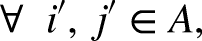
Lastly, to enhance the clarity of the proposed workflow, a roadmap of the major steps involved is shown in Figure 2 using spatial datasets, which may be geological or geophysical data as input. However, note that standardization is needed when using quantitative predictors, and dummy coding is imperative with qualitative predictors in this workflow.

Figure 2.

Our proposed geostatistics-based machine learning workflow for spatial multivariate analog identification of subsurface resources.

Results and discussion

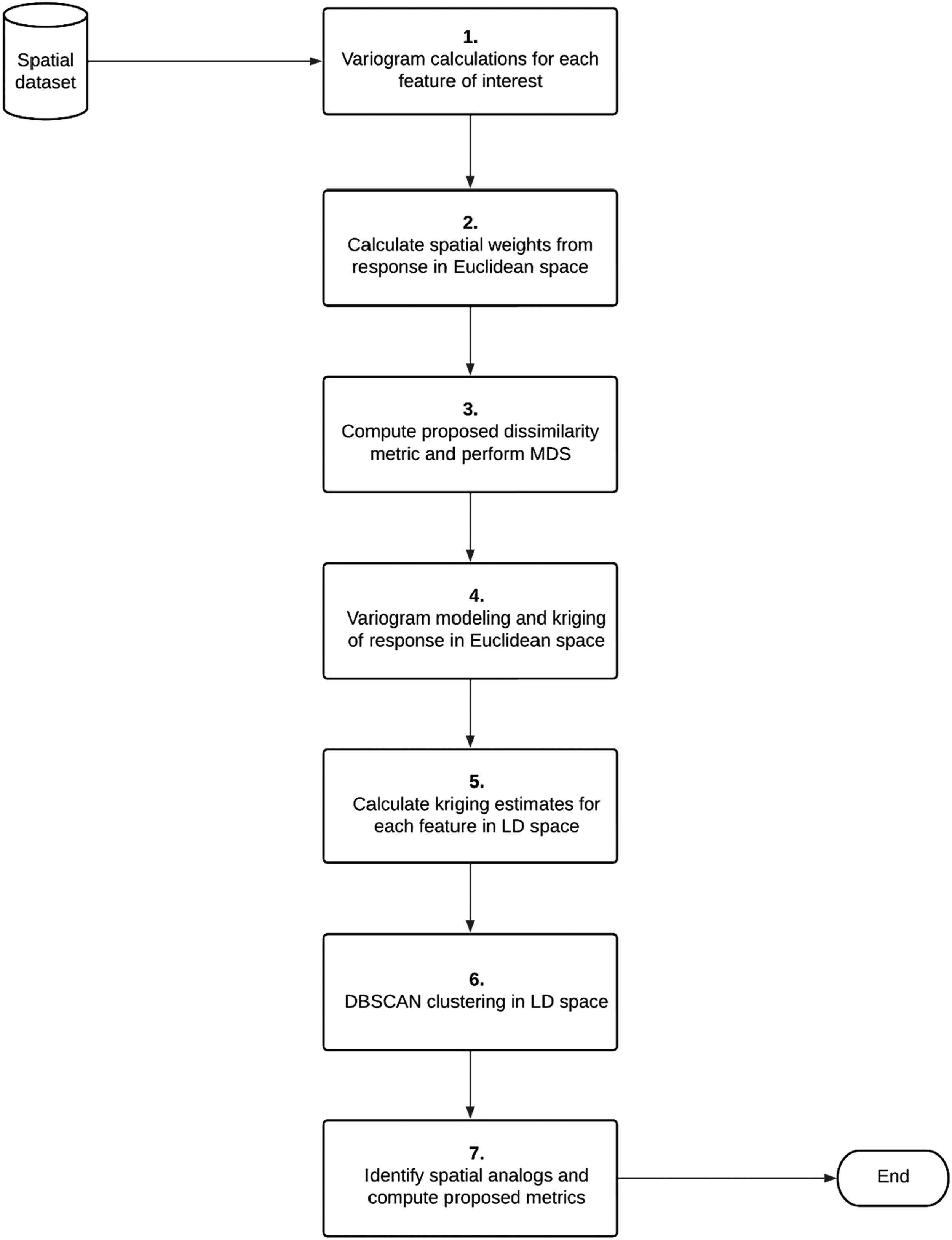
Our proposed workflow is demonstrated for two applications in an oil and gas dataset from the South Kaybob field in the Duvernay Formation. The Duvernay Formation was deposited in a subequatorial epicontinental seaway in the late Devonian–Frasnian time, corresponding to the maximum transgression of the late Devonian Sea into the Western Canadian craton (Figure 3). There exists a series of sub-basins deposits of shale from west to east because of the paleo-lows that include shale in a basin and slope environment. Moreover, mineralogy changes in the west-to-east direction; for instance, the contents of silica and quartz are larger in the west than in the east region. On the contrary, the east region contains larger carbonate and clay content. The formation produces across the entire gas, condensate, and oil windows between 2000 and 3700 m depth. Finally, the predominant hydrocarbon production comes from the western shale basin, specifically from the Kaybob region (Salazar et al., 2023). The first application is an introduction that analyzes a subsurface dataset curated after feature selection and has a sample size of $55$ wells consisting of petrophysical and geological features as predictors. The predictors are porosity (fraction), thickness (km), pore pressure (MPa), oil saturation (fraction), and a response feature of cumulative gas produced (MMscf) over a northeast location vector. The second application adds extreme well cases in the analysis: infill, outlier, centered, and sparse wells for testing. In addition, a summary statistics table showing the data scope of the response and predictor features for the subsurface dataset used is shown in Table 1. For all geostatistical analysis, Python's GeostatsPy package (Pyrcz et al., 2021) is used to re-implement the GSLIB program in FORTRAN (Deutsch and Journel, 1998).

Figure 3.

Input from the geological and geophysical wells colored in red, alongside horizontal producers colored in green within the Duvernay Formation.

Table 1.

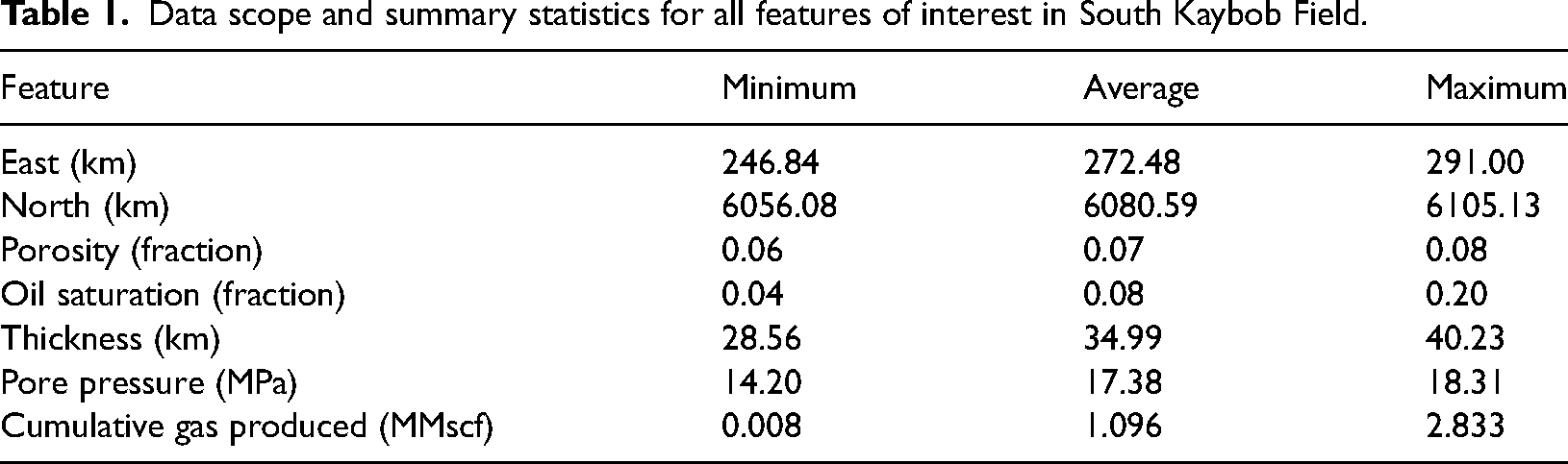
Data scope and summary statistics for all features of interest in South Kaybob Field.

Feature	Minimum	Average	Maximum
East (km)	246.84	272.48	291.00
North (km)	6056.08	6080.59	6105.13
Porosity (fraction)	0.06	0.07	0.08
Oil saturation (fraction)	0.04	0.08	0.20
Thickness (km)	28.56	34.99	40.23
Pore pressure (MPa)	14.20	17.38	18.31
Cumulative gas produced (MMscf)	0.008	1.096	2.833

Workflow demonstration

Variogram modeling is performed on the response feature, standardized gas cumulative production, to determine the semivariogram and quantify spatial continuity along the major direction in Euclidean space as ${\theta }_{\mathrm{maj}}=113,$ including the major and minor variogram ranges of $h_{\mathrm{maj}}=14\mathrm{km}$ and $h_{\min }=10\mathrm{km}$ in Figure 4. In Figure 4, the variogram model fit to the experimental variogram along the major and minor ranges appears similar because an isotropic azimuth tolerance of $90\circ$ is used for all lag distance pairs. The spatial weights from the variogram model almost equally account for the spatial and multivariate contributions of the data pairs over varying lag distances. Recall that the proposed dissimilarity metric combines spatially weighted Euclidean and spatially modified Mahalanobis distances. The spatial dissimilarity metric is determined using the well locations in the east and north, while the multivariate dissimilarity metric is estimated using normalized predictor features. Next, the dissimilarity matrices are sorted using a hierarchical agglomerative clustering method with Ward linkage to enable the visualization of inherent groupings indicative of clustering within the data. For example, Figure 5 highlights that using the spatially weighted Euclidean dissimilarity matrix (weighted close-ology) and the spatially weighted Mahalanobis dissimilarity matrix (weighted multivariate analysis) will tentatively have 5 and 3 groupings, respectively. Meanwhile, combining these dissimilarity matrices as the proposed method tentatively results in $4$ groupings.

Figure 4.

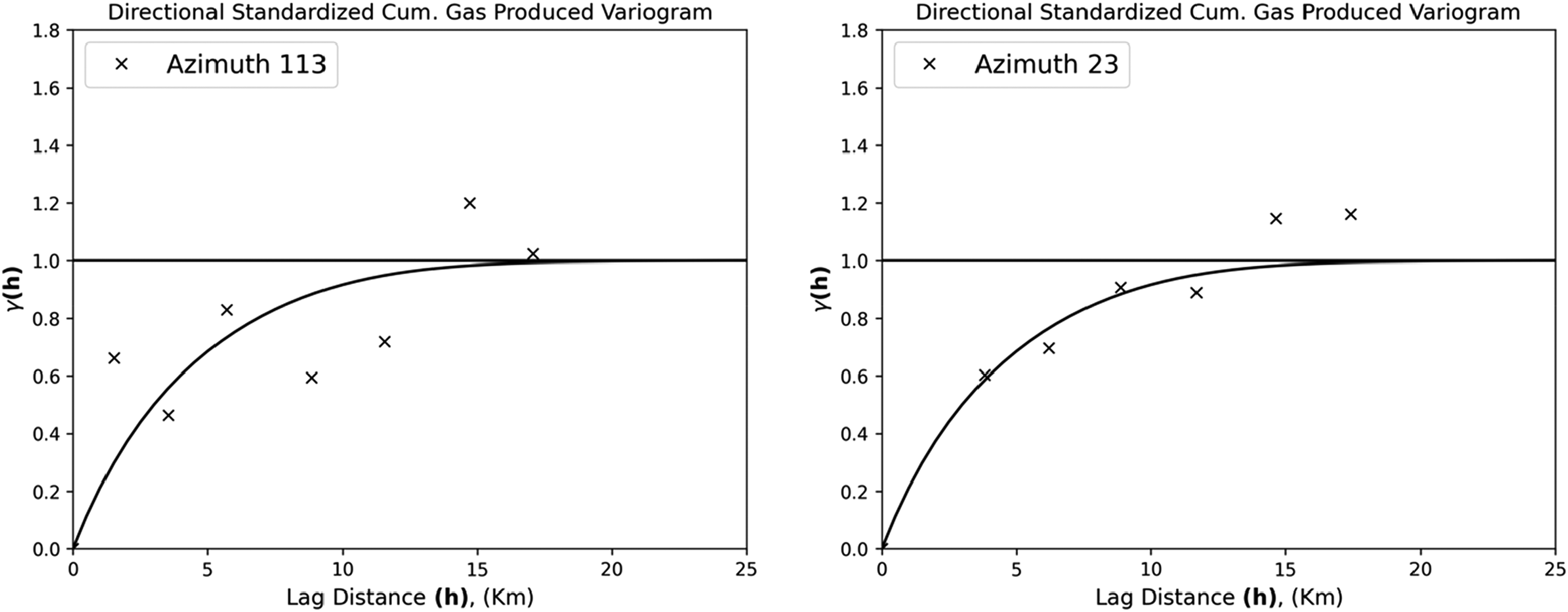
Variogram model of standardized cumulative gas production in Euclidean space. Left: the major direction of spatial continuity and right: minor direction of spatial continuity.

Figure 5.

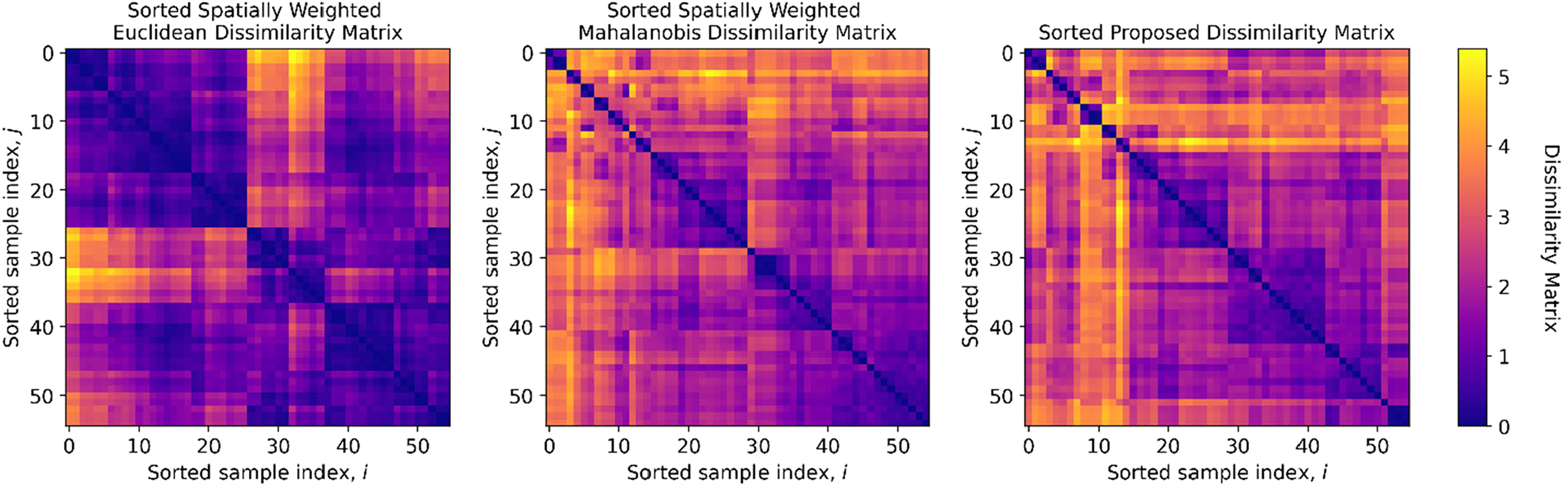
Sorted dissimilarity matrices. Left: proportion of dissimilarity matrix attributed to spatial contribution from Euclidean space. Center: proportion of dissimilarity matrix stemming from all predictors in the multivariate feature space. Right: combined dissimilarity matrix proposed to account for both spatial and multivariate feature space contributions.

Using our proposed spatial multivariate dissimilarity matrix, metric MDS projects the samples to a reduced dimensionality with $X^{\mathrm{\prime }}=\mathrm{MDS}1$ and $Y^{\mathrm{\prime }}=\mathrm{MDS}2$ . Performing variogram modeling on standardized cumulative gas produced to describe the directions of spatial continuity in the MDS space yields a major and minor range of $h_{\mathrm{maj}}=0.4$ and $h_{\min }=0.19$ , respectively, at ${\theta }_{\mathrm{maj}}=55$ . With the Euclidean and MDS space cumulative gas production variograms, kriged estimation maps are obtained and visualized with the well samples in Figure 6. Figure 6 shows cumulative gas production has a slight north-eastern trend with isolated increases in the Euclidean space and north-western trend in MDS space.

Figure 6.

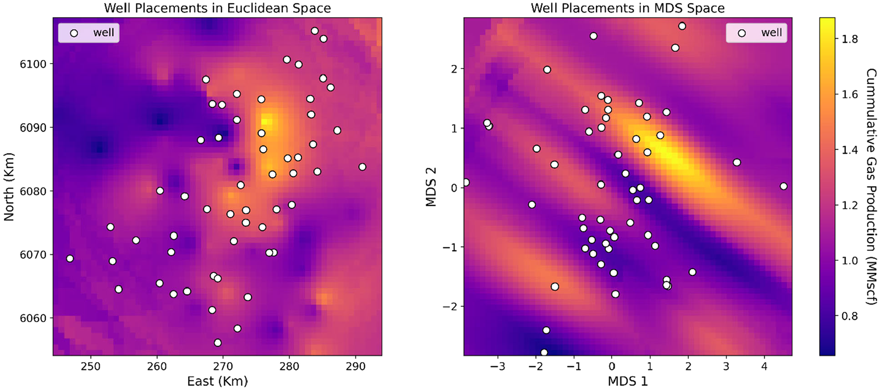
Kriged cumulative gas production maps with data samples. Left: Euclidean space and right: multidimensional scaling (MDS) space of reduced dimensionality.

The direction of spatial continuity for each predictor feature in Table 2, variogram modeling, and ordinary kriging estimates for all predictors in the MDS space are applied to calculate feature trend maps. For example, the trend map in Figure 7 shows porosity has an increasing north-western trend similar to gas production while oil saturation, thickness, and pore pressure have a decreasing north-eastern trend.

Figure 7.

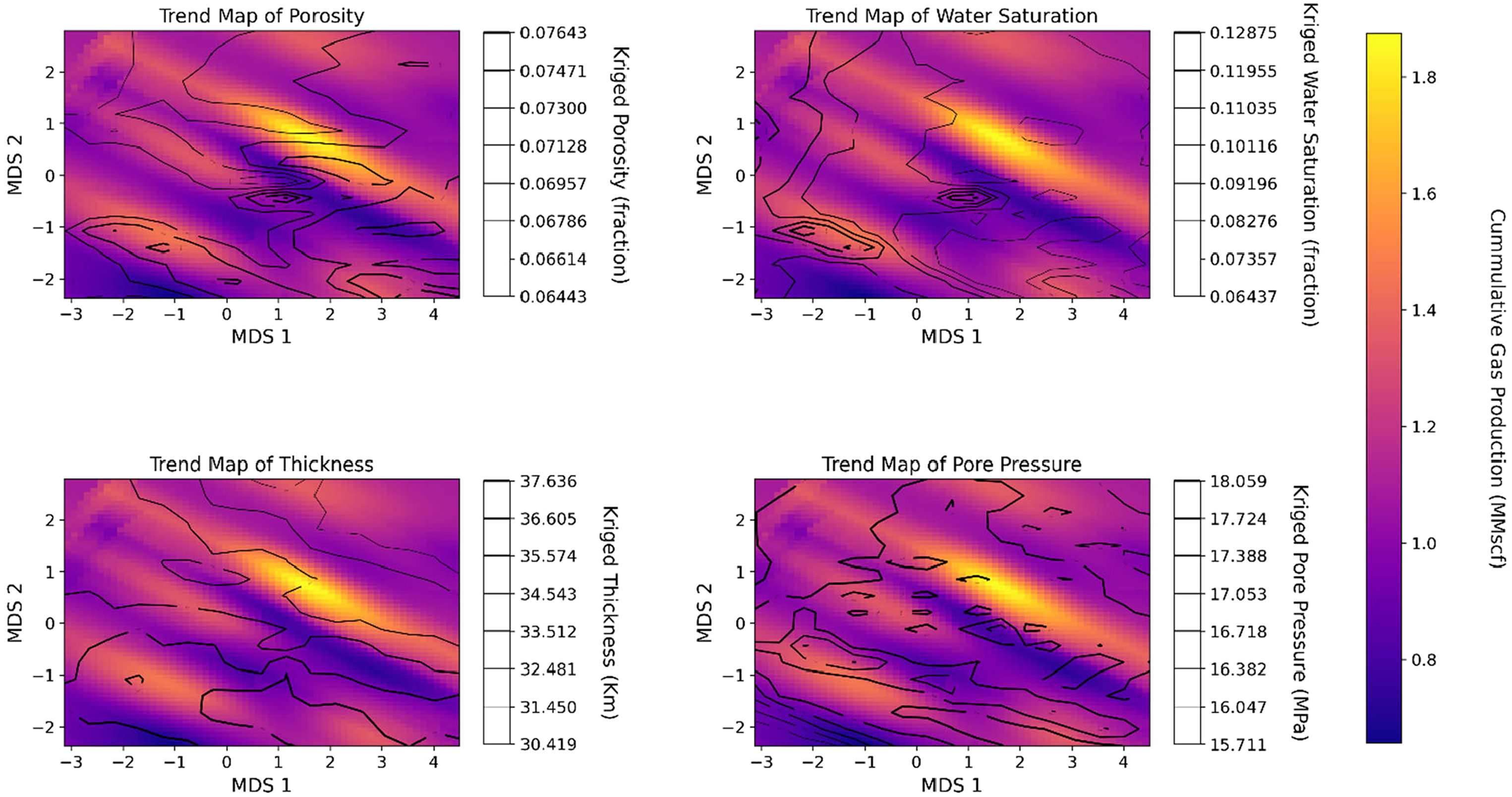
Trend map of kriged estimates for all predictors in MDS space as contour lines for productivity exploration and diagnostics, where increasing line width indicates an increase in magnitude and vice versa. This is underlaid by the map of kriged gas production estimates in the MDS space to extract information from two bivariate distributions. MDS: multidimensional scaling.

Table 2.

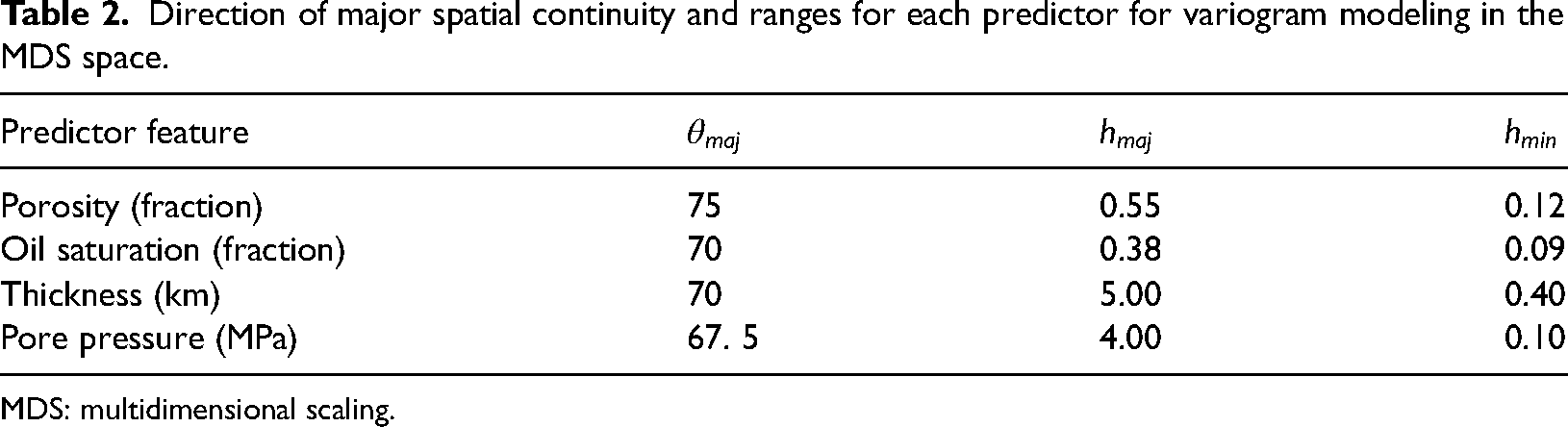
Direction of major spatial continuity and ranges for each predictor for variogram modeling in the MDS space.

Predictor feature	${\theta }_{maj}$	$h_{maj}$	$h_{min}$
Porosity (fraction)	75	0.55	0.12
Oil saturation (fraction)	70	0.38	0.09
Thickness (km)	70	5.00	0.40
Pore pressure (MPa)	67. 5	4.00	0.10

MDS: multidimensional scaling.

Combining all predictor trends with the cumulative gas production trend, possible new well locations and well diagnostics are identified, such as samples or regions with high or low productivity.

Next, the average intersample distance between well samples determined by the nearest neighbor (elbow method) using normalized MDS projections is 0.059. However, since the data is clustered on a small scale, as shown in the elbow plot from Figure 8, it is inadequate to use the intersample distance as the radius parameter, $\epsilon$ , in DBSCAN. Performing hyperparameter tuning on $\epsilon ,\mathrm{\forall }\epsilon =[0.04,0.10]$ depicted by the red rectangle in the MDS space yields an optimal parameter of $\epsilon =0.0729$ at a maximal Silhouette score of $0.15$ and minimum number of points, $n_{pts}=3$ . Using the tuned DBSCAN parameters, $4$ clusters are identified in Figure 9.

Figure 8.

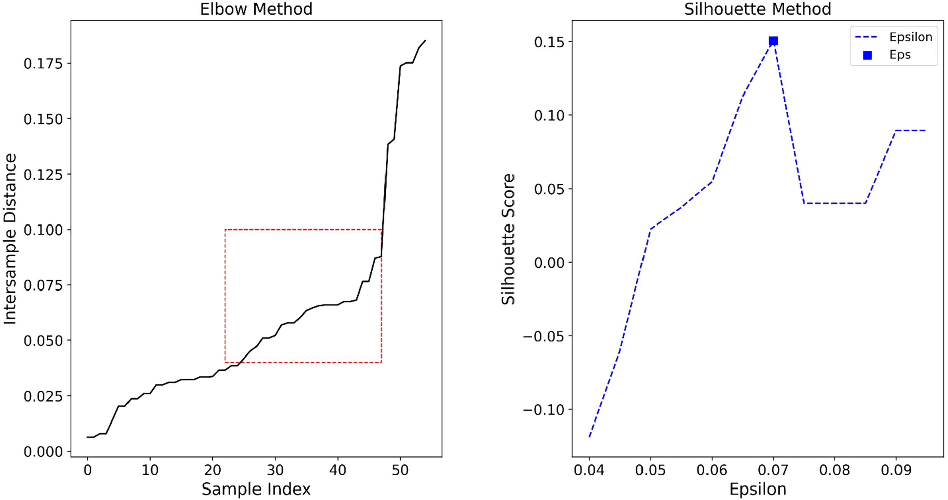
DBSCAN tuning to find optimal parameters in MDS space. Left: $\epsilon$ parameter tuning over a range of values from nearest neighbors (elbow method). Right: identification of optimally tuned $\epsilon$ from silhouette scores. The red rectangle on the left represents the range of $\epsilon$ values used for tuning because there is no distinct elbow. MDS: multidimensional scaling.

Figure 9.

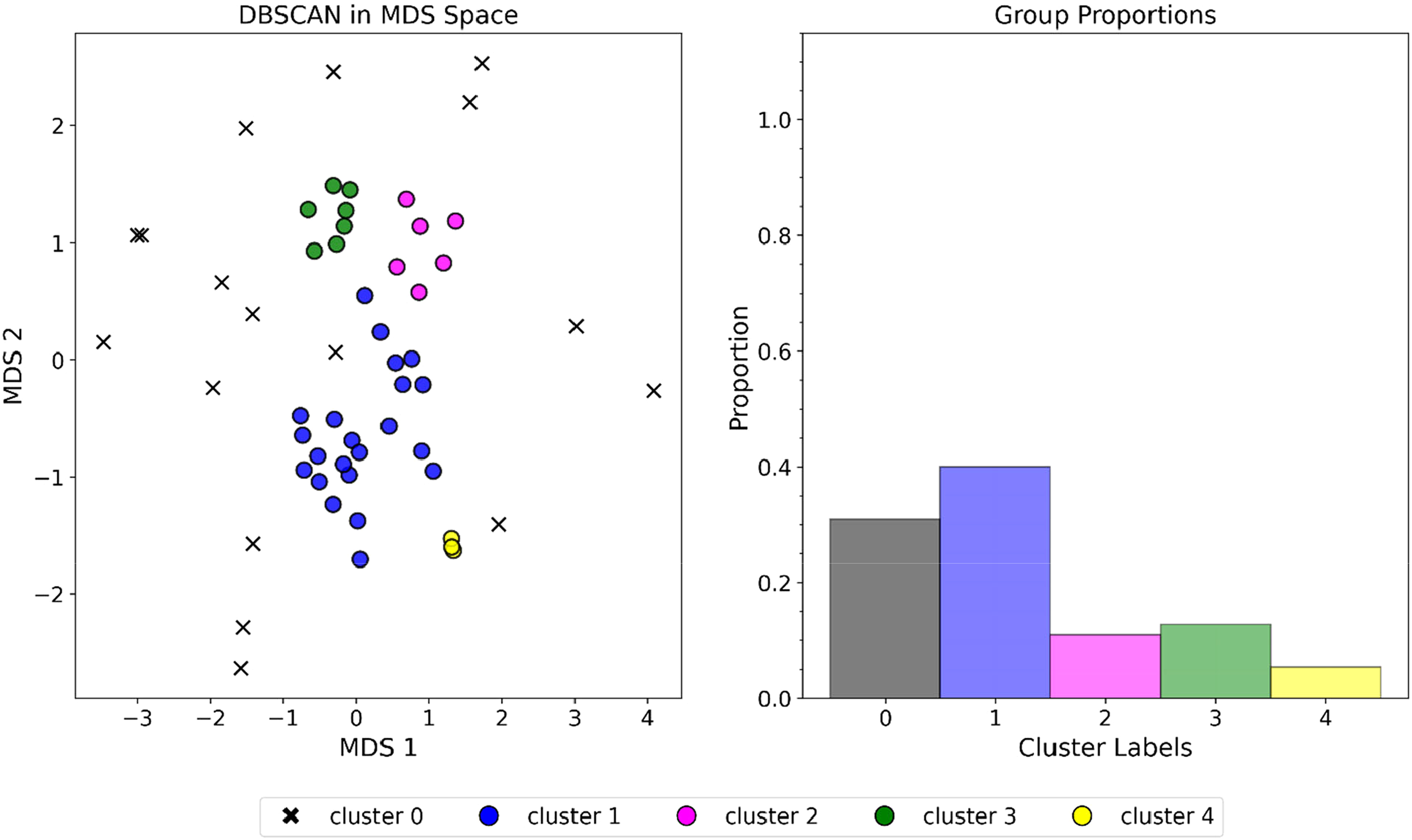
Cluster assignments with DBSCAN in MDS space. Left to right, DBSCAN identification of 4 clusters and cluster proportions. Where cluster 0 represents the DBSCAN outlier label in the MDS space. MDS: multidimensional scaling.

The four combined spatial multivariate clusters identified by DBSCAN indicate that wells within a cluster make a good pool via its respective spatial analogs in the MDS space. Centroid values are assigned to illustrate the separation of analog clusters in Figure 10 to communicate these spatial analogs in the MDS space. For example, observing the MDS space, cluster 1 belongs to a region of wells with relatively low production, while clusters 2 and 3 are in regions of high cumulative gas production, and cluster 4 is in the moderately low production region. Lastly, the cluster labels are used to color-code the well samples by index in the Euclidean space for inferential geological and geophysical well typing.

Figure 10.

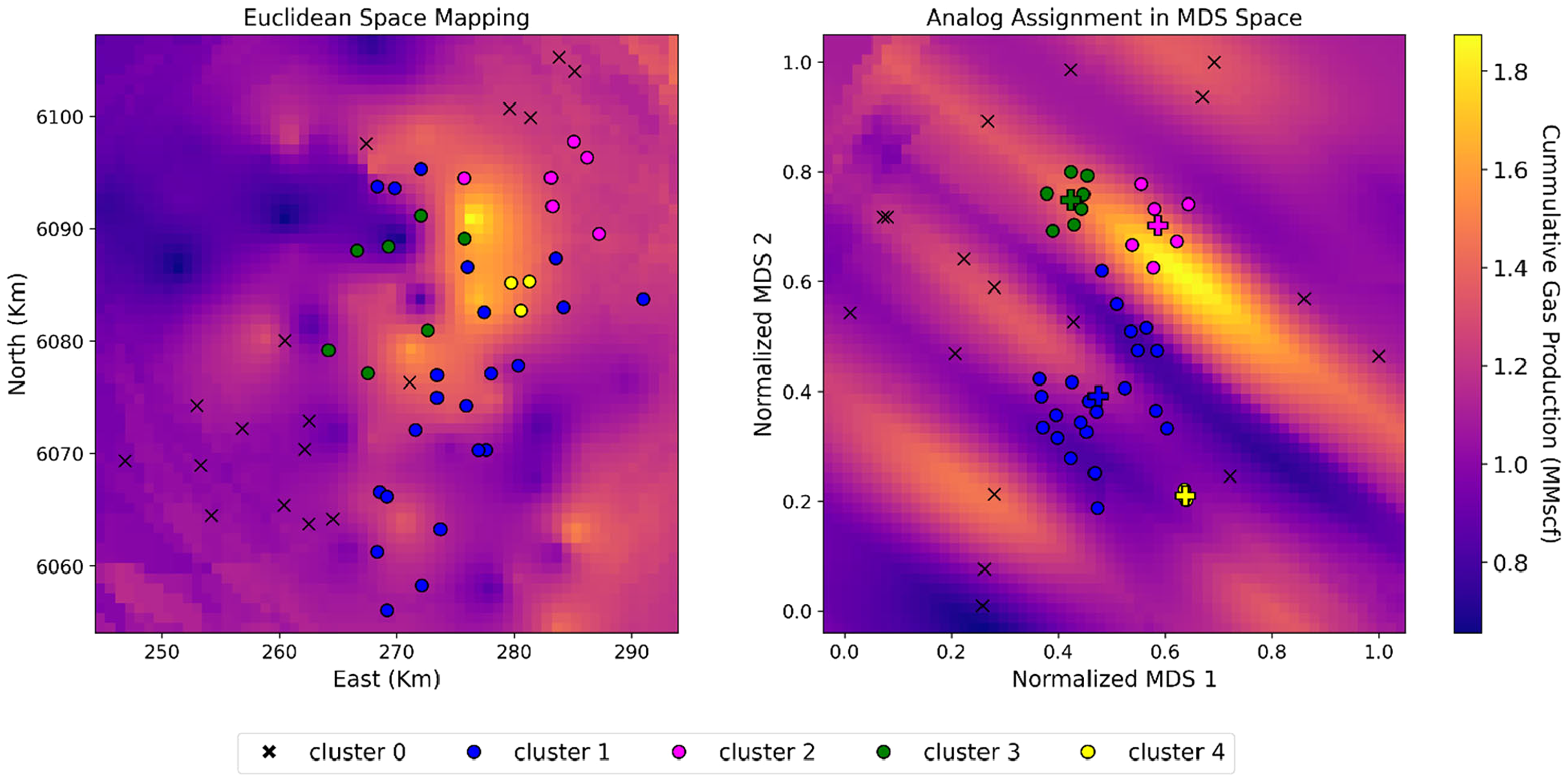
Kriged cumulative gas production maps with data samples. Left: Euclidean space. Right: MDS space of reduced dimensionality with cluster 0 representing the DBSCAN outlier label. Where the cross markers and cluster 0 respectively represent the spatial analogs and DBSCAN outlier label from MDS space. MDS: multidimensional scaling.

Case study with end member test wells

The demonstrated workflow is repeated with extreme cases of samples added in, representing four test wells typically encountered in oil and gas reservoirs: infill, outlier, centered, and sparse wells to ascertain efficacy and stress-test end member wells. In subsequent mentions, these wells are denoted by the letters i, o, c, and s. The proposed workflow is compared to existing methods for analog selection, such as close-ology and multivariate analysis, which computes $\mathit{D}$ using classical Euclidean and Mahalanobis dissimilarity metrics, respectively. Similar to the first application, the variogram model required to compute $\gamma ({\mathrm{h}}_{i,j})$ has a direction of spatial continuity for cumulative gas production at ${\theta }_{\mathrm{maj}}=157.5$ in Euclidean space with $h_{\mathrm{maj}}=22\mathrm{km}$ and $h_{\min }=4\mathrm{km}$ .

Similarly, the spatial continuity in the MDS space for cumulative gas produced is characterized by a major and minor range of $h_{\mathrm{maj}}=0.4$ and $h_{\min }=0.05$ respectively, at ${\theta }_{\mathrm{maj}}=100$ . Using the variogram models calculated for cumulative gas production in both Euclidean and MDS spaces, kriged estimates obtained are visualized with the $59$ well samples. Figure 11 highlights that cumulative gas production has an increasing north-eastern trend in the Euclidean space. Meanwhile, the gas production in the MDS space has an alternate increasing and decreasing laminated north-eastern trend. Recall that close-ology is the grouping by proximity in Euclidean space that focuses on the data's spatial contributions. At the same time, multivariate analysis is the grouping by proximity in the multivariate feature space focusing on the multivariate contributions where these groupings are performed via DBSCAN. Our proposed workflow automatically simultaneously accounts for the combined effects of spatial and multivariate contributions in subsurface datasets during analog identification of subsurface resources. Thus, as discussed in the methodology section, reverting to either close-ology or multivariate analysis on either extremity. Tuning the DBSCAN parameters for the close-ology, multivariate, and proposed cases, but not shown for brevity. Table 3 shows the average intersample distance for all well samples determined by the nearest neighbor (elbow method) as the initial $\epsilon$ and the tuned optimal $\epsilon$ obtained at maximal Silhouette scores for each case with its respective $n_{pts}$ .

Figure 11.

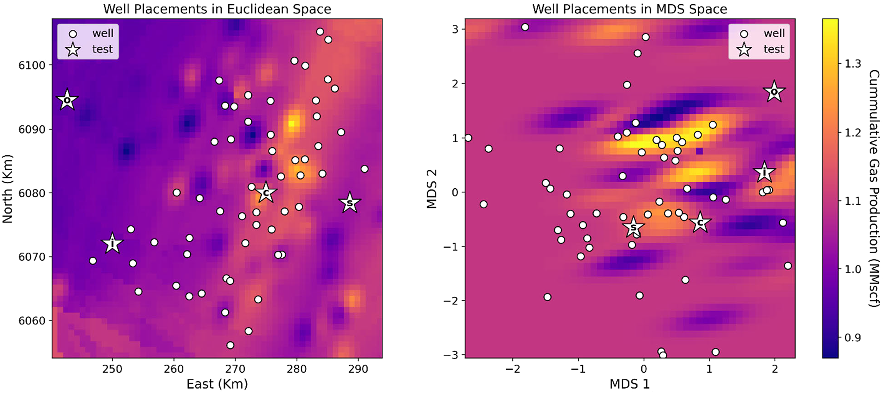
Kriged cumulative gas production maps with data samples, including the 4 test wells. Left: Euclidean space. Right: MDS space of reduced dimensionality. Where the annotated stars i, o, c, and s are the infill, outlier, centered, and sparse test wells, respectively. MDS: multidimensional scaling.

Table 3.

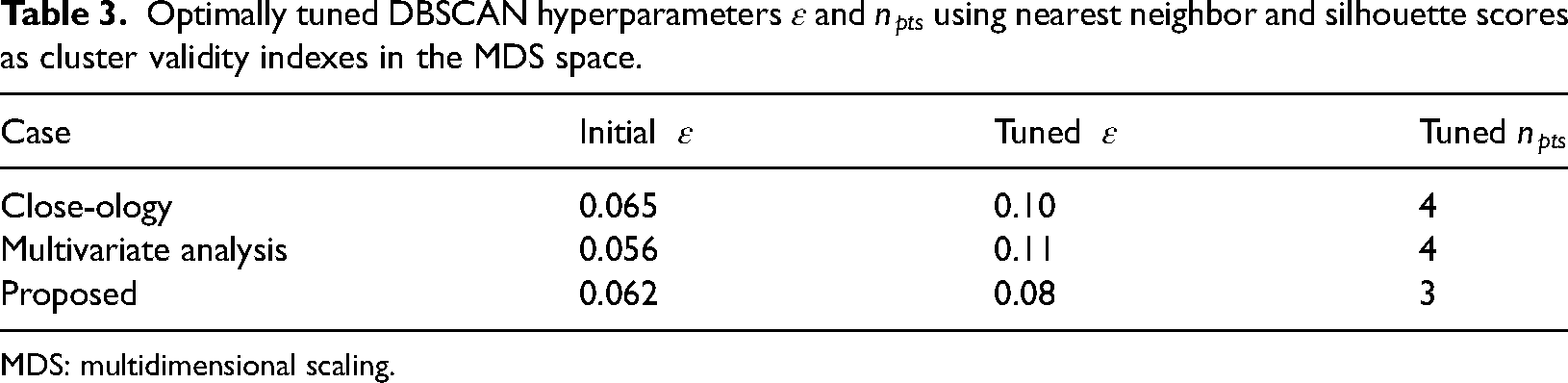
Optimally tuned DBSCAN hyperparameters $\epsilon$ and $n_{pts}$ using nearest neighbor and silhouette scores as cluster validity indexes in the MDS space.

Case	Initial $\epsilon$	Tuned $\epsilon$	Tuned $n_{pts}$
Close-ology	0.065	0.10	4
Multivariate analysis	0.056	0.11	4
Proposed	0.062	0.08	3

MDS: multidimensional scaling.

Using the optimally tuned DBSCAN parameters, four clusters are identified in the close-ology case. In comparison, 2 and 4 clusters were found in the multivariate analysis and our proposed cases, respectively, in Figure 12. However, since DBSCAN clustering is only performed in Euclidean space for the close-ology case using X, Y, it is not possible to generate a map in the MDS space unlike the multivariate and proposed cases with a mappable MDS space.

Figure 12.

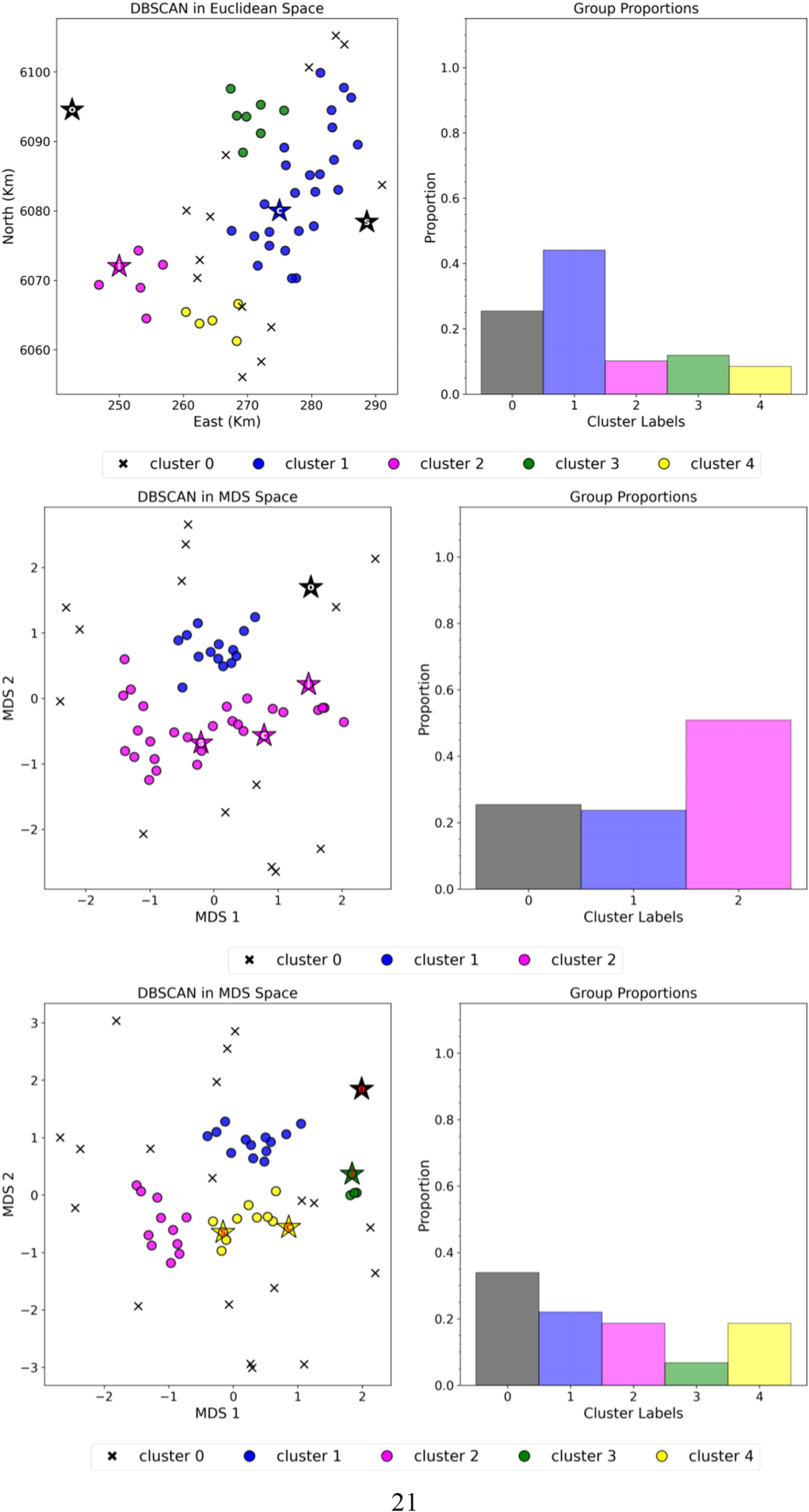
DBSCAN clustering results for the three cases. Top: Close-ology case using classical Euclidean dissimilarity metric for $\mathit{D}$ computation in Euclidean space. Center: multivariate case using classical Mahalanobis dissimilarity metric for estimating $\mathit{D}$ in MDS space. Bottom: proposed case using the novel spatially weighted dissimilarity matrix in MDS space. Where the annotated stars i, o, c, and s are the infill, outlier, centered, and sparse test wells, respectively. MDS: multidimensional scaling.

When metric MDS is computed with different dissimilarity matrix inputs, different LD projections are obtained for the multivariate analysis and proposed cases shown in Figure 13. For these individual cases, 2 and 4 spatial analogs are identified in the MDS space, and their analog clusters are used to color code all well samples by index in the Euclidean space for inferential geological and geophysical typing. For the multivariate case in the MDS space in Figure 13, wells in cluster 1 belong to a variable region of relatively low to medium production and a select few in the high production zones. Meanwhile, wells in cluster 2 are in regions of medium cumulative gas production. For the proposed case in the MDS space, wells in cluster 1 belong to regions of high gas production, cluster 2 in a relatively low gas production region, and clusters 3 and 4 in moderately high production regions.

Figure 13.

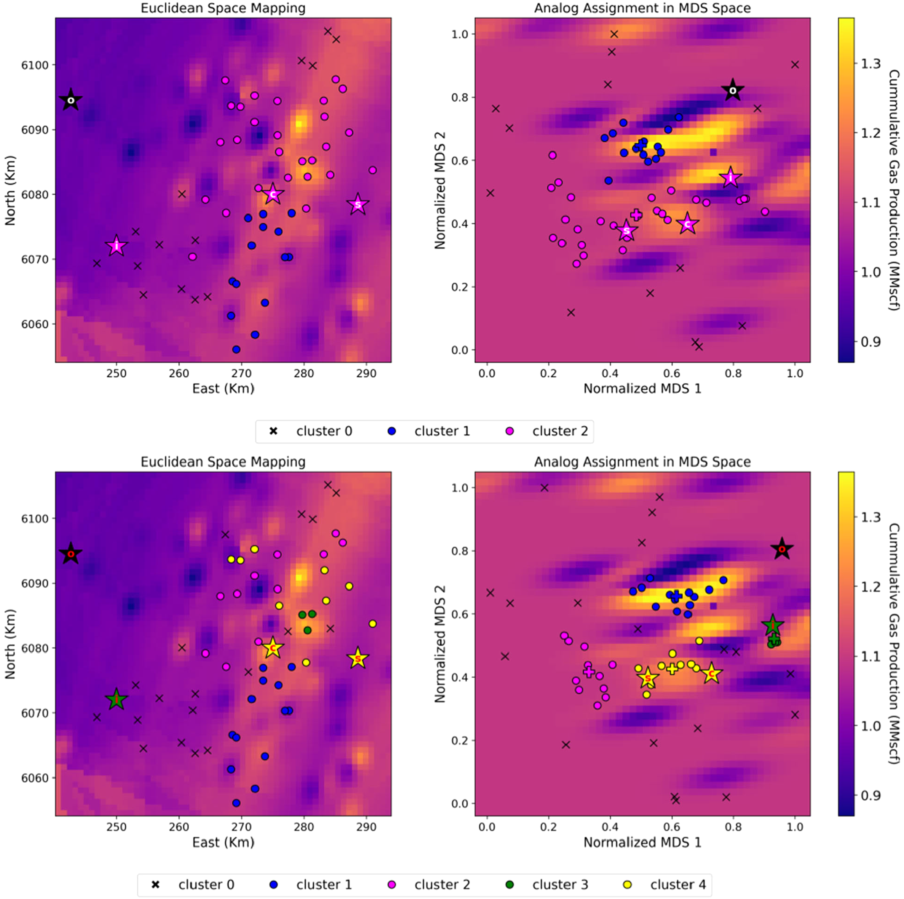
Kriged cumulative gas production maps in Euclidean and MDS spaces with data samples color-coded by cluster labels determined in MDS space. Top: Multivariate case. Bottom: proposed case. Where the cross marker represents the spatial analog in each analog cluster. MDS: multidimensional scaling.

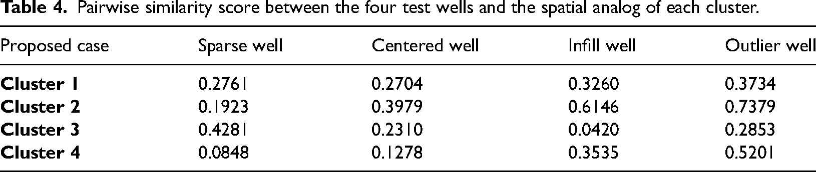
The GCS between each test well and its corresponding spatial analog is determined as 0.0848 for the sparse well in cluster 4, 0.1278 for the centered well in cluster 4, 0.0420 for the infill well in cluster 3, and 0.5270 for the outlier well in cluster 0. Similarly, the PSS between the spatial analog for each analog cluster and the $4$ test wells is estimated in Table 4. Computing the GCS and PSS between the spatial analogs and test wells, notice that the GCS for all test wells except the outlier well is the same as its PSS values because of the combinatorial subset considered. However, the discrepancy between the GCS and PSS scores for the outlier test well at cluster 3 suggests otherwise. This is because comparing the outlier test well to analog clusters may result in inconclusive GCS and PSS results since it is a statistical outlier in either Euclidean or MDS space. A possible limitation of our proposed workflow is its inherent application to mostly mature fields; this ascertains that well samples are sufficient and density reachable such that reliable variogram inference and the DBSCAN clustering are possible.

Table 4.

Pairwise similarity score between the four test wells and the spatial analog of each cluster.

Proposed case	Sparse well	Centered well	Infill well	Outlier well
Cluster 1	0.2761	0.2704	0.3260	0.3734
Cluster 2	0.1923	0.3979	0.6146	0.7379
Cluster 3	0.4281	0.2310	0.0420	0.2853
Cluster 4	0.0848	0.1278	0.3535	0.5201

Conclusions

We introduce a novel workflow for spatial, multivariate analog selection applicable to subsurface resources utilizing geostatistical and machine learning techniques. Our innovative workflow provides a reliable alternative to traditional expert-driven and statistical analog identification workflows, addressing challenges such as the curse of dimensionality, objectivity, repeatability, and accounting for spatial context. The proposed workflow integrates a hybrid dissimilarity metric that simultaneously accounts for both spatial and multivariate contributions of the data and inferential machine learning for dimensionality reduction to flexibly mitigate the curse of dimensionality to cluster analog groups. With the proposed workflow, subsurface resource analogs are identified using this robust and generalizable framework to support inferential analyses and decision making in highly dimensional spatial datasets. The proposed workflow provides an unbiased, repeatable alternative to support conventional expert-driven workflows in contrast to existing methodologies such as close-ology and multivariate analysis. Our workflow requires sufficient data for reliable variogram and density-based clustering model inferences, along with associated assumptions such as stationarity of the variance, variogram, and clustering scale. Nonetheless, this study paves the way for future research, offering a framework that can be optimized and adapted to various datasets, ultimately contributing to developing advanced analog selection tools.