Sage Journals: Discover world-class research

Abstract

In this article, the performance of a 3.36 kWp grid-connected photovoltaic system (GCPVS) under warm and subhumid weather conditions and the development of a predictive mathematical model is presented. Climate data of the 2021 year were used to evaluate energy generation, different types of performance, and efficiency. The average annual yield, corrected yield, array, and final yields were 6.45 h/day, 6.18 h/day, 5.16 h/day, and 4.97 h/day, respectively. The overall annual mean capacity factor and efficiency ratios were 20.73% and 77.22%, correspondingly. Experimental data were analyzed and correlated by multivariate linear regression (MLR) prediction and simulation to validate models. The MLR analysis showed that the efficiency is highly dependent on the temperature of the PV modules and that climatic parameters significantly affect the efficiency and output electric power. The prediction models for PV module efficiency, system efficiency, and direct current energy exhibit an uncertainty of ±1.04%, ±0.57%, and ±35.38 kWh, one-to-one. The monthly generation was compared with results obtained by Energy3D simulation-free software, showing an absolute error of ±2.33 kWh. This information can be used as a methodological tool for predicting efficiency and power generation in direct current.

Graphical abstract

This is a visual representation of the abstract.

Keywords

Grid-connected photovoltaic system GCPVS PVS performance PVS efficiency multivariate regression analysis Energy3D

Introduction

In recent decades, global energy demand has become one of the most important challenges facing humanity. In 2021, the energy consulting and intelligence company reported that the total primary energy supply in the world reached 14,646 Mtoe (million tons of oil equivalent), of which 29% comes from oil, 27% from coal, and 24% from gas, while 10% from biomass and the other 10% is obtained from resources such as hydropower, nuclear, solar, wind, geothermal, etc. (Enerdata, 2021). The over-exploitation of fossil fuels by human activity has led to a rapid decline in fossil fuel reserves. In addition, air pollution, acid precipitation, global warming, and climate change are currently the most severe global environmental problems that require a solution to avoid an environmental crisis in the near future (Gielen et al., 2019). Among the strategies to protect the environment is the use and generation of energy through renewable energy resources to reduce dependence on oil and the decreasing availability of hydrocarbons. According to the Secretaría Nacional de Energía (SENER, by its Spanish acronym), México is a country highly dependent on fossil fuels. In the first half of 2018, 75.88% of the national primary energy generation has its origin from hydrocarbons and 17.29% from renewable sources (SENER, 2018). However, to ensure energy supply in México, the government established changes in policies, laws, and regulations through the Energy Reform. This reform aims to change the model based on fossil fuels toward clean energies. In particular, one of the complementary energetic laws: the Energy Transition Law (SENER, 2017) previously published (2015), whose main objective is to regulate the sustainability of energy generation and gradually increase the use of clean energy by 2024, up to 35%; additionally, it is expected that the law will contribute to reduce polluting emissions from burning fossil fuels. In México, the use and promotion of renewable energies is focused not only on reducing environmental impact, but also opens a new way to create a diversified economic market. The current availability of renewable resources and further development of wind and solar energy will lead to lower costs in the generation of electricity for domestic and industrial use. According to SENER data, México has a great deal of potential for electricity generation through renewable sources, with an installed capacity in 2020 of 212,033.33 GWh (763.32 PJ) which includes solar, wind, geothermal, hydro, and biomass energy. In México, the demand for photovoltaic systems (PVS) has recently increased, reaching an installed capacity of solar energy in grid-connected photovoltaic systems (GCPVS) reaching 1388 MW in 2020 (SENER, 2020). Local climatic conditions and PV components represent an important factor in the generation of quality electrical power from GCPVS. In recent years, numerous studies have been carried out on the evaluation of the performance of GCPVS operating under different climatic conditions for residential and industrial applications. Adaramola and Vågnes evaluated the performance of a PVS connected to the grid installed on the roof of a building under local climatic conditions. The study showed that in the summer months, maximum performance is reached, especially in June and July. The data are comparable to the systems installed in the northern region of Europe; however, the PVS suffered losses due to snow and frost (Adarmola and Vågnes, 2015). Similarly, Savvakis and Tsoutsos evaluated the 2-year performance of a 2.18 kWp grid-connected PV system installed at the Technical University of Crete, Chania, in which they observed that the performance depends on the operating temperature of the panel frame (Tm), with increased power generation in the period from June to August, the study revealed that the temperature of the photovoltaic frames is inversely proportional to efficiency (Savvakis and Tsoutsos, 2015). Similarly, Quansah et al. studied performance by comparing five different PVS technologies installed on the roofs of Ghana University of Science and Technology buildings. The research revealed that PVS based on copper indium disulfide (CIS) is the least suitable technology for those climatic conditions, while the PVS with the highest generation performance is heterojunction incorporating thin (HIT) for regional study conditions (Quansah et al., 2017). Also, de Lima et al. analyzed the generation capacity and performance of a 2.2 kWp PV system installed at the State University of Ceará, Brazil, PVS monitoring allowed for determining an average annual capacity factor of 19.2% and an average annual performance ratio of 72.9% (de Lima et al., 2017). In another study, Tahri et al. analyzed GCPVS based on two types of PV module technologies, installed at the National Institute of Advanced Industrial Science and Technology, Japan, under tropical climate conditions, concluding that polycrystalline module technology is the most suitable, achieving higher performance and energy generation in Summer, while CIS technology PV systems, presented higher final performance, particularly in winter (Tahri et al., 2018). Dondariya et al. conducted the study to evaluate the feasibility of a GCPVS installed on the roof of a residential building in India, based on the simulation of photovoltaic performance from a comparative study of equations of a model and climate data to determine the actual PV performance (Dondariya et al., 2018). Al-Badi analyzed the measured results of a 1.4 kWp grid-connected PV plant in desert conditions, where a significant effect was observed by the dust of the region on the PVMs, reducing up to 10% in energy generation and efficiency (Al-Badi, 2018). Akpolat et al. present an overview of Turkey's potential situation and a simulation study for the design and calculation of the Rooftop Solar Photovoltaic System (RSPS) for the Marmara University Faculty building in Istanbul (Akoplat et al., 2019). Thotakura et al. analyzed the performance of a MW-scale GCPVS installed in an educational institute in the coastal region of Andhra Pradesh, under humid and dry tropical climatic conditions, performed a comparative study between real-time monitoring and parameter simulation, with the yield ratio of the solar photovoltaic plant at over 80%, covering approximately 20% of campus energy consumption (Thotakura et al., 2020). Finally, Akhter et al. studied the performance of a GCPVS based on three PV technologies in the tropical climate, together with a composite PV system installed on the engineering tower of the University of Malaya, Malaysia, with polycrystalline silicon (p-Si) PVM being the highest performing compared to monocrystalline (m-Si) and amorphous silicon thin film (a-Si), with an average maximum efficiency of 12.17% (Akhter et al., 2020).

The contribution of this research consists of the study and analysis of a GCPVS in warm/subhumid climatic conditions, including the development and empirical validation of a prediction model based on multivariate linear regression (MLR) analysis and computer simulation. These results can be guides for similar applications in which researchers and engineers can predict the performance of this kind of PVS since there is a limited technical background of solar photovoltaic resources applied to the utilization of grid-connected systems under similar climatic conditions. In addition, the performance data collected can provide useful information for university campuses and policymakers where sustainable construction and clean energy generation is a goal, ensuring a degree of reliability in their PV installations.

Materials and methods

PVS description

Table 1 shows the characteristics of the system consisting of polycrystalline silicon Kyocera modules (KD240GX-LFB model). The electrical and climatological parameters were recorded by a communication portal (SMA brand Sunny Web Box) using sensors in ten-minute periods, such as (1) global insolation, (2) wind speed, (3) ambient temperature, (4) PV module temperature, (5) alternating current energy, and (6) direct current energy.

Table 1.

PVS details.

Parameter	Specification
Cell technology PV module	Polycrystalline silicon
Module efficiency	14.50%
Cell efficiency	16.00%
Maximum power	240 W
Maximum system voltage	1000 V
Voltage at maximum power	29.8 V
Current at maximum power	8.06 A
Open circuit voltage (V_oc)	36.9 V
Short circuit current (I_sc)	8.59 A
Temperature coefficient at Pmax.	−0.46% / K
Number of modules	14
Module area	1.64 m²
NOCT	45 °C

GCPVS performance analysis

Electrical energy generation is the amount of alternating current (AC) and direct current (DC) produced by the PVS in a given time. The total electrical energy produced can be hourly, daily, or monthly, and is determined from the following sections (Adarmola and Vågnes, 2015; Savvakis and Tsoutsos, 2015; Quansah et al., 2017).

Direct current electrical energy, E_DC

The amount of energy generated by the PVS or net energy of the photovoltaic modules, at a time, t, is expressed in terms of power, current intensity, and voltage, P, I, V, respectively, see Equation (1).

E_{D C 2} = a + b T_{P V} + c G_{i} + d v - e T

(1)

The daily electrical energy generated by the PVS is determined by Equation (2), and the monthly energy is determined by the sum of the daily energy multiplied by the days of the month under study (Savvakis and Tsoutsos, 2015).

E_{D C . d} = \sum_{t = 0}^{t = 23} V_{D C} I_{D C} t

(2)

Alternating current electrical energy, E_AC

It represents the energy output or net energy of the inverter, expressed in terms of electrical power, current intensity, and voltage; see Equation (3), while the total daily and monthly alternating current energy is determined as shown in Equation (4), where N represents the number of days in the month under study. To determine the active energy, the term cos(Φ) is included, where Φ is the phase angle between the electrical voltage and current signals, V_AC and I_AC, respectively; and the monthly energy is determined by the sum of the daily AC energy multiplied by the days of the month under study.

E_{A C} = P_{A C} t \cos ϕ = I_{A C} V_{A C} \cos ϕ

(3)

E_{A C . d} = \sum_{t = 0}^{t = 23} V_{A C} I_{A C} t \cos ϕ

(4)

Reference yield, Y_R

It represents the time (h/day) at which the solar radiation must impinge on the PV array at the reference irradiance, I_STC = 1000 W/m², to generate the energy, E_G_, its value depends on the location, orientation, and inclination of the PVS, as well as the weather conditions (Adarmola and Vågnes, 2015; Quansah et al., 2017), see Equation (5).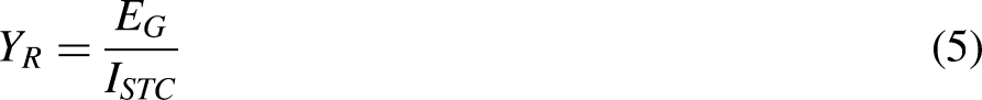

Y_{R} = \frac{E_{G}}{I_{S T C}}

(5)

Pv cell temperature, T_C

The temperature reached by a photovoltaic cell at a given value of ambient temperature, T_amb., and irradiance, G_i, can be determined by Equation (6), where NOCT is the nominal operating temperature of the photovoltaic cell, expressed in °C.

T_{C} = T_{a m b .} + (N O C T - 20) (\frac{G_{i}}{800})

(6)

Corrected reference yield, Y_CR

The corrected reference yield is a correction factor for the module temperature effect and is determined by Equation (7), where α is the PV module temperature coefficient (PVM), T_m is the average PV module temperature, and T_o is the reference temperature (Alshare et al., 2020; Pinheiro et al. 2020).

Y_{C R} = Y_{R} [1 - α (T_{m} - T_{0})]

(7)

Array yield, Y_A

Represents the time measured in h/day that the PV generator must operate at rated power to generate the amount of E_DC power, see Equation (8); that is, the Y_A parameter represents the actual operation of the PV generator in relation to its rated capacity.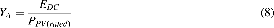

Y_{A} = \frac{E_{D C}}{P_{P V (r a t e d)}}

(8)

Final yield, Y_F

This quantity represents the time, measured in h/day, that the PVS and inverter must be operating at their rated power or capacity, P_PV, to generate E_AC. It reflects the actual operation of the system in relation to its rated capacity, see Equation (9). This parameter depends on the location and type of installation, allowing one to compare different PV systems according to the size and location of a geographical region, as in this case study.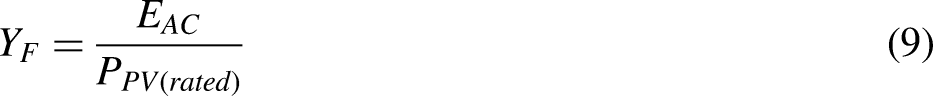

Y_{F} = \frac{E_{A C}}{P_{P V (r a t e d)}}

(9)

Energy losses

The operation of the PV system involves heat transfer by convection and insolation that causes losses that reduce the system’s performance (Savvakis and Tsoutsos, 2015; Quansah et al., 2017). The most important losses are (1) array capture losses, (2) system losses, and (3) overall losses, which are briefly described below.

Array capture losses, L_A

Array capture losses are calculated from the difference between the reference yield and the array yield, a type of loss associated with the variation of the actual insolation with respect to the reference or theoretical insolation.

L_{A} = Y_{R} - Y_{A}

(10)

System losses, L_S

These losses, expressed in h/day, are due to the discontinuous operation of the inverter and are calculated using Equation (11).

L_{S} = Y_{A} - Y_{F}

(11)

Overall losses, L_O

The overall losses are the sum of the PV array collection losses and the system losses, and are determined by Equation (12), also expressed in h/day (Adarmola and Vågnes, 2015).

L_{O} = Y_{A} + Y_{S}

(12)

GCPVS efficiency and performance analysis

PV module efficiency, η_PVM

The instantaneous efficiency of the PV array is given by Equation (13), where E_DC represents the effective energy generated by the module with respect to the available insolation (Quansah et al. 2017). The instantaneous efficiency of the PV array is given by Equation (13), where A_m represents the PVM surface.

η_{P V M} = (\frac{E_{D C}}{A_{m} G_{i}}) (100 %)

(13)

System efficiency, η_sys

The efficiency of the PV system is associated with the balance of systems comprising the PV generator and the power inverter; the instantaneous efficiency of the system can be calculated using Equation (14).

η_{s y s} = \frac{E_{A C}}{A_{m} G_{i}} (100 %)

(14)

Inverter efficiency, η_inv

The efficiency of the inverter depends on its input voltage, the value of which is obtained by Equation (15). Some inverters operate most efficiently in the upper part of the rated electrical power range at maximum power point conditions.

η_{i n v} = \frac{E_{A C}}{E_{D C}} (100 %)

(15)

Performance ratio, PR

It is useful for characterizing the performance of a PVS. The PR is calculated as the ratio between the useful energy generated and the energy that should be generated by an ideal (i.e., lossless) PVS at 25°C receiving the same insolation. The PR parameter does not depend on configuration, size, or location, and allows comparing the generation between different GCPVS. However, this parameter does not allow a direct determination of the causes of losses. Equation (16) shows how to obtain the coefficient of performance of the GCPVS.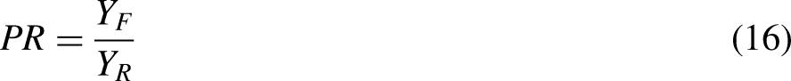

P R = \frac{Y_{F}}{Y_{R}}

(16)

Capacity factor, CF

It is a useful parameter to determine the energy delivered by a GCPVS. The capacity factor is defined as the ratio between the AC power output and the amount of energy of a PV system operating at rated power, considering a correction factor, see Equation (17).

C F = \frac{E_{A C, a n n u a l}}{8760 P_{P V (r a t e d)}}

(17)

Results and discussions

The performance of the PVS was evaluated under real conditions, and a predictive model was developed to compare generation yields and energy efficiency. This section presents and discusses the main results of the climatological and electrical data obtained by the data acquisition system (DAQ) of the GCPVS under study, such as (1) climatological data analysis; (2) electrical energy generation; (3) different system and component performances; (4) energy losses; (5) system and component efficiency; (6) coefficient of performance; (7) capacity factor; and finally, (8) multivariate regression analysis to predict the performance of the GCPVS.

Climatological data analysis

Figure 1 shows the monthly average of in-plane solar irradiance (G_i), ambient temperature (T_amb.), PV module temperature (T_m), and wind speed (v) during the period January to December 2021. All the climatological data were obtained in situ via a SMA brand Sunny Web Box acquisition system located at the roof of the main building of the Universidad Politécnica del Estado de Guerrero, UPEGro. It is observed that during the first quarter the data present fluctuations, especially in wind speed, and to a lesser degree, solar radiation in the plane, PVM temperature, and T_amb_. On the other hand, a relatively constant behavior is observed in the module temperature (53–56°C) despite the fact that the ambient temperature shows significant changes between January and June. The relatively constant behavior of the PVM temperature with respect to the variation of T_amb can be attributed to the convective effect of the wind on the surface of the PVM.

Figure 1.

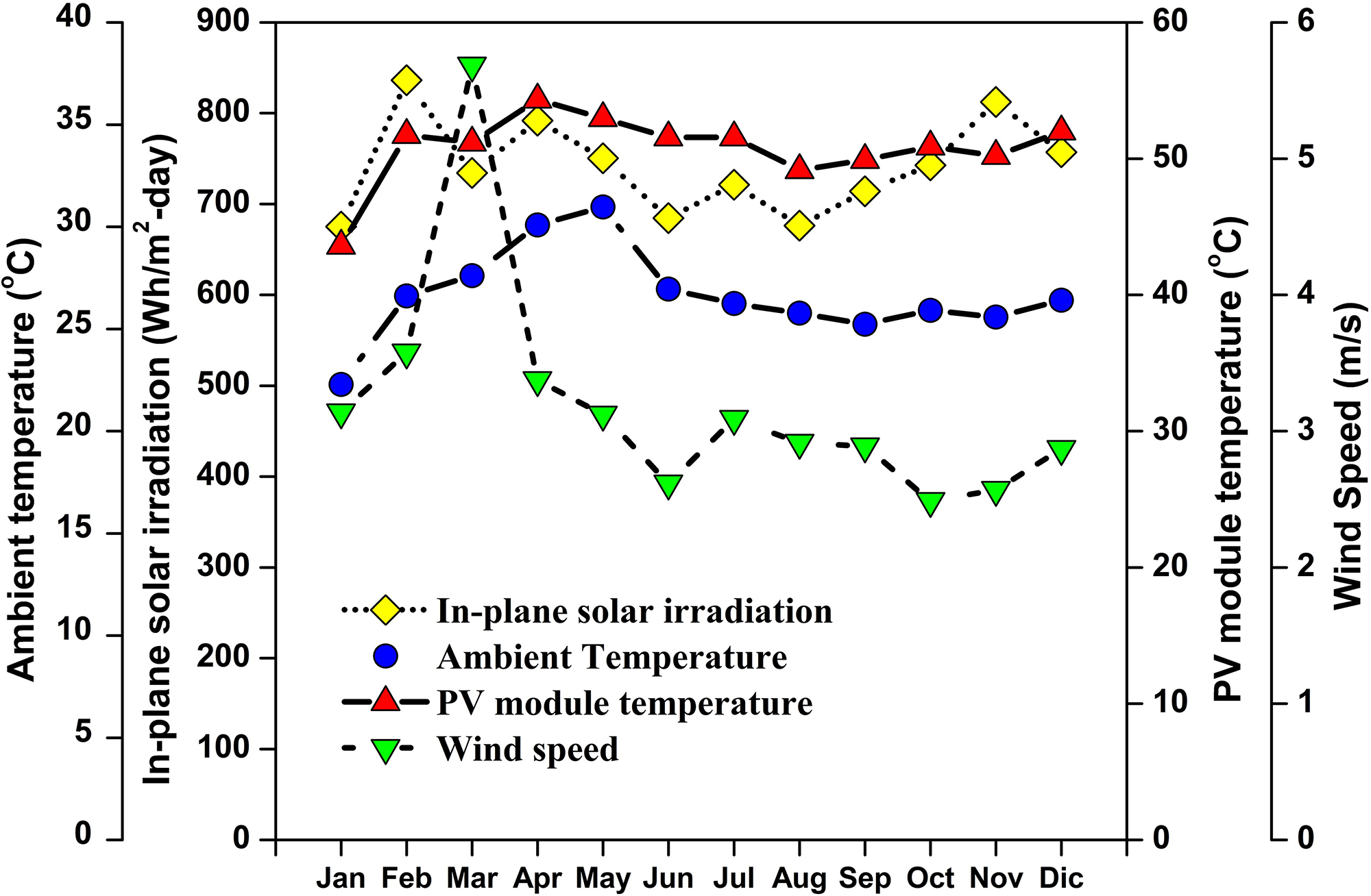
Monthly average value of solar irradiance on the plane, G_i (◇), room temperature, T_amb., (○), PV module temperature, T_m (Δ) and wind speed, v (▽).

The analysis shows that the maximum in-plane solar irradiance of 1104.06 W/m² was recorded in February, with a mean of 836.26 W/m². The lowest ambient temperature (i.e., 15.42°C) was recorded in January, with an average of 23.04°C, while the highest temperature was recorded in May, reaching a temperature of 34.52°C and a mean of 31.54°C. On the other hand, April was the month with the highest PVM monthly mean temperature of 66.51°C, followed by May with 65.18°C. Regarding wind speed, March exhibits the highest mean wind speed value of 6.02 m/s, with a minimum annual value of 3.06 m/s, a maximum of 6.92 m/s. Figure 2 depicts the histogram, normal distribution, statistical mean (µ) and standard deviation (σ) of the statistical analysis of G_i, T_amb., T_m, and v. Figure 2(a) shows the histogram and normal distribution of G_i, with an interval of (400–1100) W/m²day. Figure 2(b) displays the histogram and normal distribution of the T_amb., parameter, 80.44% of the values are in the interval between 14 and 34°C; Figure 2(c) illustrates the histogram and normal distribution of the T_m variable, which have an interval between 45 and 65°C. On the other hand, Figure 2(d) exposed the histogram and normal distribution of the variable v, with 79.08% of the values included in the interval between 2 and 5 m/s. This information gives a general view to understand the data variability, where wind speed shows the lower standard deviation, this statistically means, that wind speed varies from 2.247 to 4.871 m/s (i.e., µ ± σ). Regarding the in plane solar irradiance, it can be observed a negative skewness statistical distribution, a similar case as in the PV module temperature. Finally, it can be observed that all of the climatological data shows a monomodal distribution, showing only one peak.

Figure 2.

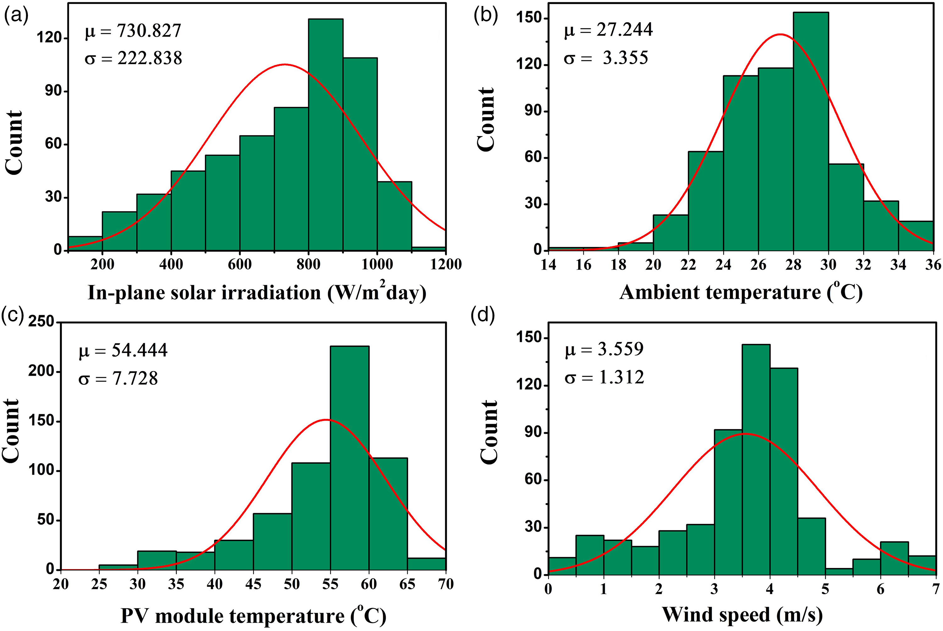
Statistical analysis, histogram, and normal distribution of (a) G_i, (b) T_amb., (c) T_m, and (d) v.

GCPVS output energy

Figure 3 displays the average monthly E_DC generation of the PVS and the cumulative mass of saved CO₂ (which is calculated by the SMA acquisition system) expressed in kg. The average monthly energy supplied by the PV system ranges from 441.77 kWh/month in May to 575.37 kWh/month in July. The annual generation of energy supplied to the grid by the analyzed system is approximately 6347.90 kWh/year, with an average annual generation of 526.45 kWh/month. On the other hand, in Figure 3, it is shown that the average monthly E_DC produced in January is 450.44 kWh/month, corresponding to an average monthly solar insolation of 5.81 kWh/m²day, which is higher than the monthly average in May of 441.77 kWh/month, when a monthly average solar insolation of 6.55 kWh/m²day was recorded, indicating that conditions such as ambient temperature, the PV module's temperature, and wind speed determine GCPVS energy generation, which were analyzed in Climatological data analysis section. Statistical analysis was performed on the E_DC data generated by the PV system. The following parameters were obtained, a population mean µ of 2002.891 kWh/kWp month and a standard deviation σ of 529.742 kWh/kWp month; 86.56% of the values are in the range of (1000 to 2500) kWh/kWp month. The generation of electrical energy by conventional methods produces greenhouse gases, among these gases, mainly CO₂; the use of a PVS contributes to reducing these emissions (Akoplat et al., 2019), the evolution of the amount of kg CO₂ not emitted is quantified as shown in Figure 3. A CO₂ variation of 327.84 kg was observed in May and 433.42 kg in July, with an annual average of 392.91 kg. The EDC parameter varies from 444.91 kW in May to 582.27 kW in July, with an annual average of 565.12 kW, while the total amount of CO₂ avoided annually is approximately 4714.92 kg/year, considering that the consumption habits in an educational institution is similar from one year to another.

Figure 3.

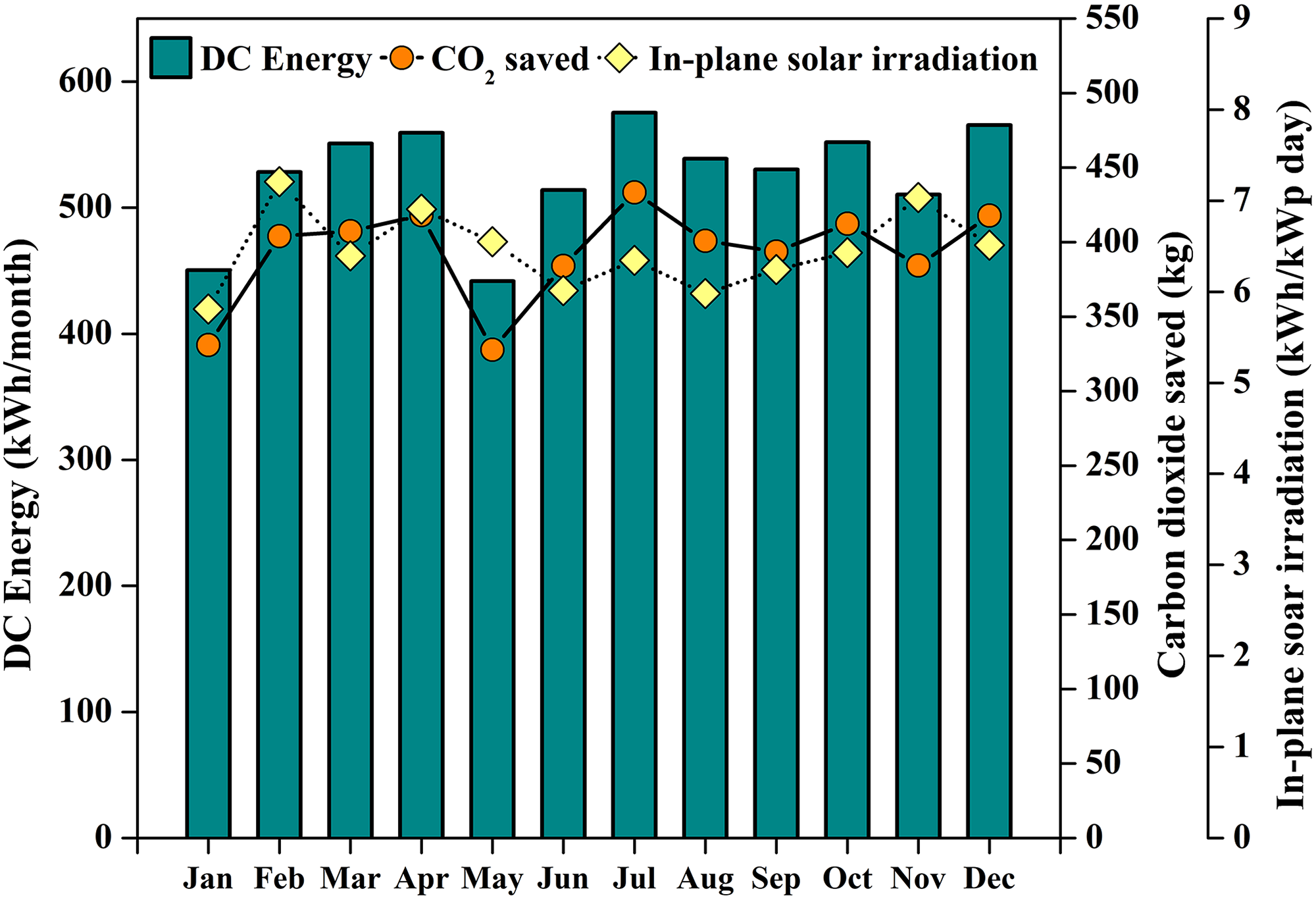
Total energy produced monthly in DC, associated with CO₂ mass savings (○) compared to the in plane solar irradiation (◇).

GCPVS performance types

The monthly average reference yield of the GCPVS ranges from 5.81 h/day in January to 7.21 h/day in February. The range of the obtained corrected reference yield is 5.70 h/day (also expressed as kWh/kWp day) in January and 6.85 h/day in February. The yield of the array is in the range of 4.24–5.62 h/day, in May and February, respectively, and the final yield presents a range between 4.08 h/day in May and 5.40 h/day in July. The annual average of the reference yield, corrected reference yield, array yield, and final yield were 6.45, 6.18, 5.16, and 4.97 h/day, correspondingly. Similarly, the analysis of the standard deviation of the maximum and minimum value of the reference yield in relation to the corrected reference yield, array yield, and final yield (Y_R, Y_CR, Y_A, Y_F) was performed, which shows a minimum of 1.92% in January and a maximum of 4.15% in April, for the corrected reference yield, a minimum of 12.94% in July and a maximum of 35.25% in May; and for the final yield, a minimum of 14.95% in July and a maximum of 37.68% in May; an annual average difference of 2.35%, 19.95%, and 22.78% individually is observed, see Figure 4.

Figure 4.

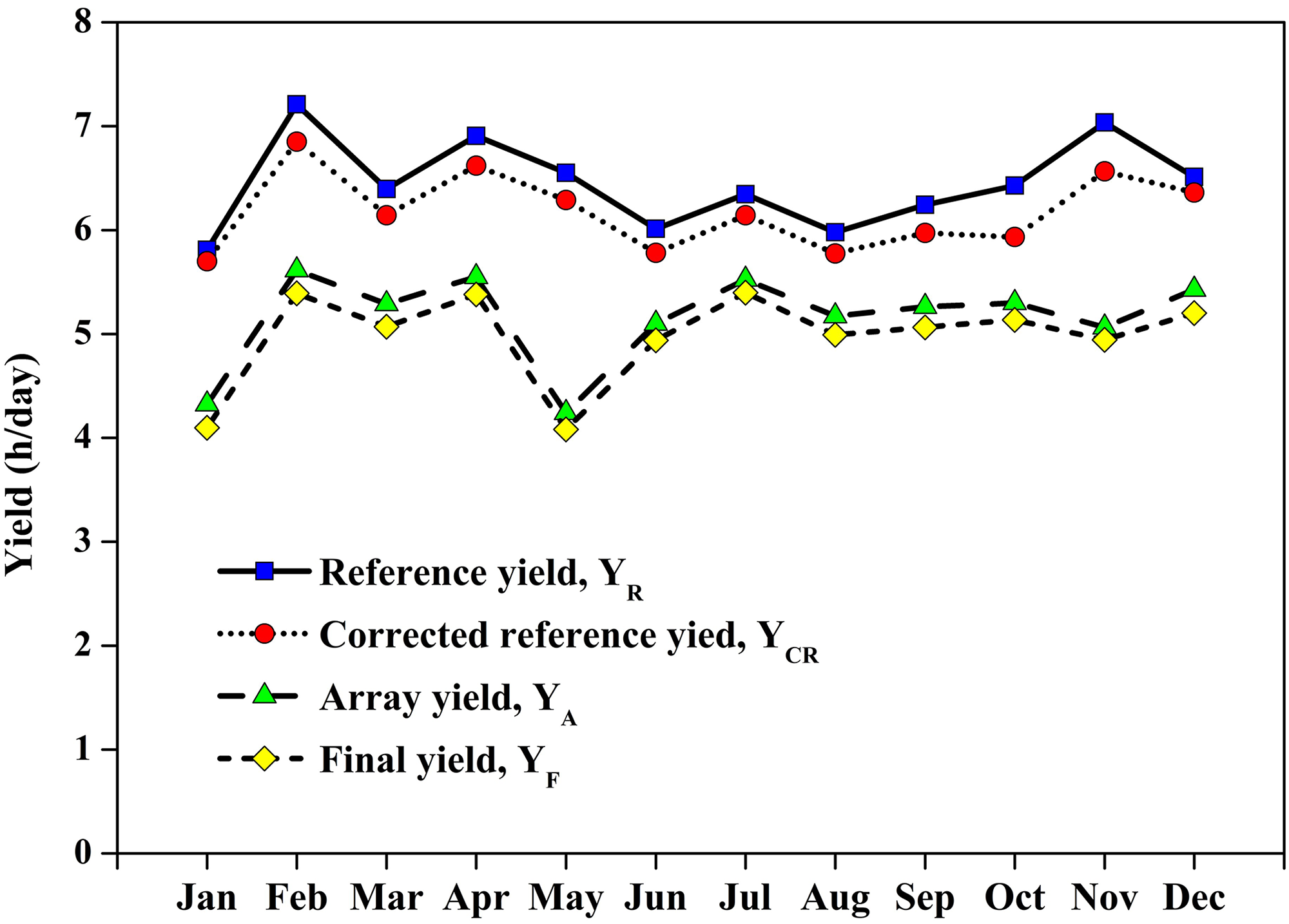
Daily monthly average of benchmark, corrected benchmark, array, and final GCPVS yields: Y_R (□), Y_CR (○), Y_A (Δ) & Y_F (◇).

Energy loss quantification

Capture losses from deassembly ranged from 0.81 h/day in August to 2.31 h/day in May, with an annual average of 1.30 h/day. System losses ranged from 0.12 h/day in November to 0.23 h/day in January, February, and December, with an annual mean of 0.18 h/day. Total losses show a range 1.52 h/day; that is, 2.47 h/day in May and 0.95 h/day in July, with an annual average of 1.48 h/day. As shown in Figure 5, May has the highest system loss, L_S, and total losses, L_O, with a maximum monthly mean temperature of 65.18°C and a monthly mean of 56.72°C. The month of May also presented the highest monthly mean temperature, with a variation from 25.2°C to 34.52°C, and an average of 31.54°C; a direct current energy, E_DC of 441.77 kWh/month, and a monthly mean solar insolation of 6.55 kWh/m². As can be seen, the largest loss is due to capture losses, L_C, that is, an annual average of 87.8%, while system losses, L_S, represent only 12.2% of the total losses, L_O.

Figure 5.

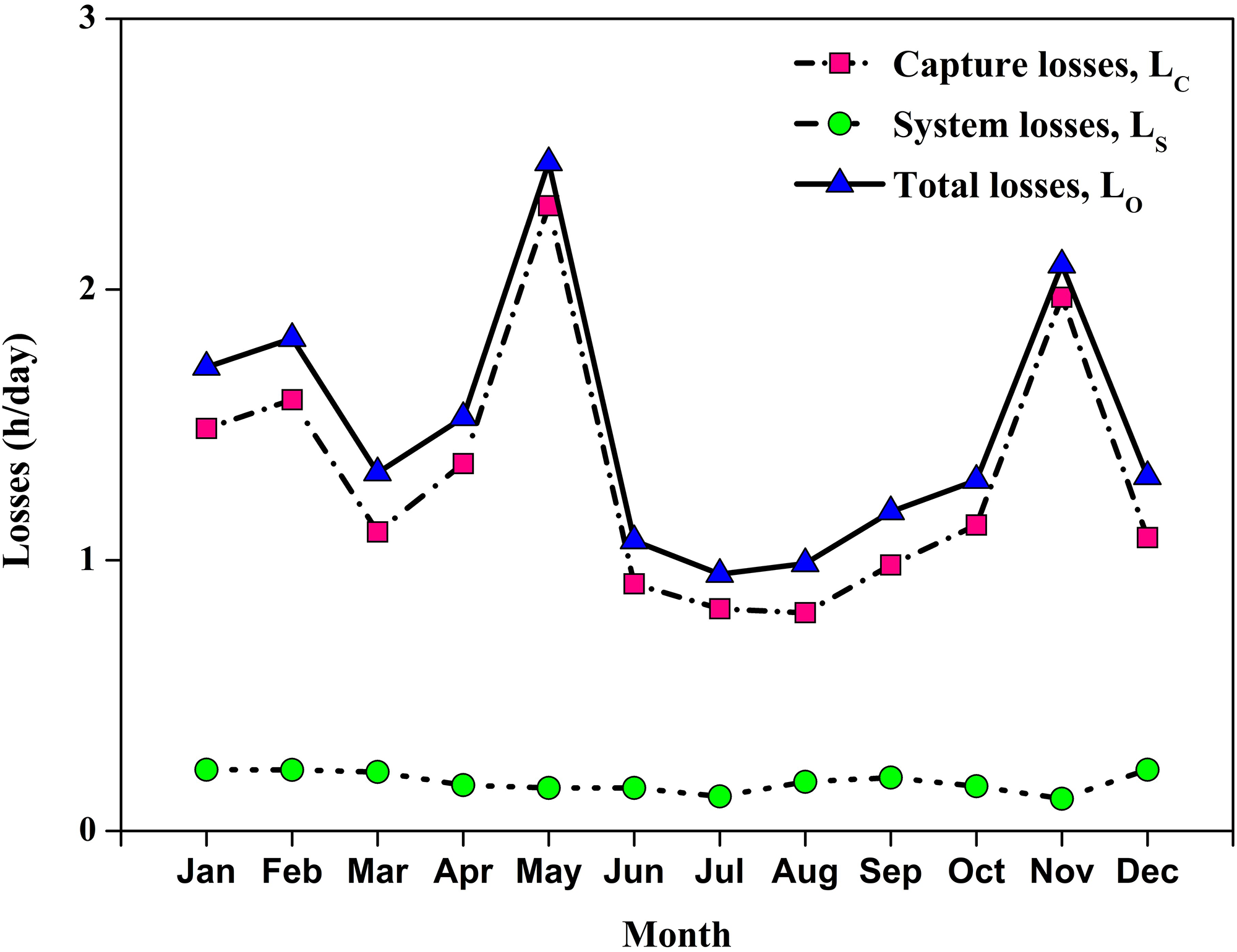
Monthly average daily catch, system, and overall losses: L_C (□), L_S (○), L_O (Δ).

System efficiency, PR, and capacity factor

Figure 6 illustrates the monthly average values of PV module efficiency (η_PVM), PVS efficiency (η_sys.), inverter efficiency (η_inv.), PR, and capacity factor (CF). PV module efficiency ranged from 10.30% in January to 12.42% in July; system efficiency ranged from 10.46% in May to 12.72% in July, and inverter efficiency ranged from 94.77% in January to 97.69% in July. The lowest values for system efficiency and PVM efficiency were obtained in May, compared to July, the month where the highest value was observed, with a difference of 25.63% for system efficiency, and 26.73% for PVM efficiency. The annual average efficiency of the system, modules, and inverter were 11.69%, 11.28%, and 96.46%, respectively. The PR varied from 62.32% in May to 85.05% in July, with an annual average of 77.22%, see Figure 7. Furthermore, the CF varied from 17.01% in May to 22.48% in July, with an annual average of 20.73%, while the PR presented a variation of 25.73%, while the CF varied about 24.36%.

Figure 6.

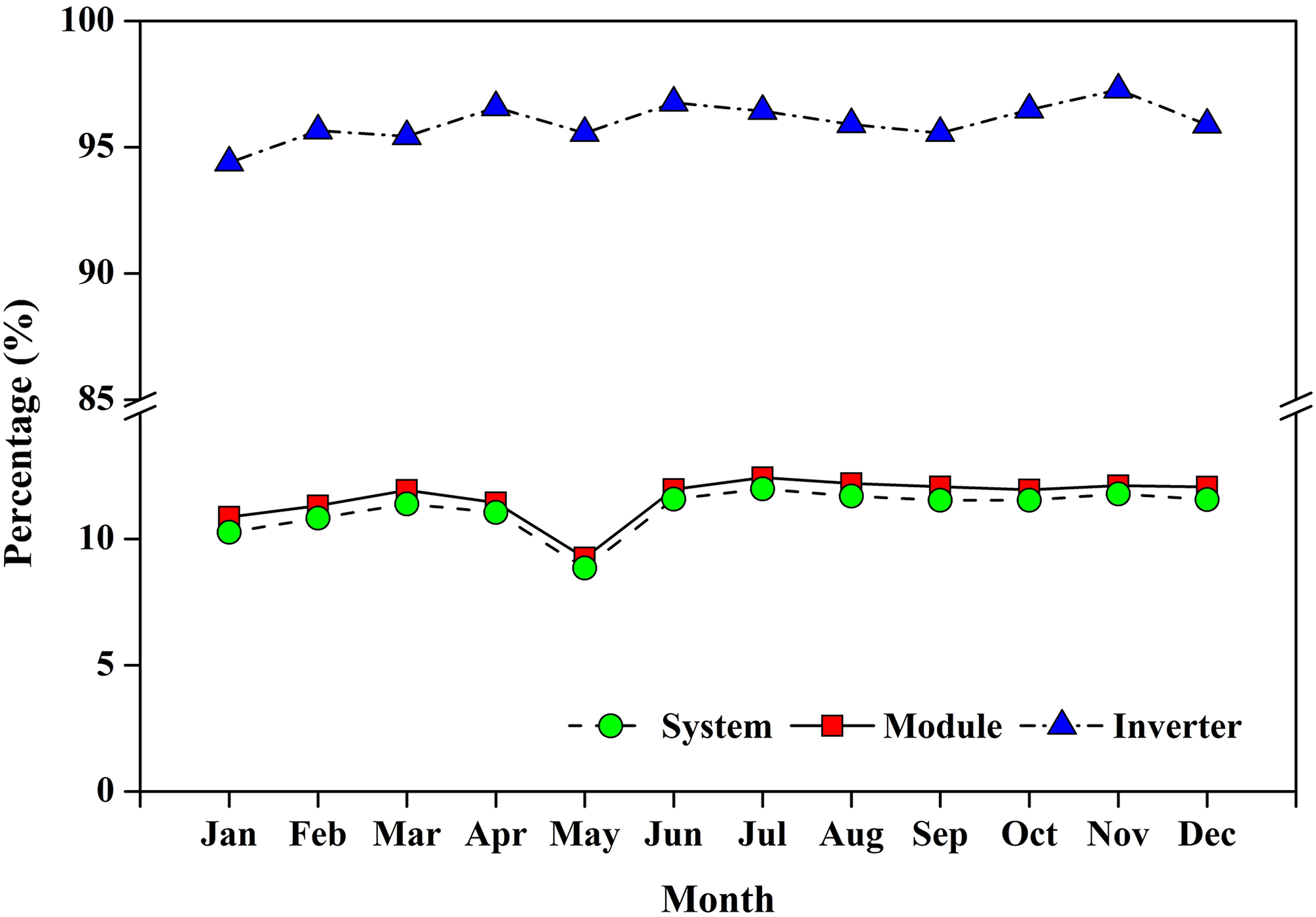
GCPVS monthly average efficiency (○), of the PV modules (□), and of the inverter (Δ).

Figure 7.

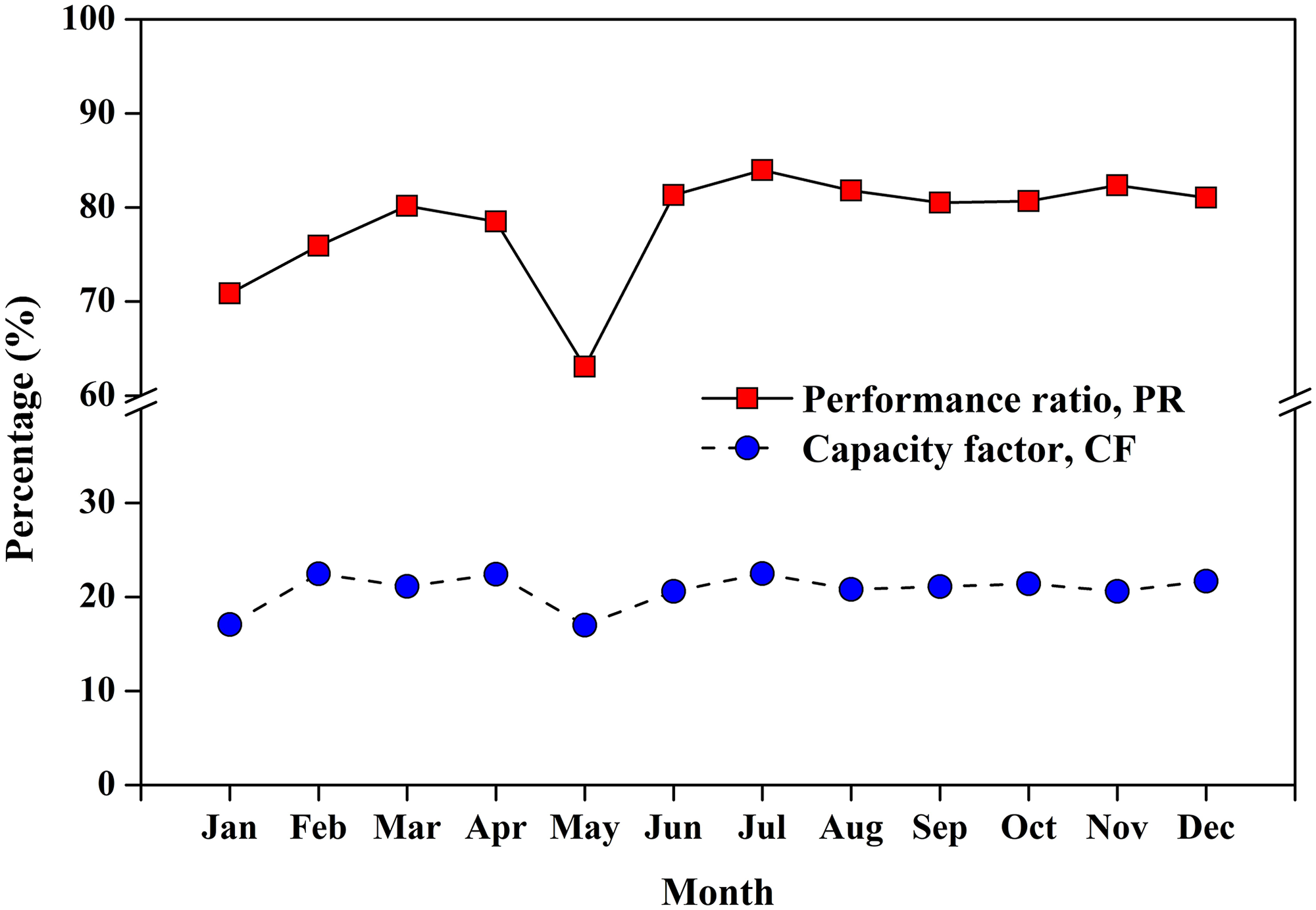
Monthly average of coefficient of performance, PR (□), and of the capacity factor, CF (○).

The efficiency of the PV modules for each month is shown in Figure 8, the mean and standard deviation of the efficiency: μ of 12.11%, and σ of 0.77%, respectively. The variability of the monthly average efficiency is minimal, which demonstrates the feasibility of implementing GCPVS for the studied local climatic conditions.

Figure 8.

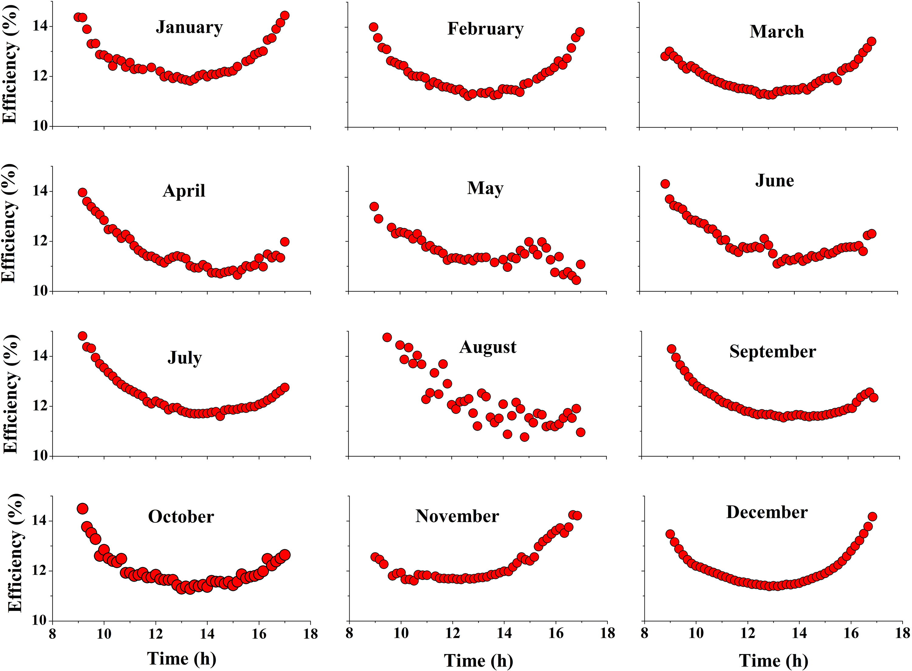
Monthly efficiency of the GCPVS through the year 2021.

Multivariate linear analysis

After the data processing, it was observed that all variables are influenced by the ambient temperature, in plane solar irradiance, wind speed, and module photovoltaics’ temperature. According to Hamou et al., the electrical efficiency of the PV module is a linear expression as shown in Equation (18).

η_{P V M} = η_{r e f .} [1 - β_{r e f .} (T_{m} - T_{r e f .})]

(18)

Equation (18) shows that PV system temperature is directly related to system efficiency. The magnitudes of the parameters η_ref. and β_ref. are temperature-dependent correction coefficients defined by the PVM manufacturer; the T_ref. is typically considered to be 25°C.

Climatological parameters and prediction models

According to experimental data, it was determined that the temperature variation of the photovoltaic module depends mainly on the ambient temperature and is less affected by wind speed (v). The result of the linear correlation given by Equation (19), which presented a determination coefficient of R²= 0.998.

η_{P V M} = a - b T_{m}

(19)

The efficiency of the PV system under actual operating conditions depends mainly on the PV module's temperature and the ambient temperature; the correlation of the PV system efficiency related to these parameters is shown in Equation (20), corresponding to a coefficient of determination of R²= 0.748. It is evident that the PV module temperature has an inverse relationship with the PVS efficiency. Likewise, the system efficiency also relies on the ambient temperature and wind speed, both parameters are correlated by Equation (21), which represents an MLR with a coefficient R²= 0.820. Furthermore, it is observed that the wind speed has an effect on the PVM temperature, improving the efficiency of the PV system, as it cools the overall surface of the system. In contrast, the ambient temperature has the opposite effect on the efficiency.

η_{s y s .1} = a - b T_{m} - c T_{a m b .}

(20)

η_{s y s .2} = a - b T_{m} - c T_{a m b .} - d G_{i} + e v

(21)

The E_DC generated power by the PVS is mainly related to the PV module temperature and solar irradiation intensity, its MLR is presented in Equation (22), with R²= 0.985. As can be seen from the mathematical fit, the intensity of solar irradiance has a positive impact, while the PVM temperature affects the power generation of the PV module, E_DC. Similarly, direct current energy was calculated considering the parameters of ambient temperature and wind speed, and R²= 0.990, see Equation (23). The parameters of the mathematically adjusted equations, the errors, and coefficients of determination are presented in Table 2.

E_{D C 1} = a - b T_{P V} + c G_{i}

(22)

E_{D C 2} = a + b T_{P V} + c G_{i} + d v - e T_{a m b .}

(23)

Table 2.

Summary of coefficient of the adjusted equations by MLR, error, and coefficient of determination.

Equation	Parameter	Error	R²
19	a = 0.162 b = 6.68 × 10⁻⁴	±7.13 × 10⁻⁵ ±1.30 × 10⁻⁶	0.998
20	a = 0.17 b = 9.19 × 10⁻⁴ c = 3.48 × 10⁻⁵	±1.4 × 10⁻³ ±3.24 × 10⁻⁵ ±7.47 × 10⁻⁵	0.748
21	a = 0.17 b = 1.54 × 10⁻⁵ c = 9.15 × 10⁻⁴ d = 2.69 e = 4.41	±1.5 × 10⁻³ ±6.71 × 10⁻⁵ ±8.66 × 10⁻⁵ ±1.74 × 10⁻⁶ ±1.51 × 10⁻⁴	0.820
22	a = 410.76 b = 4.01 c = 2.48	±23.90 ±0.73 ±0.023	0.985
23	a = 483.93 b = 49.73 c = 3.15 d = 14.9 e = 23.61	±19.43 ±0.97 ±0.023 ±2.17 ±1.25	0.990

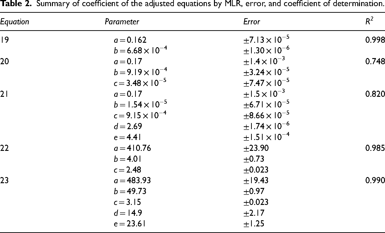
Both the efficiency of the PV modules, the system, and the direct current generation are influenced by the module's temperature and by the wind speed, which seems to be insufficient to cool the PV system, regardless the geographical location and the season of the year. The comparison between the experimental results and the prediction models obtained is shown in Figure 9. The uncertainty of the MLR fit of the efficiency of the PV module, system, and direct current generation is ±1.04%, ±0.57%, and ±35.38 kWh, respectively, which are lower compared with the reported by Adarmola and Vågnes (2015), Savvakis and Tsoutsos (2015) and Quansah et al., (2017).

Figure 9.

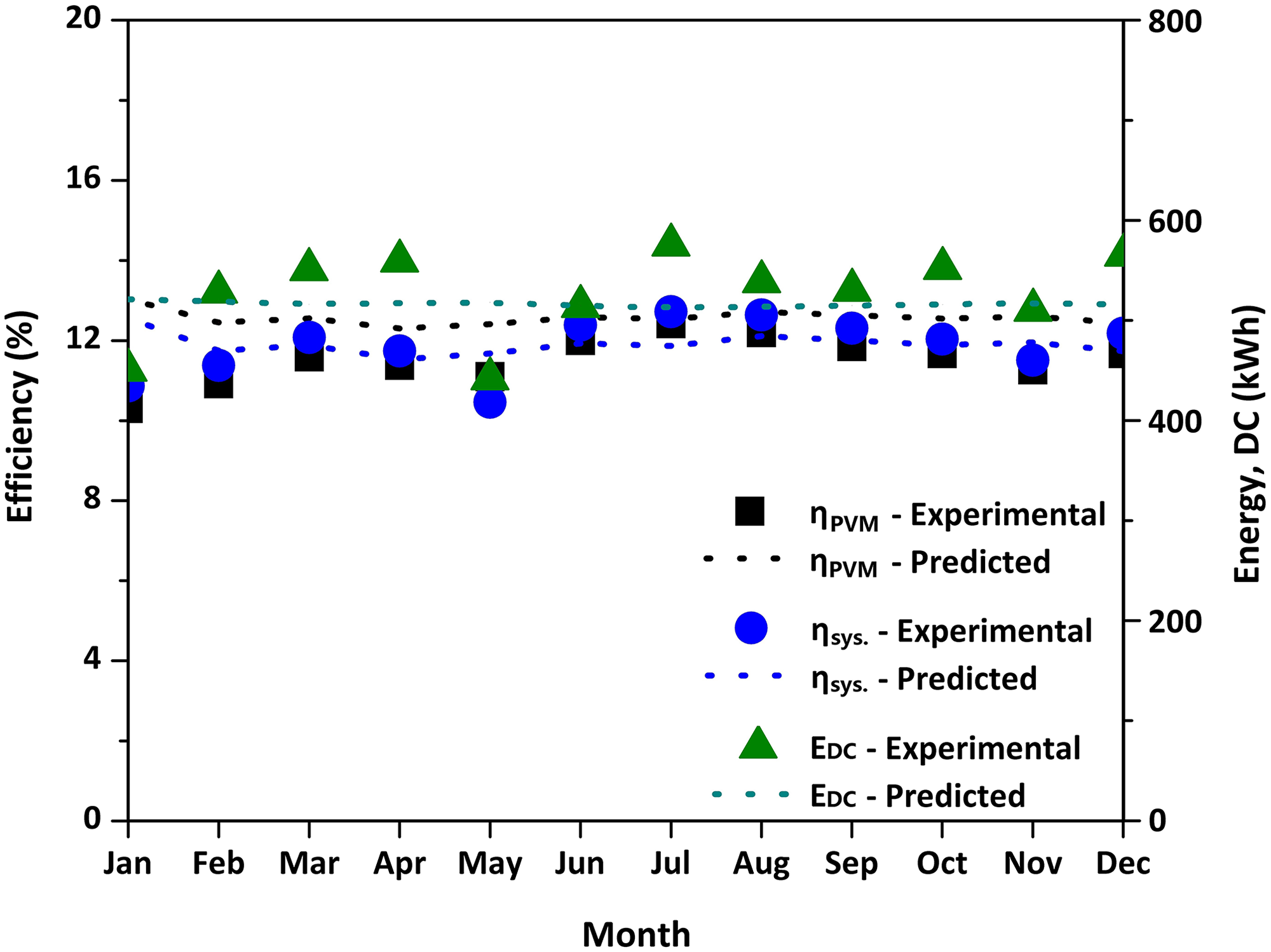
Comparison of the experimental results against MLR of PV module efficiency, system efficiency, and monthly direct current power.

Similarly, monthly DC energy generation was compared with the results obtained by simulation through a free software by The Concord Consortium, Energy3D (Xie et al., 2018). Figure 10 shows the in situ PVS; details of the Energy3D interface, and the Energy3D initial conditions used in simulation, which were taken from Table 1. The comparison between the experimental results and the simulation exhibits an average absolute error of ±2.33 kWh, in the annual generation; as shown in Figure 11.

Figure 10.

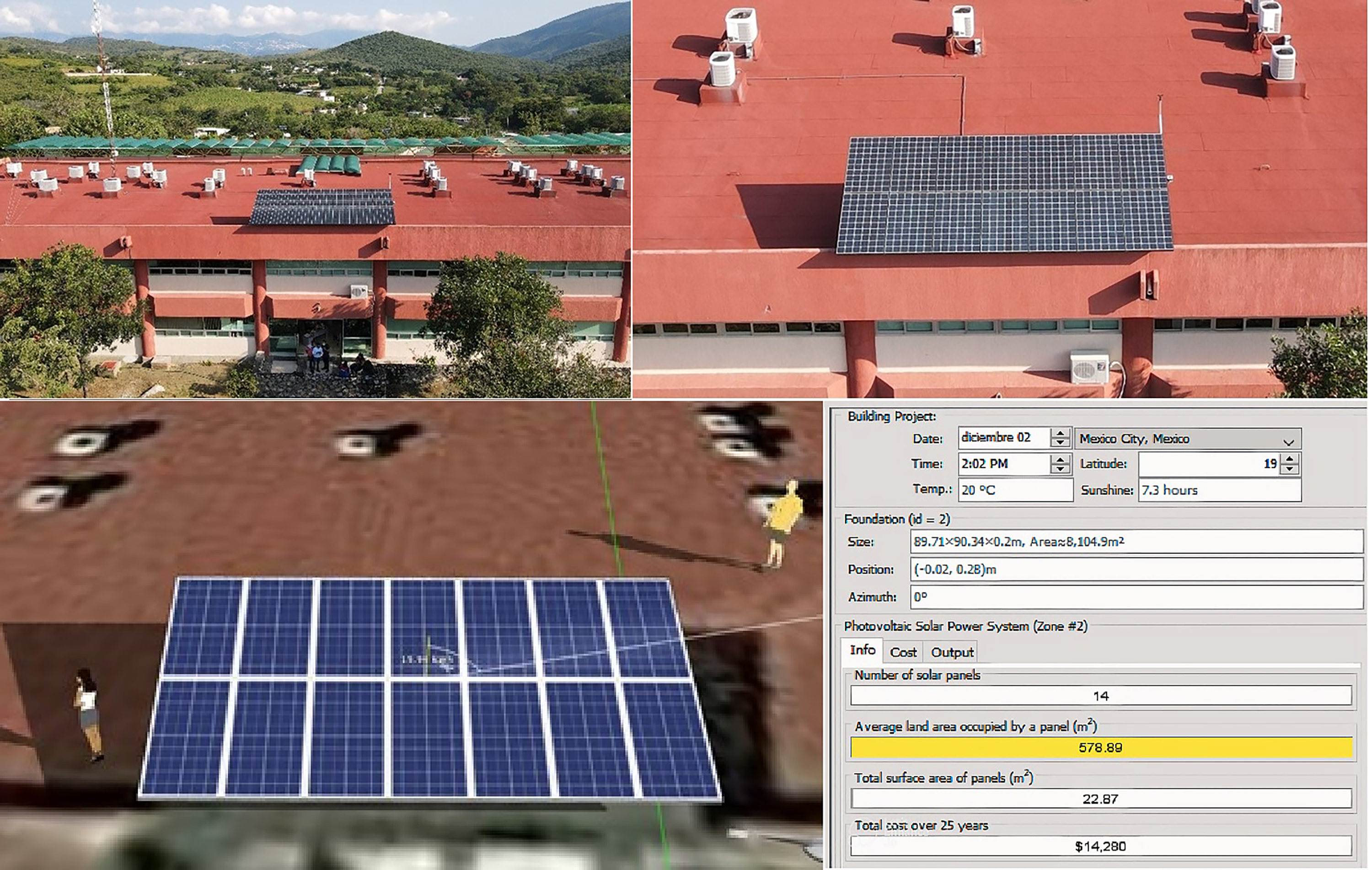
Photograph of actual GCPVS taken with a drone (top, left); close-up of drone photo, (top, right); isometric view from the Energy3D program including the PVS (bottom-left); and initial conditions used in simulation (bottom, right).

Figure 11.

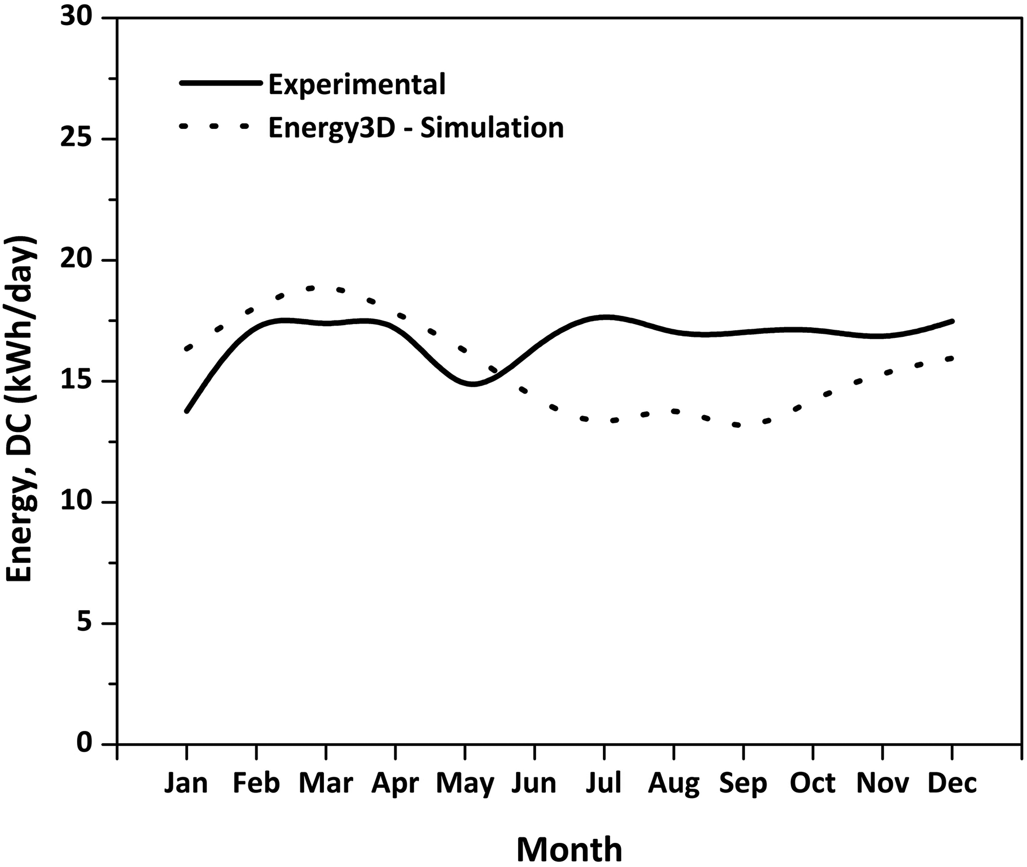
Comparison of the experimental results against those obtained by Energy3D simulation free software, of the monthly direct current generated energy.

Conclusions

The existence of predictive models of the performance of a GCPVS using in situ data in the region of interest is essential to assessing preinstallation and investment performance, to ensure, with a certain degree of uncertainty, the correct operation of GCPVS, which can be implemented at another similar geographic area and climate around the world. The operating temperature of the PV module plays an important role in the energy conversion process. The annual average reference yield (Y_R), corrected reference yield (Y_CR), array yield (Y_A), and final yield (Y_F) were 6.45 h/day, 6.18 h/day, 5.16 h/day, and 4.97 h/day, respectively. The total amount of CO₂ not released to the environment was 4714.92 kg/year. The average annual overall capacity factor and performance coefficients were 20.73% and 77.22%, correspondingly. Concerning to the different types of losses: L_C, L_S, and L_O were 0.82 h/day, 0.13 h/day, and 0.95 h/day; while the PR and capacity factor were 85.05% and 22.48%, respectively. This indicates that climatic conditions significantly affect the performance of the GCPVS. In this study, models for predicting photovoltaic module efficiency, system efficiency, and direct current generation were developed, applied, and compared againts simulation. Multiple variable regression analyses showed that wind speed has a positive effect on the PVS performance, and its MLR has a correlation coefficient R² of 0.990. The uncertainty of the MLR fit for PV module efficiency, system efficiency, and direct current generation is ±1.04%, ±0.57%, and ±35.38 kWh, individually. Finally, the monthly energy generation was compared by simulation through Energy3D free software, showing an absolute error of ±2.33 kWh. The obtained results can serve as a methodological tool to predict and simulate the efficiency and direct current energy generation in GCPVS at different regions.

Footnotes

Acknowledgements

The authors wish to thank research professor David Becerra García for his collaboration in the review of the state of the art; they also thank engineer Óscar Omar Zaragoza Landa for the photograph taken with a drone. Also, the authors want to specially thanks to engineer Manuel Mena Vargas for the English grammar & spelling review.

Author contribution

All authors contributed to the study conception and design. Material preparation, data collection and analysis were performed by MA Rivera-Martínez and J.A. Alanís-Navarro. The first draft of the manuscript was written by J.A. Alanís-Navarro and MA García-López. Finally, M. Fuentes-Pérez and J.E. Lavín-Delgado detected and made the corrections to the manuscript. All authors read carefully and approve the final manuscript.

Declaration of conflicting interests

The authors declared no potential conflicts of interest with respect to the research, authorship, and/or publication of this article.

Funding

The authors received no financial support for the research, authorship, and/or publication of this article.

Ethical approval

This study does not contain any studies with human or animal subjects performed by any of the authors.

ORCID iD

José Andrés Alanís-Navarro

Data availability

Additional data and material to those reported in the experimental section can be shared upon request.

List of symbols

References

Adaramola

Vågnes

EET

(2015) Preliminary assessment of a small-scale rooftop PV-grid tied in Norwegian climatic conditions. Energy Conversion and Management 90: 458–465.

Akhter

Mekhilef

Mokhlis

, et al. (2020) Performance assessment of three grid-connected photovoltaic systems with combined capacity of 6.575 kWp in Malaysia. Journal of Cleaner Production 277: 123242.

Akpolat

Dursun

Kuzucuoğlu

, et al. (2019) Performance analysis of a grid-connected rooftop solar photovoltaic system. Electronics 8(8): 905.

Al-Badi

(2018) Measured performance evaluation of a 1.4 kW grid connected desert type PV in Oman. Energy for Sustainable Development 47: 107–113.

Alshare

Tashtoush

Altarazi

, et al. (2020) Energy and economic analysis of a 5 MW photovoltaic system in northern Jordan. Case Studies in Thermal Engineering 21: 100722.

de Lima

Ferreira

de Lima Morais

FHB

(2017) Performance analysis of a grid connected photovoltaic system in northeastern Brazil. Energy for Sustainable Development 37: 79–85.

Dondariya

Porwal

Awasthi

, et al. (2018) Performance simulation of grid-connected rooftop solar PV system for small households: A case study of Ujjain, India. Energy Reports 4: 546–553.

Enerdata (2021) World Energy & Climate Statistics-Yearbook 2022. Total energy generation. Available at: https://yearbook.enerdata.net/total-energy/world-energy-production.html (accessed on 20 July 2020).

Gielen

Boshell

Saygin

, et al. (2019) The role of renewable energy in the global energy transformation. Energy Strategy Reviews 24: 38–50.

10.

Pinheiro

HHC

da Silva

Branco

DAC

, et al. (2020) Photovoltaic solar systems in multi-headquarter institutions: A technical implementation in northeastern Brazil. Energies 13(10): 2659.

11.

Quansah

Adaramola

Appiah

, et al. (2017) Performance analysis of different grid-connected solar photovoltaic (PV) system technologies with combined capacity of 20 kW located in humid tropical climate. International Journal of Hydrogen Energy 42(7): 4626–4635.

12.

Savvakis

Tsoutsos

(2015) Performance assessment of a thin film photovoltaic system under actual Mediterranean climate conditions in the island of crete. Energy 90: 1435–1455.

13.

SENER (2017) Reporte de Avance de Energías Limpias Primer Semestre 2018. Ciudad de México. SENER. Available at: https://www.gob.mx/sener/documentos/informe-sobre-la-participacion-de-las-energias-renovables-en-la-generacion-de-electricidad-en-México-al-30-de-junio (accessed 22 July 2020) (in Spanish).

14.

SENER (2018) Balance Nacional de Energía 2018. Ciudad de México: SENER. Available at https://www.gob.mx/cms/uploads/attachment/file/528054/Balance_Nacional_de_Energ_a_2018.pdf (accessed 20 July 2020) (in Spanish).

15.

SENER (2020) Balance nacional de energía 2020. Ciudad de México. SENER. Available at https://www.gob.mx/cms/uploads/attachment/file/707654/BALANCE_NACIONAL_ENERGIA_0403.pdf (accessed 20 July 2020) (in Spanish).

16.

Tahri

Oozeki

(2018) Performance evaluation of grid-connected photovoltaic systems based on two photovoltaic module technologies under tropical climate conditions. Energy Conversion of Management 165: 244–252.

17.

Thotakura

Kondamudi

Xavier

, et al. (2020) Operational performance of megawatt-scale grid integrated rooftop solar PV system in tropical wet and dry climates of India. Case Studies in Thermal Engineering 18: 100602.

18.

Xie

Schimpf

Chao

, et al. (2018) Learning and teaching engineering design through modeling and simulation on a CAD platform. Computer Applications in Engineering Education 26(4): 824–840.

Theoretic and experimental performance of a grid-connected photovoltaic system: Multiple prediction model of efficiency and annual energy generation