Sage Journals: Discover world-class research

Abstract

The advancement of horizontal drilling and hydraulic fracturing technologies has led to an increased significance of shale gas as a vital energy source. In the realm of oilfield development decisions, production forecast analysis stands as an essential aspect. Despite numerical simulation being a prevalent method for production prediction, its time-consuming nature is ill-suited for expeditious decision-making in oilfield development. Consequently, we present a data-driven model, ASGA-XGBoost, designed for rapid and precise forecasting of shale gas production from horizontally fractured wells. The central premise of ASGA-XGBoost entails the implementation of ASGA to optimize the hyperparameters of the XGBoost model, thereby enhancing its prediction performance. To assess the feasibility of the ASGA-XGBoost model, we employed a dataset comprising 250 samples, acquired by simulating shale gas multistage fractured horizontal well development through the use of CMG commercial numerical simulation software. Furthermore, XGBoost, GA-XGBoost, and ASGA-XGBoost models were trained using the data from the training set and employed to predict the 30-day cumulative gas production utilizing the data from the testing set. The outcomes demonstrate that the ASGA-XGBoost model yields the lowest mean absolute error and offers optimal performance in predicting the 30-day cumulative gas production. Additionally, the mean absolute error of the unoptimized XGBoost model is markedly greater than that of the optimized XGBoost model, indicating that the latter, refined through the application of intelligent optimization algorithms, exhibits superior performance. The insights gleaned from this investigation have the potential to inform the development of strategic plans for shale gas oilfields, ultimately promoting the cost-effective exploitation of this energy resource.

Keywords

Shale gas fracturing horizontal well ASGA XGBoost production prediction

Introduction

Natural gas has emerged as a critical component of the global energy framework due to its high fuel value and low pollution (Barnes and Bosworth, 2015; Najibi et al., 2009; Reymond, 2007). Nevertheless, the world's burgeoning economy has rendered conventional gas reserves insufficient to satisfy societal demands (Abdul et al., 2021; Bhuiyan et al., 2022; Li et al., 2021). Consequently, an increasing number of studies are focusing on the exploration and production of unconventional gas resources (Song et al., 2017; Umbach, 2013; Wang and Lin, 2014). Shale gas, an unconventional gas with substantial global reserves (Guo et al., 2017), was once deemed unfeasible to extract due to its adsorption properties and super-low permeability and porosity (Zhang et al., 2015). Nevertheless, advancements in horizontal well fracturing technology have rendered shale gas extraction achievable (Liang et al., 2012; Lin et al., 2018; Wang et al., 2016). The horizontal wellbore facilitates the positioning of hydraulic fractures in various orientations, significantly enhancing permeability in the wellbore's vicinity and, consequently, bolstering gas production.

Predicting production is a critical aspect of oilfield development decision-making. There exist two primary types of production prediction models: Those driven by physical principles (Hu et al., 2016) and those driven by data (Liu et al., 2014). Physical-driven models can be further divided into analytical models (Cossio et al., 2013) and numerical simulation models (Paul et al., 2019). Analytical models aim to derive solutions based on seepage theory, as demonstrated by Lin et al. (2022), who developed a productivity prediction model for shale gas fractured horizontal wells, taking into account factors such as the fracture network's complexity, stress sensitivity effects, adsorption, and desorption. While analytical models offer rapid computation, their accuracy in predicting production from horizontal wells under complex conditions is limited due to the numerous assumptions involved. In contrast, numerical simulation models have the capacity to simulate intricate seepage situations and estimate production based on a wide range of reservoir data, encompassing geological, and drilling data. Theoretically, the accuracy of these models improves as more comprehensive data is considered. Yuan et al. (2018) established a shale gas discrete fracture network model based on an unstructured vertical bisection grid to predict the production of the shale gas fracturing horizontal well. While numerical simulation models often outperform their analytical counterparts in production prediction, their computational demand can be overwhelming for practical implementation.

In recent years, machine learning has been widely applied in the energy field, such as investment analysis of green energy projects (Hasan et al., 2022), levelized cost analysis (Li et al., 2022), analysis of financial development and open innovation (Alexey et al., 2023), oil production prediction (Cheng and Yang, 2021), and so on. Data-driven models, built by machine learning algorithms, could get the functional relationship between the production and its influencing parameters thanks to a training process based on available data (Mirzaei-Paiaman and Salavati, 2012). In general, data-driven models could be the substitute for physics-driven models. Compared with physics-driven models, data-driven models have no presumed functional relationship, and the functional relationships are obtained from the training data (Kulgaa et al., 2017). Chen et al. (2022) established a productivity prediction model of shale gas horizontal wells by the long short-term memory (LSTM) network. Wang et al. (2022) predicted the production of the shale gas horizontal well by building a deep learning network. Data-driven models offer high prediction accuracy and fast calculation speed, although ensuring optimal hyperparameters for the utilized machine learning algorithm is crucial to their accuracy.

Intelligent optimization algorithms, such as genetic algorithms (GAs) (Irani et al., 2011) and particle swarm optimization (PSO) (Nasimi et al., 2012), offer feasible approaches to hyperparameter optimization. Irani et al. (2011) established a neural network model coupled with GA to predict permeability. David et al. (2022) predicted the optimal rate of penetration by the multilayer perceptron model optimized by the GA. Li et al. (2022) proposed a PSO-CNN-LSTM model to solve the time-series prediction problems. Massive researches clearly indicate that intelligent optimization algorithms can drastically improve the performance of data-driven models in production prediction. Nonetheless, these algorithms vary in their adaptability to specific data-driven models, requiring further research to explore their suitability for different scenarios.

In this study, a prediction model named ASGA-XGBoost was proposed to predict the 30-day cumulative gas production of the shale gas horizontal fracturing well. In the process, ASGA, an improved GA, was used to search for the optimal hyperparameter combination of the XGBoost model. Compared with the GA-XGBoost model, ASGA-XGBoost has better performance in predicting the 30-day cumulative gas production of the shale gas horizontal fracturing well. The prediction results can provide help for the formulation of a shale gas oilfield development plan, resulting in the economic and effective development of shale gas.

Methodology

XGBoost algorithm

Extreme gradient boosting (XGBoost) is a prominent ensemble algorithm that integrates a vast array of weak learners to generate a strong learner (Chen and Guestrin, 2016). Typically, XGBoost relies on the classification and regression tree (CART) as its fundamental learner, which is well-suited to solve classification and regression problems. Owing to its superior performance, XGBoost has been extensively implemented in the petroleum industry, including sweet spot searching (Tang et al., 2021), dynamometer-card classification (Chris, 2020), and water absorption prediction (Liu et al., 2020).

XGBoost is renowned for its exceptional computation speed and remarkable prediction accuracy. As a supervised machine learning method, XGBoost leverages the input and output parameters of the dataset for modeling purposes. The algorithm functions through a process of incrementally integrating multiple base learners to consistently improve the residual reduction. As illustrated in Figure 1, each base learner is iteratively added to the ensemble, and the output prediction result is determined as mentioned below:

{\hat{y}}_{i}^{(t)} = {\hat{y}}_{i}^{(t - 1)} + f_{t} (x)

(1)where

{\hat{y}}_{i}^{(t)}

is the predicted value of the ith sample after iteration t,

f_{t} (x)

denotes the calculated value of the tth base learner. And the objective function is shown as mentioned below:

Obj = \sum_{i = 1}^{n} l (y_{i} - {\hat{y}}_{i}^{(t)}) + \sum_{i = 1}^{t} Ω (f_{i})

(2)where

y_{i}

denotes the actual value, and l represents the loss function.

Ω

indicates the regularization term, which can adjust the model complication and reduce overfitting.

Figure 1.

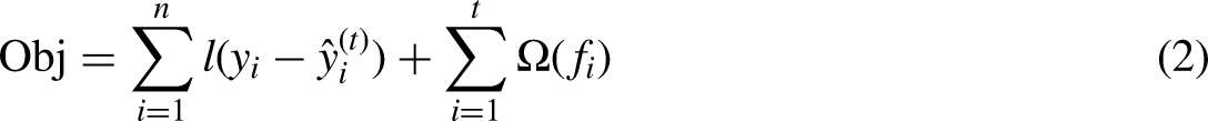
The workflow of the XGBoost algorithm. In the process, each tree is built to fit the residual of the previous tree. The final prediction result is obtained by synthesizing the calculation results of all trees.

XGBoost has ten hyperparameters, including booster, n_estimators, max_depth, min_child_weight, eta, gamma, subsample, colsample_bytree, reg_alpha, and reg_lambda. Booster determines the type of base learner, usually a decision tree, and n_estimators is the number of base learners. For tree booster, max_depth denotes the maximum depth and min_child_weight is the minimum sum of leaf node sample weights. Eta represents the learning rate, which can be decreased to reduce overfitting. gamma indicates the minimum loss function drop for node splitting. subsample decides the proportion of random samples for each base learner. colsample_bytree is the subsample ratio of columns when constructing each tree. reg_alpha represents the L1 regularization term and reg_lambda denotes the L2 regularization term. These ten hyperparameters are key determinants for optimizing the prediction accuracy of XGBoost model. Hence, obtaining optimal hyperparameters is crucial for the XGBoost model's optimal functionality.

ASGA-XGBoost model

In this study, a modified adaptive GA based on the Spearman correlative coefficient (ASGA) was proposed to get the optimal hyperparameters. GA, proposed by John Holland first, is a method for searching for the optimal solution by simulating the natural evolution process (John, 1992). Over the past few decades, GA has extensively found applications in multiple optimization problems (Karen, 2005; Wathiq and Maytham, 2011; Souza et al., 2018). However, GA frequently necessitates numerous iterations to arrive at the most fitting solution, leading to prolonged optimization times. In other words, GA optimization accuracy is typically challenging to sustain within a certain number of iterations. Zhou and Ran (2023) proposed a modified GA based on the Spearman correlative coefficient (SGA) to improve the optimization speed and accuracy. Compared to GA, SGA modifies the crossover and mutation rates’ determination methods. Generally, in GA, each gene has the same crossover and mutation rates, which can prolong the search for the optimal solution. The purpose of SGA is to approach the optimal solution quickly by adjusting the crossover and mutation rates of the genes.

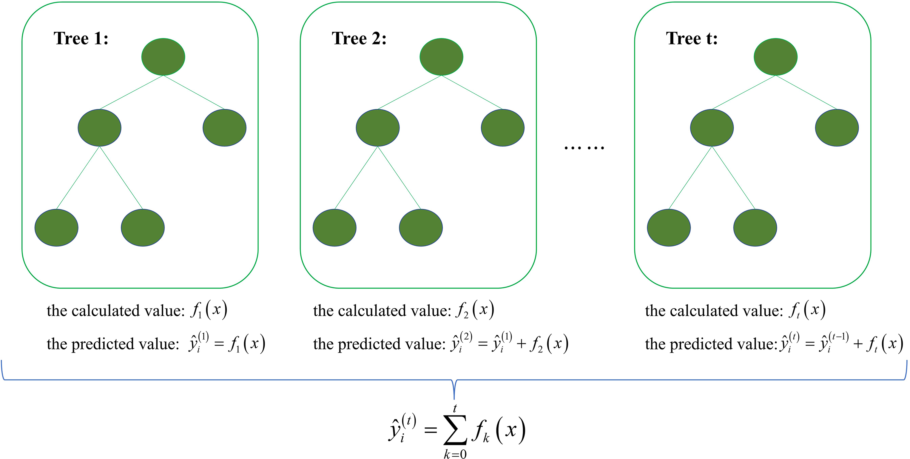
However, SGA necessitates a dataset containing optimized hyperparameters and the optimization objective to determine Spearman correlation coefficients between parameters and objectives, subsequently determining the mutation and crossover rates. In this study, the ten hyperparameters of the XGBoost model constitute the optimized parameters, and the validation error of the XGBoost model becomes the optimization objective. Nonetheless, the absence of datasets containing hyperparameters and validation errors precludes the direct application of SGA to optimize XGBoost's hyperparameters. To address this, a modified SGA, referred to as ASGA, was introduced. ASGA integrates a dataset creation process to calculate Spearman correlation coefficients. Specifically, the new individuals and their corresponding validation errors in each iteration process are added to the dataset to increase the number of data samples. Accordingly, each iteration process necessitates recalculating the Spearman correlation coefficient, and the crossover and mutation rates differ for each step. The incorporation of ASGA helps XGBoost models identify optimal hyperparameters and enhance performance in production prediction. As depicted in Figure 2, the workflow of ASGA-XGBoost is as follows:

Figure 2.

The workflow of the ASGA-XGBoost model. There are 7 steps to achieve the ASGA-XGBoost algorithm. Its main idea is getting the best hyperparameters of the XGBoost model through a large number of iterative calculations.

Step 1—Population Initialization. The population consists of a certain number of individuals, also called chromosomes, and each chromosome is composed of some genes. In this study, each gene denotes a hyperparameter of the XGBoost model. In this process, n individuals are obtained by randomly generating the hyperparameters within limits.

Step 2—Fitness Calculation. Fitness serves as a crucial criterion for selecting desirable individuals for breeding in the subsequent generation. In this study, the fitness is calculated by the validation error of the XGBoost model, where smaller validation errors indicate higher fitness.

Step 3—Selection Operation. The purpose of the selection operation is to inherit the excellent individuals to the next generation. Roulette wheel selection is the most common way to select individuals from the population as parents. In this process, each individual in the population has a probability of being selected, which is associated with fitness. In general, individuals with higher fitness have a greater probability of selection. Moreover, the operation of roulette wheel selection needs to be repeated n times to get n pairs of individuals as parents, which are used to get the next generation via crossover and mutation operation.

Step 4—Calculation of the Crossover and Mutation Rates. Firstly, a dataset including the hyperparameters and training error of the XGBoost model should be established. In the optimization process, the new population obtained in each iteration needs to be put in the dataset.

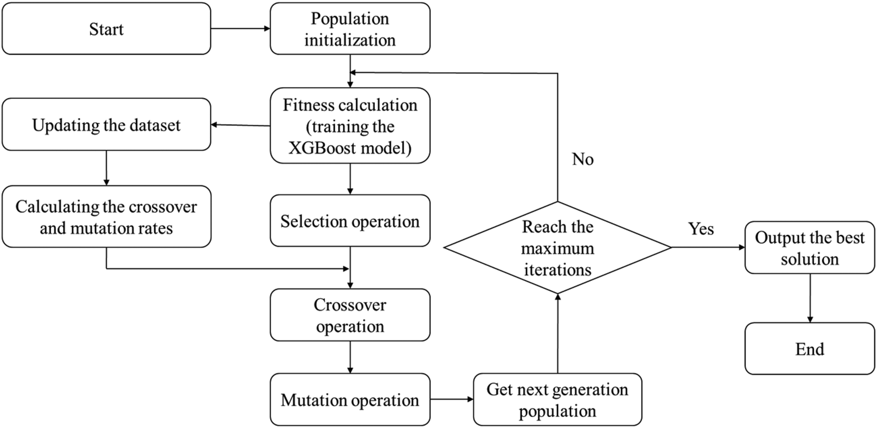
Secondly, the Spearman correlative coefficients between the hyperparameters and the validation error could be calculated. Correlation coefficients, such as Pearson, Kendall, and Spearman, are primarily used to represent the correlation between two parameters. The Pearson correlation coefficient works well only in describing the linear relationship of two continuous variables with a positive distribution. Nevertheless, the relationships between the hyperparameters and the validation error might be nonlinear. Moreover, the Kendall correlation coefficient is usually applied to the rank variables while most hyperparameters are continuous variables. Compared with the two methods, the Spearman correlation coefficient has no requirement for data distribution and variables. Furthermore, it also can indicate correlations between two variables that are linear or even partially non-linear. Therefore, the Spearman correlation coefficient is selected to calculate the correlative coefficients of the hyperparameters and the validation error. The Spearman correlation coefficient can be calculated by:

ρ_{i} = \frac{\sum_{j = 1}^{n} (d_{i j} - {\bar{d}}_{i}) (s_{j} - \bar{s})}{\sqrt{\sum_{j = 1}^{n} {(d_{i j} - {\bar{d}}_{i})}^{2} \sum_{j = 1}^{n} {(s_{j} - \bar{s})}^{2}}}

(3)where

ρ_{i}

is the Spearman correlative coefficient of the ith hyperparameter, and n represents the number of samples.

d_{i j}

denotes the rank of the jth sample sorted according to the jth hyperparameter, and

{\bar{d}}_{i}

is the mean rank of the samples sorted according to the ith hyperparameter.

s_{j}

denotes the rank of the jth sample sorted according to the validation error, and

\bar{s}

is the mean rank of the samples sorted according to the validation error. Generally, a higher absolute value of the Spearman correlative coefficient indicates a stronger correlation between the hyperparameter and validation error. However, do note that a smaller correlative coefficient does not necessarily imply a weak correlation, meaning this statistic can only represent the hyperparameters’ importance to the validation error up to a certain degree. Even so, the correlative coefficient remains a critical performance indicator for assessing correlation.

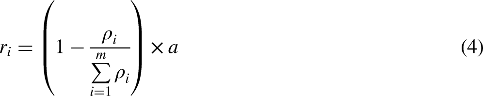
Thirdly, the crossover and mutation rates could be gotten by the calculated Spearman correlative coefficients. In this study, the gene with a high Spearman correlative coefficient has low crossover and mutation rates so the excellent gene has a greater probability of retention. To achieve this purpose, the crossover and mutation rates could be calculated by:

r_{i} = (1 - \frac{ρ_{i}}{\sum_{i = 1}^{m} ρ_{i}}) \times a

(4)where

r_{i}

denotes the crossover and mutation rates of the ith gene, and m is the number of hyperparameters. a is the control factor, which could limit the crossover and mutation rates. In general, crossover and mutation operations have different values of a.

Step 5—Crossover Operation. The process of crossover operation is to cross one or more genes on two individuals to get a new individual. Based on the calculation crossover rates of Step 4, each gene has a probability to decide whether to be crossed or not. In this step, n new individuals could be obtained by crossing the n pair of individuals selected thanks to the selection operation.

Step 6—Mutation Operation. Mutation operation is mainly used for the n new individuals generated by crossover operation. Its purpose is to get a new population by randomly changing the genes of the new individuals. Similarly, each gene has a probability to decide whether to be changed, which is calculated in Step 4. After mutation operation, a population with n new individual could be gotten.

Step 7—Output the Optimal Solution. Repeat Steps 2–6 until reaching the maximum iterations. Then, the individual with the greatest fitness is outputted as the optimal solution.

Application

Data description

To assess the applicability of this approach, the CMG commercial numerical simulation software was employed to simulate multistage fracturing horizontal well development for shale gas extraction. The resultant data encompassed geological, fracturing, and production parameters. Specifically, six parameters, including porosity, permeability, the number of fracturing sections, the length of the horizontal well, fracture width, and fracture half-length, served as the inputs for the XGBoost model, while the 30-day cumulative gas production constituted the output.

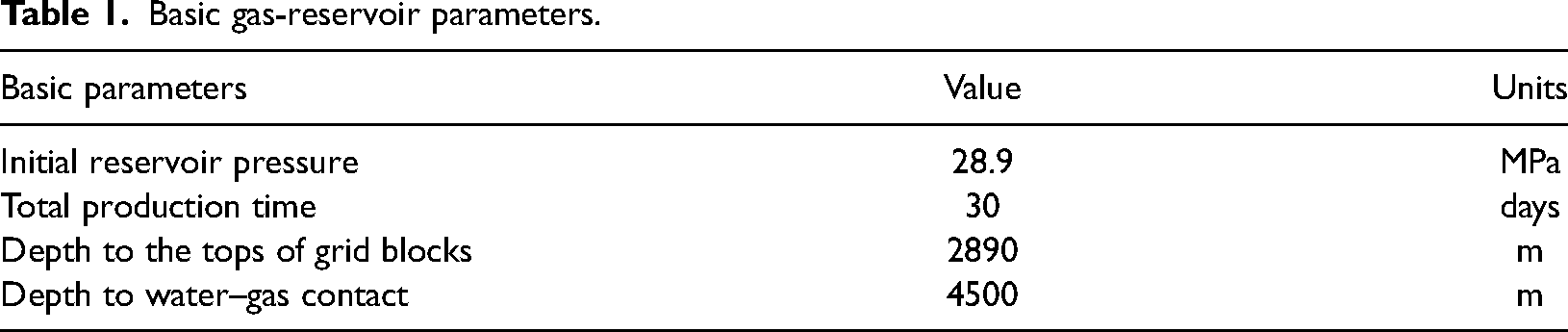
Figure 3 displays the shale gas reservoir, which was established using the CMG commercial numerical simulation software, possessing dimensions of 3000 × 3000 × 100 m. The grid's dimensions measure 200 × 200 × 10, with a spacing of 15 m in the I and J directions and 10 m in the K direction, as indicated in Table 1. The shale gas horizontal well is located in the fifth layer, and perforation produces vertical fractures.

Figure 3.

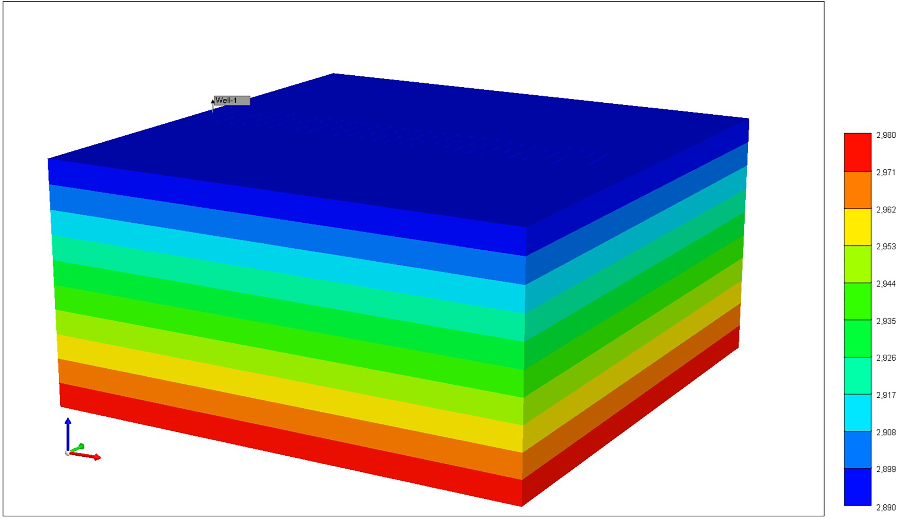
Numerical simulation of the shale gas fracturing horizontal well. There are 10 layers in the reservoir and the horizontal well is located in the fifth layer.

Table 1.

Basic gas-reservoir parameters.

Basic parameters	Value	Units
Initial reservoir pressure	28.9	MPa
Total production time	30	days
Depth to the tops of grid blocks	2890	m
Depth to water–gas contact	4500	m

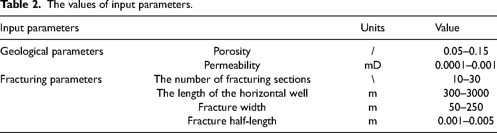
To get the dataset for the XGBoost model, three steps need to be done. Firstly, based on the bounds of the input parameters shown in Table 2, the geological and fracturing parameters were generated randomly by a computer program. Secondly, the cumulative gas production of the horizontal well could be calculated by inputting the geological and fracturing parameters into the established CMG numerical model. Thirdly, the dataset could be gotten by repeating the two steps. In this study, a dataset with 250 groups of samples was obtained. Figure 4 gives the distributions between input parameters and output parameter.

Table 2.

The values of input parameters.

Input parameters		Units	Value
Geological parameters	Porosity	/	0.05–0.15
Geological parameters	Permeability	mD	0.0001–0.001
Fracturing parameters	The number of fracturing sections	\	10–30
	The length of the horizontal well	m	300–3000
	Fracture width	m	50–250
	Fracture half-length	m	0.001–0.005

Figure 4.

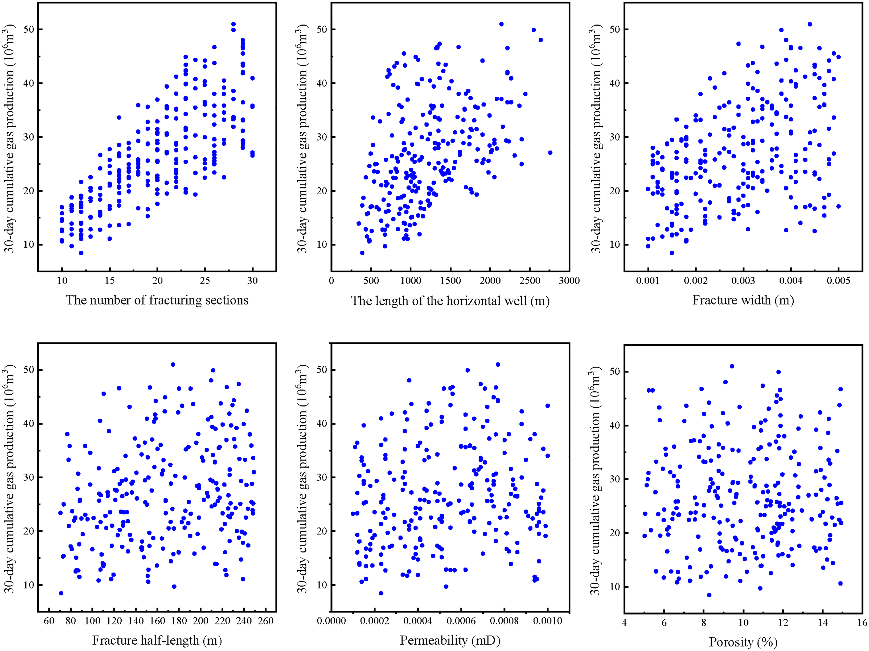
The distribution plots between the input parameters and output parameter. The input parameters are porosity, permeability, the number of fracturing sections, the length of the horizontal well, fracture width, and fracture half-length. The output is the 30-day cumulative gas production.

Building the productivity prediction model

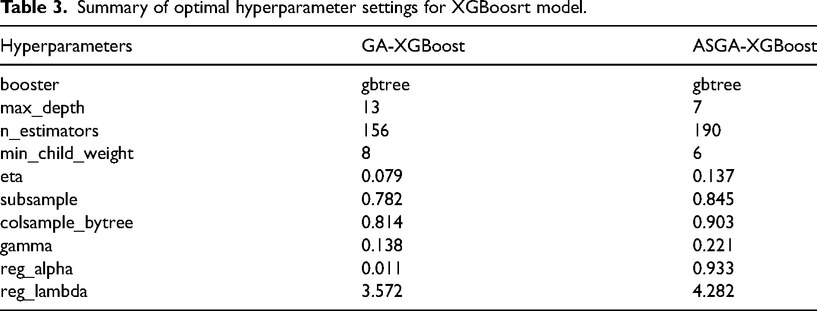
For the production prediction model established by the XGBoost algorithm, the input has six parameters, including porosity, permeability, the number of fracturing sections, the length of the horizontal well, fracture width, fracture half-length, and the output is the 30-day cumulative gas production. In this study, 80% of the samples from the dataset above were randomly selected as the training set, and the remaining 20% were used as the testing set. The training set was used to train the XGBoost model. In the process, 10% of samples from the training set were used as the validation set to achieve the 10-fold cross-validation, which is beneficial for obtaining a stable and accurate XGBoost model. The validation accuracy could represent the training accuracy of the XGBoost model. To improve the performance of the XGBoost model, ASGA was used to optimize the hyperparameters of the XGBoost model. Furthermore, to test the superiority of ASGA, GA was applied to the hyperparameter optimization and the comparison results are shown in Figure 5. As can be seen, the number of iterations used by ASGA to reach the optimal training accuracy is less than that of GA, and the training accuracy of the XGBoost model optimized by ASGA is 2.28% higher than that of GA. Thus, ASGA has a faster optimization speed and higher accuracy than GA. More precisely, the hyperparameters optimized by ASGA and GA are shown in Table 3.

Figure 5.

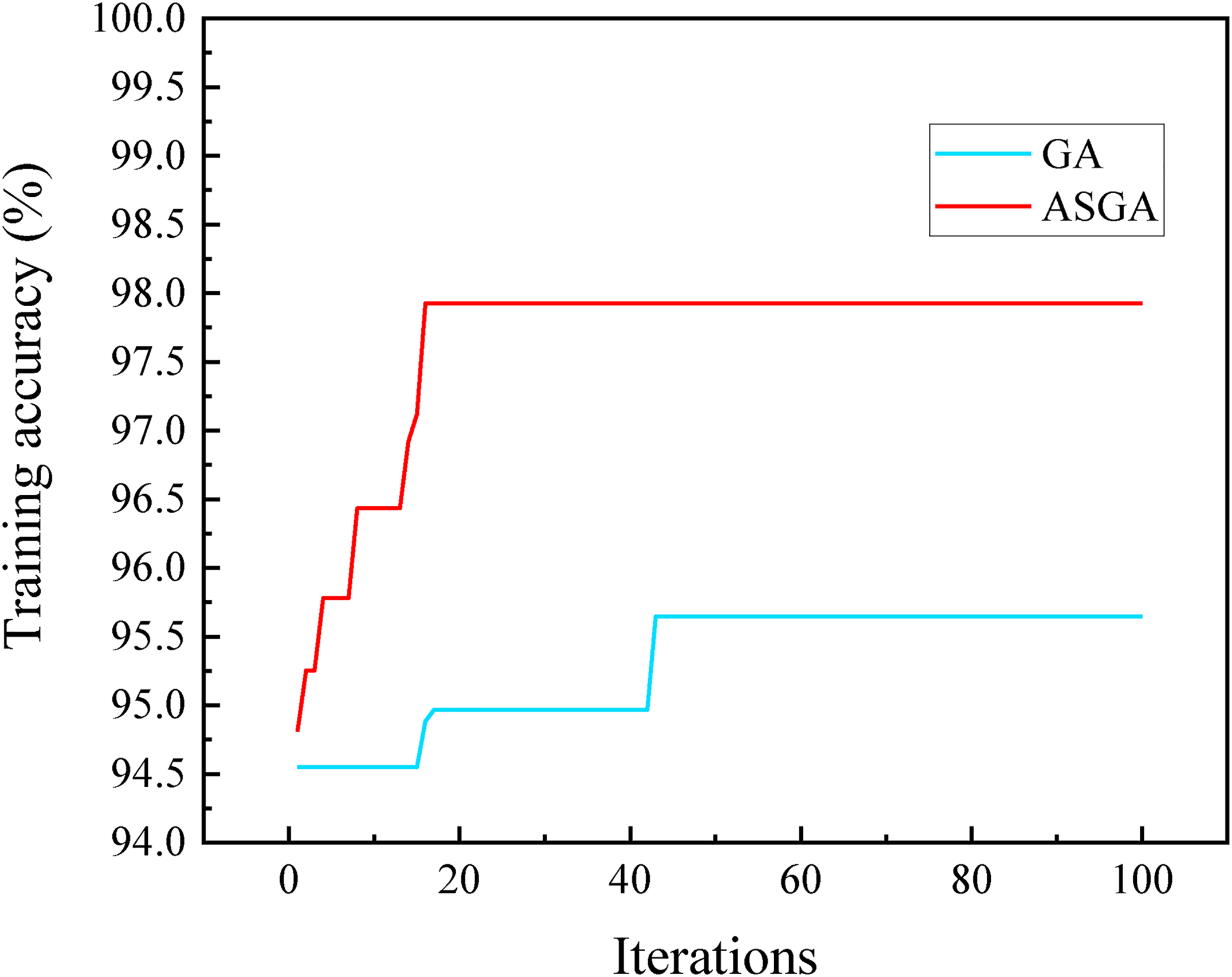
Comparison plots of GA vs. ASGA. The horizontal axis represents the iterations in the optimization process, and the vertical axis denotes the training accuracy of the XGBoost model. The light blue line denotes the optimization process of GA, and the red line represents the optimization process of ASGA.

Table 3.

Summary of optimal hyperparameter settings for XGBoosrt model.

Hyperparameters	GA-XGBoost	ASGA-XGBoost
booster	gbtree	gbtree
max_depth	13	7
n_estimators	156	190
min_child_weight	8	6
eta	0.079	0.137
subsample	0.782	0.845
colsample_bytree	0.814	0.903
gamma	0.138	0.221
reg_alpha	0.011	0.933
reg_lambda	3.572	4.282

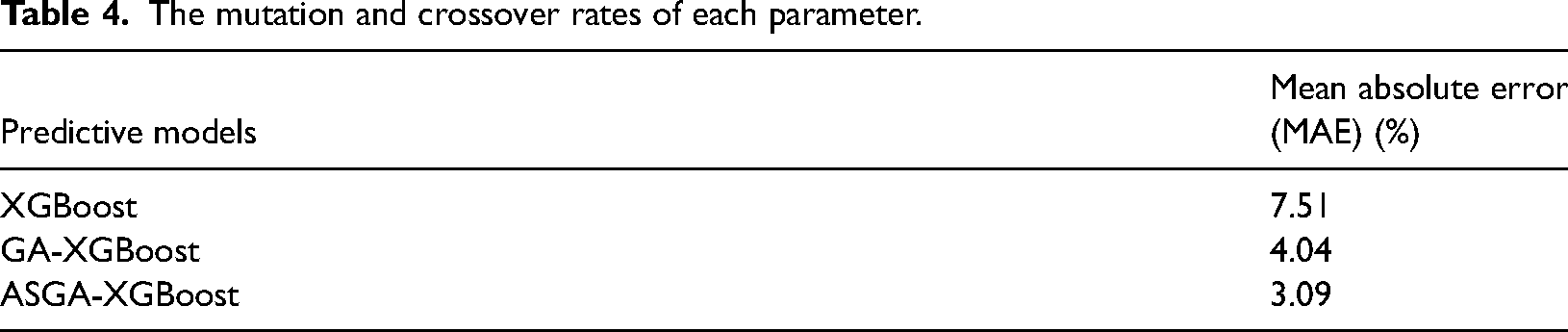
In addition, the samples in the testing set were used to validate the prediction performance of the XGBoost model optimized by ASGA. Moreover, the unoptimized XGBoost model and the XGBoost model optimized by GA were also used to predict the 30-day cumulative gas productions of the samples in the testing set, and the results are shown in Figure 6. As can be seen, the prediction results of the GA-XGBoost and ASGA-XGBoost models are better than that of the XGBoost model. More precisely, mean absolute error (MAE) was calculated to show the performance of the three models, and the result is shown in Table 4. It shows that the MAEs of XGBoost, GA-XGBoost, and ASGA-XGBoost are 7.51%, 4.04%, and 3.09%, respectively. Therefore, ASGA-XGBoost performs best in predicting the 30-day cumulative gas production. Furthermore, it also can be seen that the XGboost models optimized by intelligent optimization algorithms perform better than the XGboost model without optimization.

Figure 6.

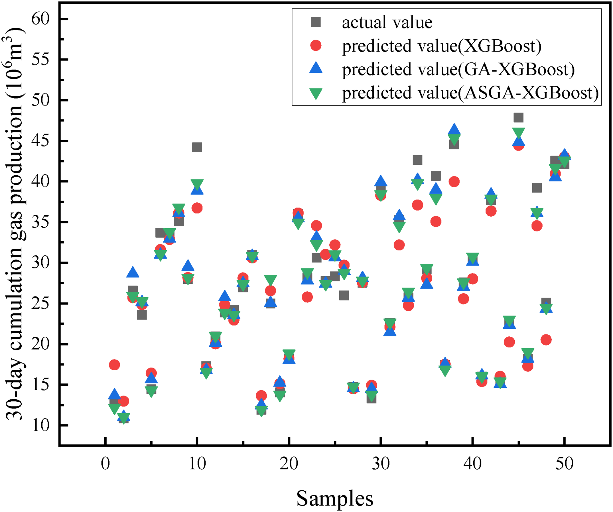
Comparison plots of actual values vs. predicted values for the validation samples. The black points denote the actual values, and the red points represent the values predicted by the XGBoost model. The blue points are the values predicted by the GA-XGBoost model, and the green points denote the values predicted by the ASGA-XGBoost model.

Table 4.

The mutation and crossover rates of each parameter.

Predictive models	Mean absolute error (MAE) (%)
XGBoost	7.51
GA-XGBoost	4.04
ASGA-XGBoost	3.09

Summary and conclusion

In this study, the researchers applied the ASGA-XGBoost model to predict the 30-day cumulative gas production of a shale gas horizontal well. The ASGA algorithm was employed to optimize the hyperparameters of the XGBoost model, leading to improved prediction accuracy. To evaluate the ASGA-XGBoost performance, a dataset was obtained through the establishment of a numerical simulation model of shale gas horizontal well fracturing using the CMG commercial numerical simulation software. Moreover, GA-XGBoost and XGBoost models were also employed in predicting the 30-day cumulative gas production. On the basis of the achieved results, the following conclusions can be drawn:

(1) Compared with GA, ASGA performs better in optimizing the hyperparameters of the XGBoost model. The optimization results show that the number of iteration steps of ASGA used for searching the optimal hyperparameters is less than that of GA, and the optimization accuracy of ASGA is higher than that of GA.

(2) ASGA-XGBoost performs better than GA-XGBoost and XGBoost in predicting the 30-day cumulation gas production. The results show that the MAEs of XGBoost, GA-XGBoost, and XGBoost are 7.51%, 4.04%, and 3.09%, respectively. It also can be seen that the MAE of the XGBoost model that has not been optimized is significantly higher than that of the optimized XGBoost model, which means that the XGboost model optimized by intelligent optimization algorithm performs better than the XGboost model without optimization.

(3) The weakness of this study is that the parameters obtained from numerical simulation are not comprehensive enough. This may limit the application of the ASGA-XGBoost model in the field. Furthermore, it is vital to acknowledge that the Spearman correlation coefficient only presents an approximate depiction of correlation. Such limitations may constrain ASGA's optimization accuracy and subsequently impact the prediction precision of ASGA-XGBoost.

Footnotes

Author contributions

Xin Zhou contributed to the conceptualization, methodology, software, testing, formal analysis, investigation, data curation, experimental studies, writing—original draft preparation, writing—reviewing and editing. Qiquan Ran contributed to the conceptualization, resources, data curation, data acquisition, writing—original draft preparation, writing—reviewing and editing, visualization, supervision, project administration.

Declaration of conflicting interests

The author(s) declared no potential conflicts of interest with respect to the research, authorship, and/or publication of this article.

Funding

The author(s) disclosed receipt of the following financial support for the research, authorship, and/or publication of this article: This research was funded by [Key Core Technology Research Projects of PetroChina Company Limited] grant number [2020B-4911]. And the APC was funded by [Research Institute of Petroleum Exploration and Development].

ORCID iD

Xin Zhou

Appendix

References

Abdul

Tze-Haw

Alexey

, et al. (2021) Are the responses of sectoral energy imports asymmetric to exchange rate volatilities in Pakistan? Evidence from recent foreign exchange regime. Frontiers in Energy Research 9: 614463. https://doi.org/10.3389/fenrg.2021.614463.

Alexey

Hasan

Serhat

(2023) Analysis of financial development and open innovation oriented fintech potential for emerging economies using an integrated decision-making approach of MF-X-DMA and golden cut bipolar q-ROFSs. Financial Innovation 9: 4.

Barnes

Bosworth

(2015) LNG Is linking regional natural gas markets: Evidence from the gravity model. Energy Economics 47: 11–17.

Bhuiyan

Zhang

Khare

, et al. (2022) Renewable energy consumption and economic growth nexus—A systematic literature review. Frontiers in Environmental Science 10: 878394. https://doi.org/10.3389/fenvs.2022.878394.

Chen

Guestrin

(2016) XGBoost: A scalable tree boosting system. Presented at the 22nd ACM SIGKDD International Conference on Knowledge Discovery and Data Mining (KDD). San Francisco, CA, AUG 13-17, 2016.

Chen

Gao

, et al. (2022) Prediction of shale gas horizontal wells productivity after volume fracturing using machine learning—an LSTM approach. Petroleum Science and Technology 40(15): 1861–1877.

Cheng

Yang

(2021) Prediction of oil well production based on the time series model of optimized recursive neural network. Petroleum Science and Technology 39(9-10): 303–312.

Chris

(2020) Dynamometer-Card classification uses machine learning. Journal of Petroleum Technology 72(3): 52–53.

Cossio

Moridis

GJJ

Blasingame

TAA

(2013) A semianalytic solution for flow in finite-conductivity vertical fractures by use of fractal theory. SPE Journal 18(01): 83–96.

10.

David

Anthony

Jude

(2022) Application of genetic algorithm on data driven models for optimized ROP prediction. Presented at the SPE Nigeria Annual International Conference and Exhibition, Lagos, Nigeria, August 2022. https://doi.org/10.2118/212016-MS

11.

Guo

, et al. (2017) Geological factors controlling shale gas enrichment and high production in fuling shale gas field. Petroleum Exploration and Development 44(4): 513–523.

12.

Hasan

Serhat

Alexey

, et al. (2022) Analysis of environmental priorities for green project investments using an integrated q-rung orthopair fuzzy modeling. IEEE Access 10: 50996–51007.

13.

Zhang

Rui

, et al. (2016) Fractured horizontal well productivity prediction in tight oil reservoirs. Journal of Petroleum Science & Engineering 151: 159–168.

14.

Irani

Shahbazian

Nasimi

(2011) Permeability estimation of a reservoir based on neural networks coupled with genetic algorithms. Petroleum Science and Technology 29(20): 2132–2141.

15.

John

(1992) Adaptation in Natural and Artificial Systems. Cambridge., MA: MIT Press: U.S. ISBN 978-0262581110.

16.

Karen

(2005) Optimizing cyclic-steam oil production with genetic algorithms. Journal of Petroleum Technology 57(06): 68–69.

17.

Kulgaa

Artunb

Ertekin

(2017) Development of a data-driven forecasting tool for hydraulically fractured, horizontal wells in tight-gas sands. Computers & Geosciences 103: 99–110.

18.

Serhat

Hasan

(2022) Bipolar q-ROF hybrid decision making model with golden cut for analyzing the levelized cost of renewable energy alternatives. IEEE Access 10: 42507–42517.

19.

Wang

Liu

, et al. (2021) Per-capita carbon emissions in 147 countries: The effect of economic, energy, social, and trade structural changes. Sustainable Production and Consumption 27: 1149–1164.

20.

Liang

Lou

Zhang

, et al. (2012) The first real time reservoir characterization, well placement and RSS applications in shale gas horizontal well play in Central China—A case study. Presented at the IADC/SPE Asia Pacific Drilling Technology Conference and Exhibition, Tianjin, China, July 2012. https://doi.org/10.2118/156239-MS

21.

Lin

Zhao

, et al. (2022) Productivity model of shale gas fractured horizontal well considering complex fracture morphology. Journal of Petroleum Science & Engineering 208: 109511.

22.

Lin

Ren

Zhao

(2018) Cluster spacing optimization for horizontal-well fracturing in shale gas reservoirs: Modeling and field application. Presented at the SPE Europec featured at 80th EAGE Conference and Exhibition, Copenhagen, Denmark, June 2018. https://doi.org/10.2118/190775-MS

23.

Liu

Zhang

(2014) Oil production prediction with neural network method. International Conference on Computer Science & Service System 2014.

24.

Liu

(2020) Predictive model for water absorption in sublayers using a Joint Distribution Adaption based XGBoost transfer learning method. Journal of Petroleum Science and Engineering 188: 106937.

25.

Mirzaei-Paiaman

Salavati

(2012) The application of artificial neural networks for the prediction of oil production flow rate. Energy Sources Part A-Recovery Utilization and Environmental Effects 34(19): 1834–1843.

26.

Najibi

Rezaei

Javanmardi

, et al. (2009) Economic evaluation of natural gas transportation from Iran's South-Pars gas field to market. Applied Thermal Engineering 29(10): 2009–2015.

27.

Nasimi

Irani

Ashena

(2012) Optimized scenario for bottomhole pressure prediction in underbalanced drilling based on neural networks coupled with particle swarm optimization. Petroleum Science and Technology 30(11): 1140–1150.

28.

Paul

Piroska

Saud

, et al. (2019) A fractal approach to the modelling and simulation of heterogeneous and anisotropic reservoirs. Presented at the SPE Offshore Europe Conference and Exhibition, Aberdeen, UK, September 2019. https://doi.org/10.2118/195778-MS

29.

Reymond

(2007) European key issues concerning natural gas: Dependence and vulnerability. Energy Policy 35(8): 4169–4176.

30.

Song

Jiang

, et al. (2017) Progress and development trend of unconventional oil and gas geological research. Petroleum Exploration and Development 44(4): 675–685.

31.

Souza

RMS

Coelho

Santos

AAS

, et al. (2018) Search operators for genetic algorithms applied to well positioning in oil fields. 7th Brazilian Conference On Intelligent Systems (BRACIS). 498-503. DOI:https://doi.org/10.1109/BRACIS.2018.00092

32.

Tang

Fan

Xiao

, et al. (2021) A new ensemble machine-learning framework for searching sweet spots in shale reservoirs. SPE Journal 26(01): 482–497.

33.

Umbach

(2013) The unconventional gas revolution and the prospects for Europe and Asia. Asia Europe Journal 11(3): 305–322.

34.

Wang

Zhou

Fan

, et al. (2016) Utilising managed pressure drilling to drill shale gas horizontal well in fuling shale gas field. Presented at the SPE Asia Pacific Oil & Gas Conference and Exhibition, Perth, Australia, October 2016. https://doi.org/10.2118/182490-MS

35.

Wang

Lin

(2014) Impacts of unconventional gas development on China's natural gas production and import. Renewable & Sustainable Energy Reviews 39: 546–554.

36.

Wang

Shi

, et al. (2022) Productivity prediction of fractured horizontal well in shale gas reservoirs with machine learning algorithms. Applied Sciences-Basel 11(24): 12064.

37.

Wathiq

Maytham

(2011) Adopting simple & advanced genetic algorithms as optimization tools for increasing oil recovery & NPV in an Iraq oil field. SPE-140538-MS. https://doi.org/10.2118/140538-MS

38.

Yuan

Yan

Chen

, et al. (2018) Numerical simulation for shale gas flow in complex fracture system of fractured horizontal well. International Journal of Nonlinear Sciences and Numerical Simulation 19(3-4): 367–377.

39.

Zhang

Jiang

Chen

, et al. (2015) A newly developed rate analysis method for a single shale gas well. Energy Exploration & Exploitation 33(3): 309–316.

40.

Zhou

Ran

(2023) Optimization of fracturing parameters by modified genetic algorithm in shale gas reservoir. Energies 16(6): 2868.

Production prediction based on ASGA-XGBoost in shale gas reservoir

Abstract

Keywords

Introduction

Methodology

XGBoost algorithm

ASGA-XGBoost model

Application

Data description

Building the productivity prediction model

Summary and conclusion

Footnotes

Author contributions

Declaration of conflicting interests

Funding

ORCID iD

Appendix

References