Sage Journals: Discover world-class research

Abstract

Traditional machine learning methods are difficult to accurately forecast oil production when development measures change. A method of oil reservoir production prediction based on normalized mutual information and a long short-term memory-based sequence-to-sequence model (Seq2Seq-LSTM) was proposed to forecast reservoir production considering the influence of liquid production and well spacing density. First, the marine sandstone reservoirs in the Y basin were taken as the research object to establish the sample database. Then, the feature selection was carried out according to the normalized mutual information, and liquid production, production time, equivalent well spacing density, fluidity and original formation pressure were determined as input features. Finally, a Seq2Seq-LSTM model was established to forecast reservoir production by learning the interaction from multiple samples and multiple sequences, and mining the relationship between oil production and features. The research showed that the model has a high accuracy of production prediction and can forecast the change of production when the liquid production and well spacing density change, which can provide scientific recommendations to help the oilfield develop and adjust efficiently.

Keywords

Machine learning production prediction normalized mutual information long short-term memory-based sequence to sequence model liquid production well spacing density

Introduction

The development of oil and gas resources has an important impact on a country's energy security and economic development (Ullah et al., 2022). Changing well spacing density and adjusting liquid production are the most popular development measures to control oil production in reservoirs. It is very important for the adjustment and formulation of the reservoir development plan to forecast oil production considering the influence of liquid production and well spacing density. Decline curve analysis (DCA), numerical reservoir simulation, analytical methods and machine learning are widely used to predict the oil and gas production of reservoirs.

DCA is an empirical formula for determining production changes by regression of oil and gas production data, without the help of relevant data on reservoir physical properties. Arps (1945) proposed the simplest empirical DCA method, which has been universally used for conventional reservoirs. Many scholars modified the traditional Arps’ decline model and thus proposed the Power Law Exponential decline model and the Stretched Exponential Decline Model (Ilk et al., 2008; Valko, 2009). The technique of DCA can roughly characterize the variation of reservoir production, but can’t consider the influence of development measures on oil and gas production. Numerical reservoir simulation is to simulate the underground oil and water flow by establishing and solving the reservoir geological and numerical models, and giving the distribution of oil and water at a certain time to predict the reservoir dynamics (Gao et al., 2016; Yang et al., 2021; Zhang and Awotunde, 2016). If the accuracy of numerical simulation to predict production is high, it often needs to invest considerable time and effort. Therefore, it is a formidable task to establish an accurate and practical numerical model. The analytical method uses a lot of assumptions to establish a mathematical model (Liu et al., 2017; Sang et al., 2014; Wang et al., 2020b). Compared with numerical reservoir simulation, the analytical method has the advantage of faster calculation speed, but the simplified model has limited practicability. The oil and gas production of reservoirs is mainly influenced by geological parameters, fluid properties and development measures. It is difficult for traditional methods to accurately forecast oil production because of the complex nonlinear relationship between various factors and production.

After years of development, a large amount of production data has been accumulated in a reservoir, which provides the basis for the application of machine learning (ML). The applicability of ML in various domains of petroleum engineering has attracted extensive attention and interest. Vector autoregression (Zhang and Jia, 2021), support vector regression (Huang et al., 2021; Masoud et al., 2020), random forest (Bhattacharya et al., 2019; Xue et al., 2021) and artificial neural network (Liu et al., 2021b; Negash and Yaw, 2020; Zhang et al., 2016; Zhou et al., 2021b) are used to predict oil and gas production. However, these traditional ML methods do not take into account the trend of production over time and the correlation between the data before and after.

In order to improve prediction accuracy, a deep learning method called long short-term memory (LSTM) network has been popularly used to forecast oil production. Sagheer and Kotb (2018) established a deep LSTM architecture to predict production data from North China Oilfield in China and Cambay Basin Oilfield in India. Wang et al. (2020a) used the production data of waterflooding sandstone reservoirs to establish the production prediction model by the LSTM network, which can predict the production of ultra-high water cut period. Yang and Wang (2020) presented a novel optimization method that integrates the LSTM neural network and dynamic programming to solve the optimization problem of SAGD steam injection volume innovatively. Bao et al. (2020) used ensemble Kalman filter enhanced LSTM to establish a data-driven end-to-end model for forecasting production, which can forecast future water content and oil production by inputting injection rate, bottom hole pressure, previous water content and oil production. Xu et al. (2020) proposed a transfer-LSTM production prediction model of coalbed methane, which combined the idea of transfer learning and the LSTM model. Song et al. (2020) optimized the structure and parameters of the LSTM model by particle swarm optimization algorithm and established the production forecasting model of fractured horizontal wells in volcanic reservoirs. Liu et al. (2020) proposed an LSTM model based on ensemble empirical mode decomposition, which can accurately predict the oil production of wells. Dong et al. (2021) first used well groups with sufficient historical data to train the LSTM model, and then the model combined with transfer learning was applied to the production prediction of the well group with a short development time in the same oilfield. Guo et al. (2021) extracted features by combining convolutional autoencoder and spatial pyramid pooling and established the coalbed methane production prediction model based on LSTM. Rodriguez and Salazar (2022) used LSTM neural network to forecast oil and water production in an oil field exploited through waterflooding, which can change input parameters such as bottom hole pressure or water injection rate to predict production. Zhang et al. (2022) used a temporal convolutional network (TCN) to predict the oil production of a single well in water flooding reservoirs at different water cut stages. Du et al. (2023) established a data-driven production forecasting model for coalbed methane based on Bi-LSTM.

The above models are only are only trained to predict the production of one well or one reservoir, referred to as ‘single-series learning’. In the same oilfield, there is a certain similarity between each well or each reservoir. If the neural network is able to train multiple related time series and samples altogether in one lumped model, it can not only learn the variation of time series, but also learn the relationship between target variable and features from multiple samples and multiple sequences. This neural network is called ‘cross-series learning’, which can simultaneously predict multiple target variables. At present, this neural network model has been applied to forecast weather, temperature and other fields (Castro et al., 2021; Fang et al., 2021; Javier et al., 2021; Zaytar and Amrani, 2016).

In this study, an LSTM-based sequence-to-sequence model (Seq2Seq-LSTM) driven by reservoir spatial-temporal data was proposed to forecast the oil production of reservoirs in response to the limitations of existing machine learning in predicting oil production. The traditional LSTM models cannot forecast production under the influence of well spacing density and liquid production. The Seq2Seq-LSTM network is employed to learn the interaction from multiple samples and multiple sequences and explores the relationship between oil production and features, such as reservoir properties and development measures. The proposed model can accurately forecast the oil production when the liquid production and well spacing density change, which can provide scientific recommendations to help the oilfield develop and adjust efficiently.

Methodology

Modelling steps

In this work, a method of oil reservoir production prediction based on spatial–temporal data and Seq2Seq-LSTM was proposed to forecast reservoir production considering the influence of liquid production and well spacing density. This method follows the flowchart shown in Figure 1. Next, the modelling steps are elaborated based on the flowchart.

Some reservoirs in the target area are selected as samples to collect the historical production data and the parameters of reservoir physical properties, including oil production, liquid production, production time, number and type of development wells, original formation pressure, reservoir thickness, reservoir area, porosity, heterogeneity and fluidity, and extract the time series of relevant parameters of each reservoir.

On the one hand, since the reservoirs in the target area are jointly developed by horizontal wells and vertical wells, in order to standardize and quantify different well types, it is essential to convert the horizontal wells into the equivalent number of vertical wells to obtain the equivalent well spacing density. On the other hand, data normalization is carried out to reduce the adverse impact on model training caused by dimensional differences.

Normalized mutual information is used to evaluate the correlation between the feature series and oil production series, and features with strong correlations are imported into the model.

The data are divided into training set and testing set. Based on the training set, the structure and parameters of the Seq2Seq-LSTM model are defined and optimized by a genetic algorithm (GA).

Based on the trained model and testing set, the oil production of reservoirs considering the influence of liquid production and well spacing density is predicted to verify the accuracy of the model.

Figure 1.

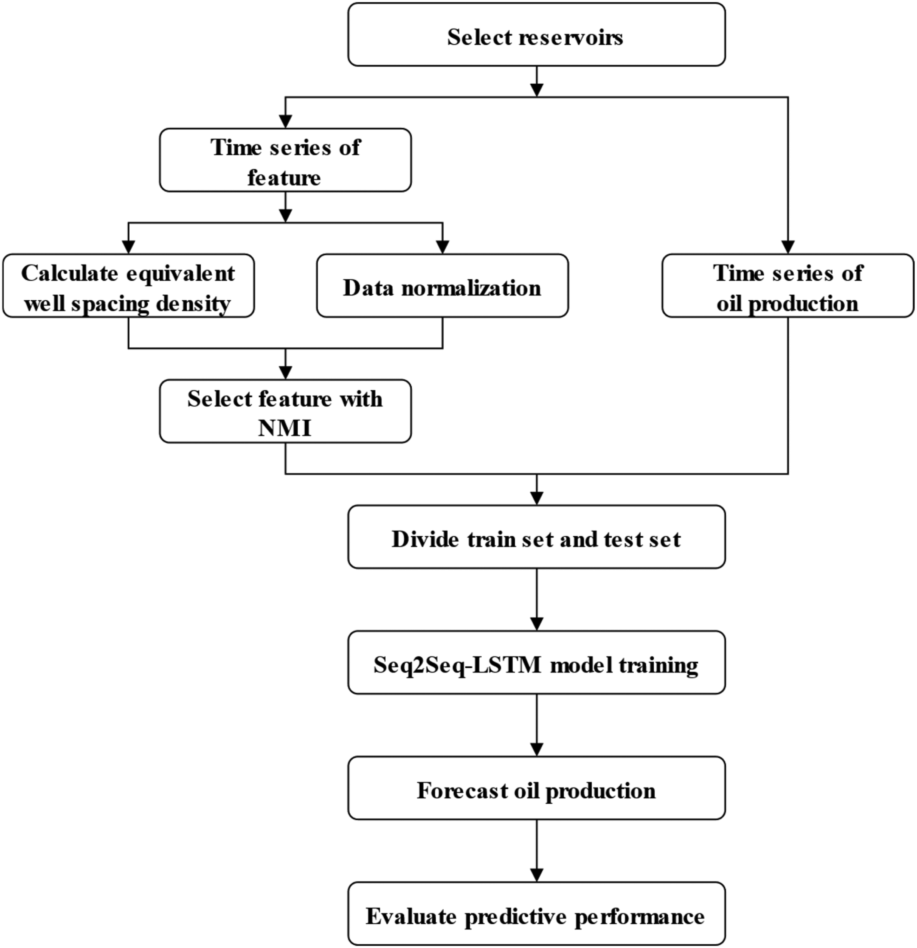
Workflow of the production prediction driven by reservoir spatial–temporal data.

Normalized mutual information

It is very important to select the main features affecting reservoir production, which is helpful to improve the generalization ability and prediction accuracy of the model. The input variable selection is accomplished through normalized mutual information (NMI). NMI is adopted as the similarity measure, as equation (1), which measures how much information, on average, one random variable provides to another (Danon et al., 2006; Liu et al., 2021a; Zhou et al., 2021a). The advantage of NMI is that it can measure the nonlinear relationship between variables.

U (X, Y) = \frac{- 2 \sum_{y \in Y} \sum_{x \in X} p (x, y) \log_{b} (\frac{p (x, y)}{p (x) p (y)})}{\sum_{x \in X} p (x) \log_{b} p (x) + \sum_{y \in Y} p (y) \log_{b} p (y)}

(1)

where X is the feature time series; Y is the target time series; p(x) is the marginal probability function of feature value x; p(y) is the marginal probability function of target value y; p(x, y) is the joint probability function of x and y.

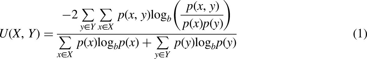
According to the definition of NMI, when U(X, Y) = 0, it shows that X and Y are independent of each other, that is, zero correlation; the larger the value of U(X, Y), the stronger the correlation between X and Y; when U(X, Y) = 1, it shows that X and Y are complete correlation. The value of NMI between each feature and the target is calculated by equation (1), and sorted in descending order. Finally, the first k features are imported into the model.

Long short-term memory

Long short-term memory (LSTM) is a special kind of RNN, capable of learning long-term dependencies (Hochreiter and Schmidhuber, 1997). LSTM is explicitly designed to avoid the long-term dependency problem. LSTM adds a new internal state c_t to transmit circular information in linear mode, and then transmits information in nonlinear mode to the external state h_t of the hidden layer. Computing processes are demonstrated as

c_{t} = f_{t} ⊙ c_{t - 1} + i_{t} ⊙ {\tilde{c}}_{t}

(2)

h_{t} = o_{t} ⊙ \tanh (c_{t})

(3)

where f_t is the ‘forget gate’ that determines what information can pass through the cell state; i_t is the ‘input gate’ that determines which values should be updated; o_t is the ‘output gate’, deciding what to output; ⊙ is element-wise product; c_t−₁ is the cell state at the previous moment; c͂_t is a vector of new candidate value. These can be formulated as

f_{t} = σ (W_{f} x_{t} + U_{f} h_{t - 1} + b_{f})

(4)

i_{t} = σ (W_{i} x_{t} + U_{i} h_{t - 1} + b_{i})

(5)

o_{t} = σ (W_{o} x_{t} + U_{o} h_{t - 1} + b_{o})

(6)

{\tilde{c}}_{t} = \tanh (W_{c} x_{t} + U_{c} h_{t - 1} + b_{c})

(7)

where σ(·) is the logistic function, which generates a 0 to 1 value; x_t is the current input; h_t−₁ is the output at the previous moment; W and U are the weights; b is the bias term.

A schematic diagram of the LSTM network is shown in Figure 2. First, the three gates (f_t, i_t, o_t) and the candidate value c͂_t are calculated by using the output h_t−₁ at the previous moment and the input x_t at the current moment. Next, the cell state c_t is updated according to the ‘forget gate’ f_t and the ‘input gate’ i_t. Finally, the internal state c_t is processed by the tanh layer and then combined with the ‘output gate’ o_t to transmit data messages to the external state h_t.

Figure 2.

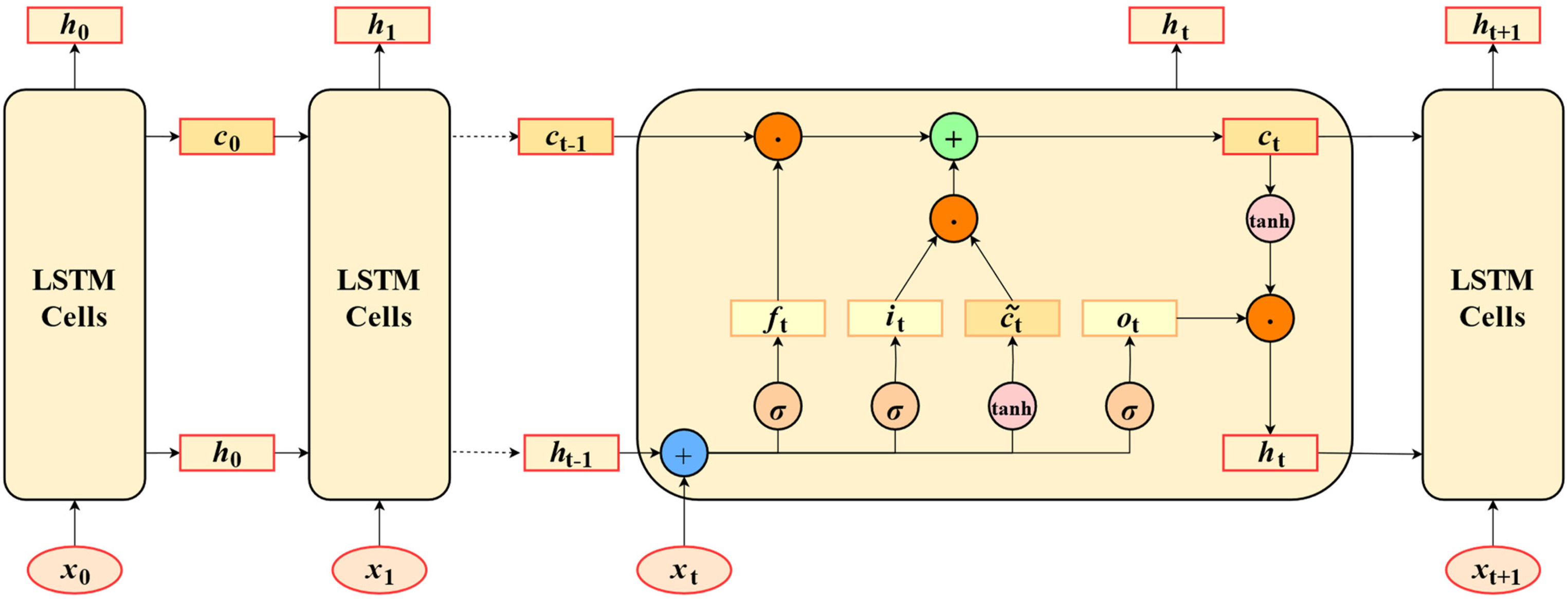
Schematic diagram of long short-term memory (LSTM) network.

LSTM-based sequence-to-sequence model

Seq2Seq-LSTM is an encoder–decoder neural network model composed of two LSTMs, which can realize the conversion from one sequence to another, taking into account the spatial–temporal dependence of multivariate time series data (Du et al., 2018). A schematic diagram of Seq2Seq-LSTM is shown in Figure 3. The model framework includes an encoder and decoder.

Figure 3.

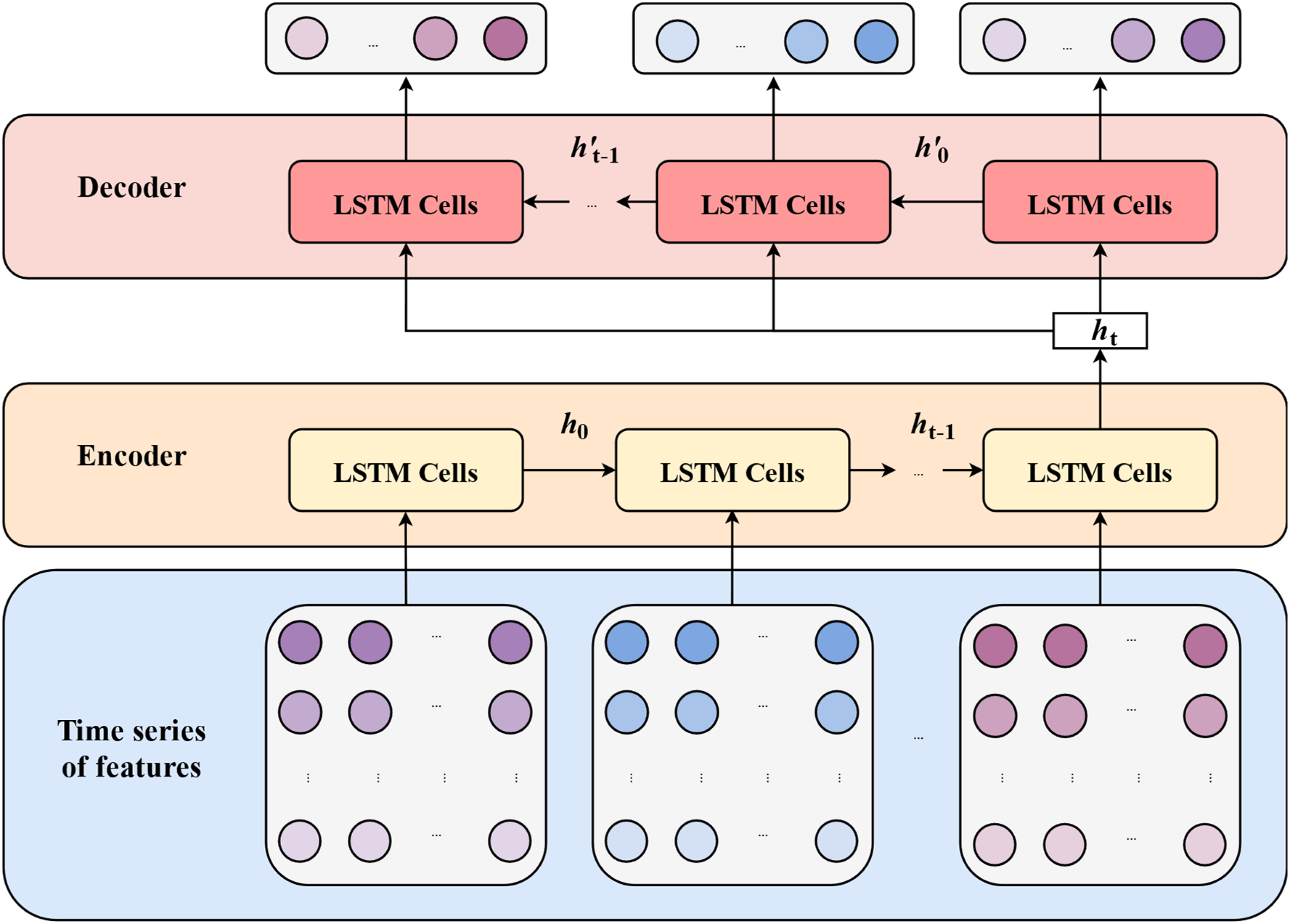
Schematic diagram of long short-term memory-based sequence-to-sequence model (Seq2Seq-LSTM).

The LSTM encoder takes n historical time series X₁, X₂, …, X_n with length T as imported data for learning and creates the fixed dimension vector u. u is the hidden state of the encoder at the last moment:

h_{t}^{enc} = f_{enc} (h_{t - 1}^{enc}, e_{X_{t - 1}}, θ_{enc})

(8)

u = h_{T}^{enc}

(9)

where e_X is the input feature vector; f_enc(·) is the LSTM encoder; θ_enc is network parameters.

When generating the target sequence, the LSTM decoder is used for decoding. At step t of the decoding process, the prefix sequence Y_1:(t−1) has been generated. $h_{t}^{d e c}$ represents the hidden state of the decoder:

h_{0}^{dec} = u

(10)

h_{t}^{dec} = f_{dec} (h_{t - 1}^{dec}, e_{Y_{t - 1}}, θ_{dec})

(11)

where e_Y is the output target vector; f_dec(·) is the LSTM decoder; θ_dec is network parameters.

For the prediction of reservoir production, oil production can be obtained by inputting the sequence of factors. The Seq2Seq-LSTM model driven by spatial-temporal data is to input all reservoir samples at the same time, and then learn the relationship between features and the oil production, so as to input a set of features and output a monthly oil production.

Database establishment

Data pre-processing

The marine sandstone reservoirs in the Y basin are taken as the research object. The structural differences of reservoirs in the Y basin are small, mainly low-amplitude anticline structure, no-fault, and high porosity and permeability. Each reservoir has its own independent oil–water system vertically. The reservoirs are developed by edge water or bottom water drive because of the strong water energy. The development time of these reservoirs is between 4 and 25 years, with complete and accurate historical production data and geological data. Most of the reservoirs are in the ultra-high water cut stage. Development wells in many reservoirs include horizontal wells and vertical wells at the same time. The development measures of these reservoirs are liquid production adjustment and well spacing density adjustment.

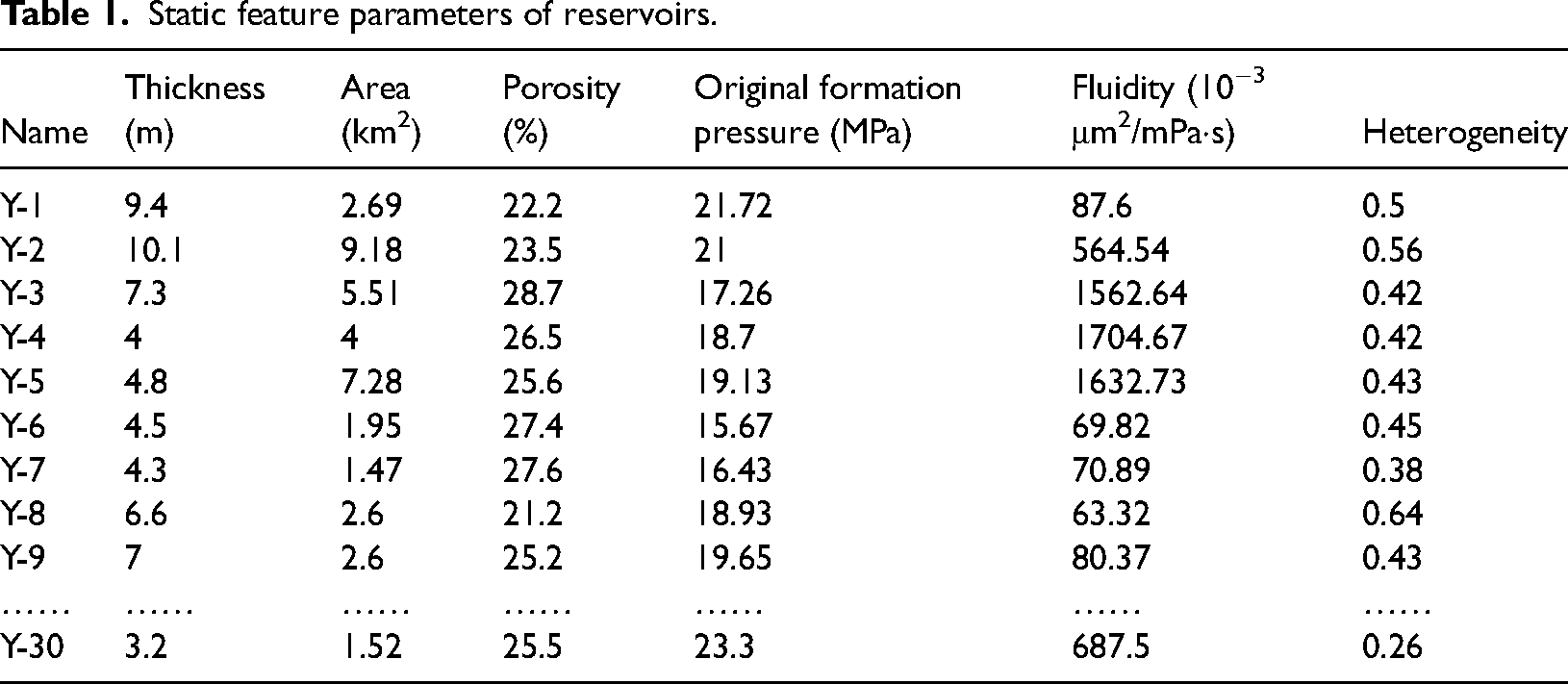
The 30 bottom water reservoirs in the Y basin are selected as samples to establish the database by sorting out and analysing the static and dynamic data of reservoirs. Sample selection observes the following principles: marine sandstone reservoirs developed by natural energy; same type of drive; similar oil property; accurate reservoir geological data and development data. According to the development experience of reservoirs, the parameters affecting oil production include static feature parameters and dynamic feature parameters. The static feature parameters include original formation pressure, reservoir thickness, reservoir area, porosity, heterogeneity and fluidity. The static feature parameters include production time, liquid production and well spacing density. Collect the above feature parameters and monthly oil production data of these 30 reservoirs from the beginning of development to January 2020. The static feature parameters of some reservoirs are shown in Table 1.

Table 1.

Static feature parameters of reservoirs.

Name	Thickness (m)	Area (km²)	Porosity (%)	Original formation pressure (MPa)	Fluidity (10⁻³ μm²/mPa·s)	Heterogeneity
Y-1	9.4	2.69	22.2	21.72	87.6	0.5
Y-2	10.1	9.18	23.5	21	564.54	0.56
Y-3	7.3	5.51	28.7	17.26	1562.64	0.42
Y-4	4	4	26.5	18.7	1704.67	0.42
Y-5	4.8	7.28	25.6	19.13	1632.73	0.43
Y-6	4.5	1.95	27.4	15.67	69.82	0.45
Y-7	4.3	1.47	27.6	16.43	70.89	0.38
Y-8	6.6	2.6	21.2	18.93	63.32	0.64
Y-9	7	2.6	25.2	19.65	80.37	0.43
……	……	……	……	……	……	……
Y-30	3.2	1.52	25.5	23.3	687.5	0.26

In order to determine the equivalent well spacing density of reservoirs, it is necessary to sort out the type, parameters and production time of each well in the reservoir. The number of different types of wells in the Y-1 reservoir and Y-2 reservoir changes with time, as shown in Figure 4.

Figure 4.

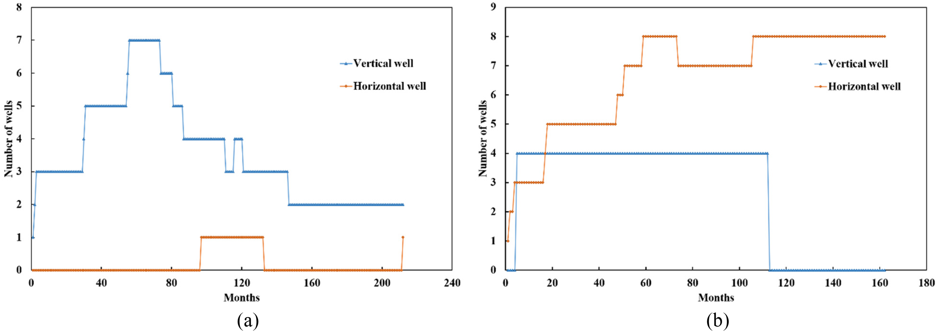
Type and number of development wells: (a) Y-1 reservoir; (b) Y-2 reservoir.

Since the reservoirs in the Y basin are jointly developed by horizontal wells and vertical wells, it is significant to convert the horizontal wells into the equivalent number of vertical wells to obtain the equivalent well spacing density so that different well types can be compared. In this work, the method of converting a horizontal well into vertical wells is based on the same total production and total control area. The equivalent number of vertical wells is calculated by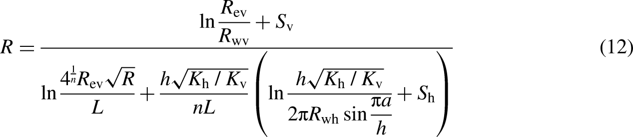

R = \frac{\ln \frac{R_{ev}}{R_{wv}} + S_{v}}{\ln \frac{4^{\frac{1}{n}} R_{ev} \sqrt{R}}{L} + \frac{h \sqrt{K_{h} / K_{v}}}{n L} (\ln \frac{h \sqrt{K_{h} / K_{v}}}{2 π R_{wh} \sin \frac{π a}{h}} + S_{h})}

(12)

where R is the number of vertical wells converted from a horizontal well; R_ev is the drainage radius of a vertical well, m; R_wv is the wellbore radius of a vertical well, m; R_wh is the wellbore radius of a horizontal well, m; S_v is the skin factor of the vertical well; S_h is the skin factor of the horizontal well; L is the horizontal section length of a horizontal well, m; n is the number of wellbores in the branch well; h is the effective thickness, m; K_h is the horizontal permeability, μm²; K_v is the vertical permeability, μm²; a is the distance from horizontal section of the horizontal well to bottom of reservoir, m.

After obtaining the total number of equivalent vertical wells in the target reservoir, the equivalent well spacing density of each reservoir can be calculated, given as follows:

D_{w} = \frac{W_{e}}{A}

(13)

where D_w is the equivalent well spacing density, well/km²; W_e is the total number of equivalent vertical wells; A is the reservoir area, km².

Taking Y-1 and Y-2 reservoirs as examples, the variation of equivalent well spacing density with time is calculated by equations (12) and (13), as shown in Figure 5.

Figure 5.

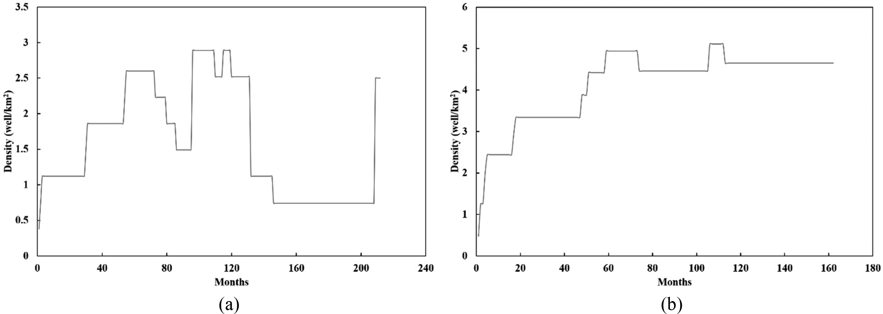
Equivalent well spacing density in the reservoir: (a) Y-1 reservoir; (b) Y-2 reservoir.

Data normalization is carried out to reduce the adverse impact on model training caused by differences in parameter units. Z-score standardization is selected in this study. The standardized parameters of this method are determined by

x_{n} = \frac{x - μ}{σ}

(14)

where x is the parameters to be standardized; μ is the mean value of variables; σ is the standard deviation of variables.

Feature selection based on normalized mutual information

Feature selection based on NMI is used to analyse the effect of each feature on monthly oil production. The results of the NMI of each feature sequence are shown in Figure 6.

Figure 6.

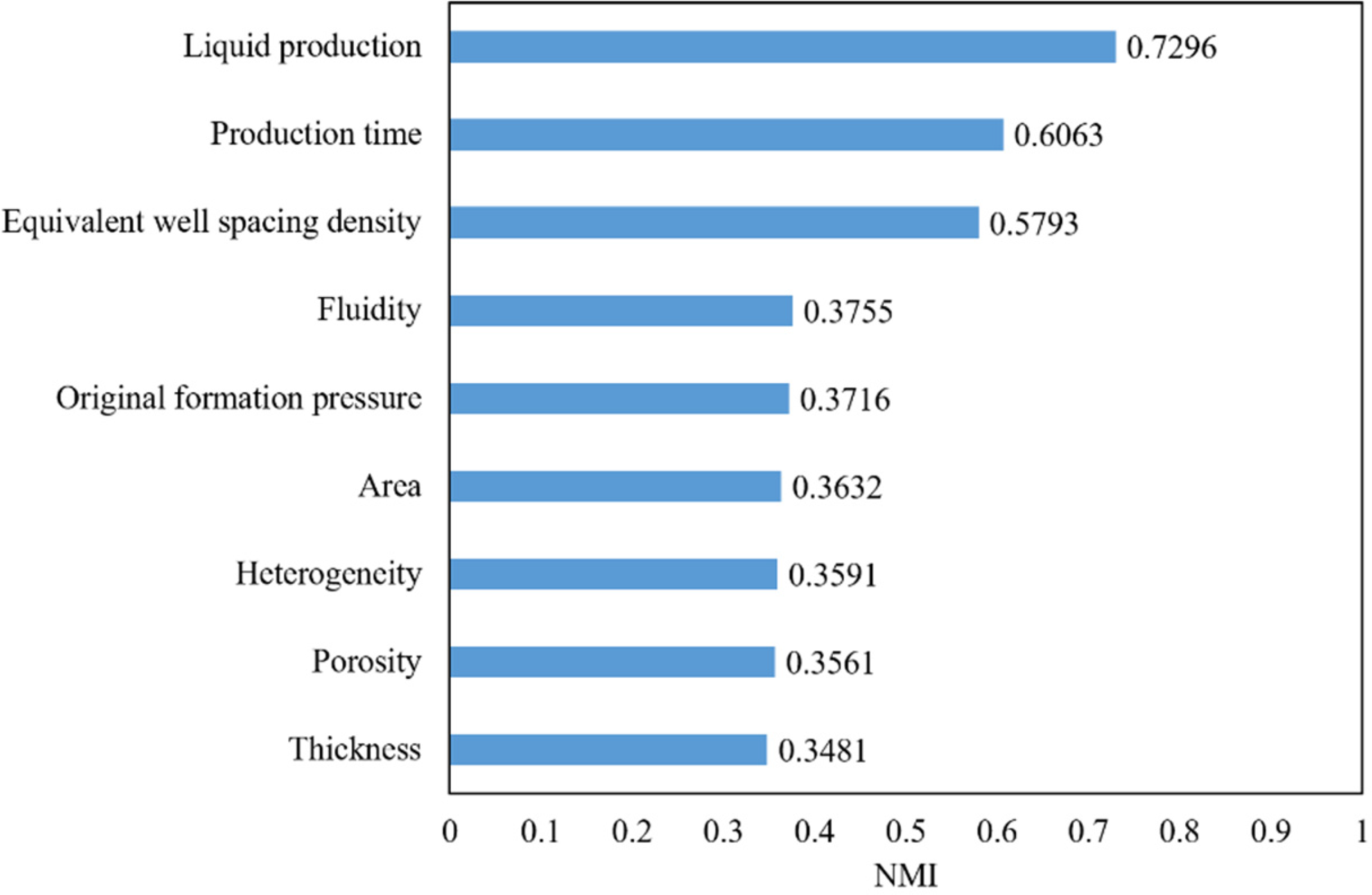
Calculation results of normalized mutual information (NMI).

The larger the value of NMI, the stronger the correlation between feature and oil production. According to the value of NMI from large to small, the correlation between feature and oil production from strong to weak is liquid production > production time > equivalent well spacing density > fluidity > original formation pressure > area > heterogeneity > porosity > thickness.

According to the ranking of NMI calculation results, the first k features are used as import data of the model. In this work, the first five features, which are liquid production, production time, equivalent well spacing density, fluidity, and original formation pressure, are selected as input of the model.

Modelling and application

Model training and structure optimizing

After the feature selection is completed, the prediction model of reservoir production can be established. Firstly, the original time series is divided into a training set and testing set on the basis of the ratio of 8.5:1.5. And then, Adam (Kingma and Ba, 2014) is adopted as a learning algorithm in this study. Adam algorithm can be regarded as the combination of the momentum method and RMSProp algorithm. It not only uses momentum as the parameter update direction, but also can adaptively adjust the learn rate.

Based on the Adam algorithm, the weights of the model are optimized by training the model continuously. Root mean square error (RMSE) is used to characterize the accuracy of the model, and its formula is as follows: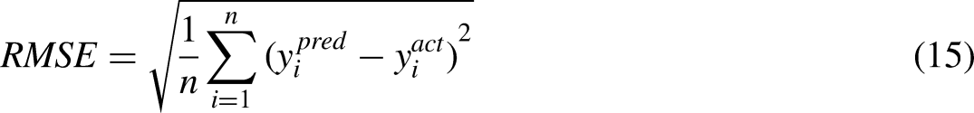

R M S E = \sqrt{\frac{1}{n} \sum_{i = 1}^{n} {(y_{i}^{p r e d} - y_{i}^{a c t})}^{2}}

(15)

where n is the length of the time series;

y_{i}^{p r e d}

is the predicted production, m³/month;

y_{i}^{a c t}

is the actual production, m³/month.

The hyper-parameters of the model are optimized by GA, which uses the random global searching algorithm to simulate the physical process of biological natural evolution, and can select, cross and mutate each individual randomly to search for the optimal solution. In this work, the coefficient of determination (R²) is used as the fitness function of GA.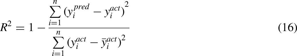

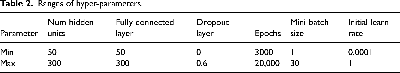
R^{2} = 1 - \frac{\sum_{i = 1}^{n} {(y_{i}^{p r e d} - y_{i}^{a c t})}^{2}}{\sum_{i = 1}^{n} {(y_{i}^{a c t} - {\bar{y}}_{i}^{a c t})}^{2}}

(16)

where

{\bar{y}}_{i}^{a c t}

is the average value of actual oil production, m³/month.

The hyper-parameters of the model include the number of hidden units, fully connected layer, dropout layer, epochs, mini-batch size and initial learn rate. Table 2 shows the ranges of hyper-parameters for models. The optimum hyper-parameters of the proposed model Seq2Seq-LSTM are shown in Table 3, which are optimized by GA.

Table 2.

Ranges of hyper-parameters.

Parameter	Num hidden units	Fully connected layer	Dropout layer	Epochs	Mini batch size	Initial learn rate
Min	50	50	0	3000	1	0.0001
Max	300	300	0.6	20,000	30	1

Table 3.

Obtained optimum hyper-parameters of Seq2Seq-LSTM based on GA.

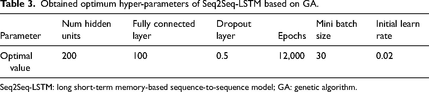
Parameter	Num hidden units	Fully connected layer	Dropout layer	Epochs	Mini batch size	Initial learn rate
Optimal value	200	100	0.5	12,000	30	0.02

Seq2Seq-LSTM: long short-term memory-based sequence-to-sequence model; GA: genetic algorithm.

Result verification

In this study, two reservoirs (Y-1 and Y-2 reservoirs) from the database are used to validate the proposed Seq2Seq-LSTM model. There is a total of 212 actual monthly oil production of the Y-1 reservoir and 162 actual monthly oil production of the Y-2 reservoir. The original series is divided on the basis of the ratio of 8.5:1.5 to obtain the training set and testing set, and the original oil production series, liquid production series, and equivalent well spacing density series are shown in Figure 7. According to Figure 7, the relationship between oil production, liquid production, and well spacing density can be understood intuitively. In general, the reservoirs developed by natural energy mainly adjust the oil production by changing liquid production and well spacing density. The oil production increased to varying degrees when the well spacing density or liquid production increased. In the Y-1 reservoir, the oil production in the 209th month increased, because the well spacing density and liquid production increased significantly. In the Y-2 reservoir, the oil production in the 113th-month oil production gradually decreased on the whole, because the well spacing density remained unchanged and the liquid production slightly decreased on the whole.

Figure 7.

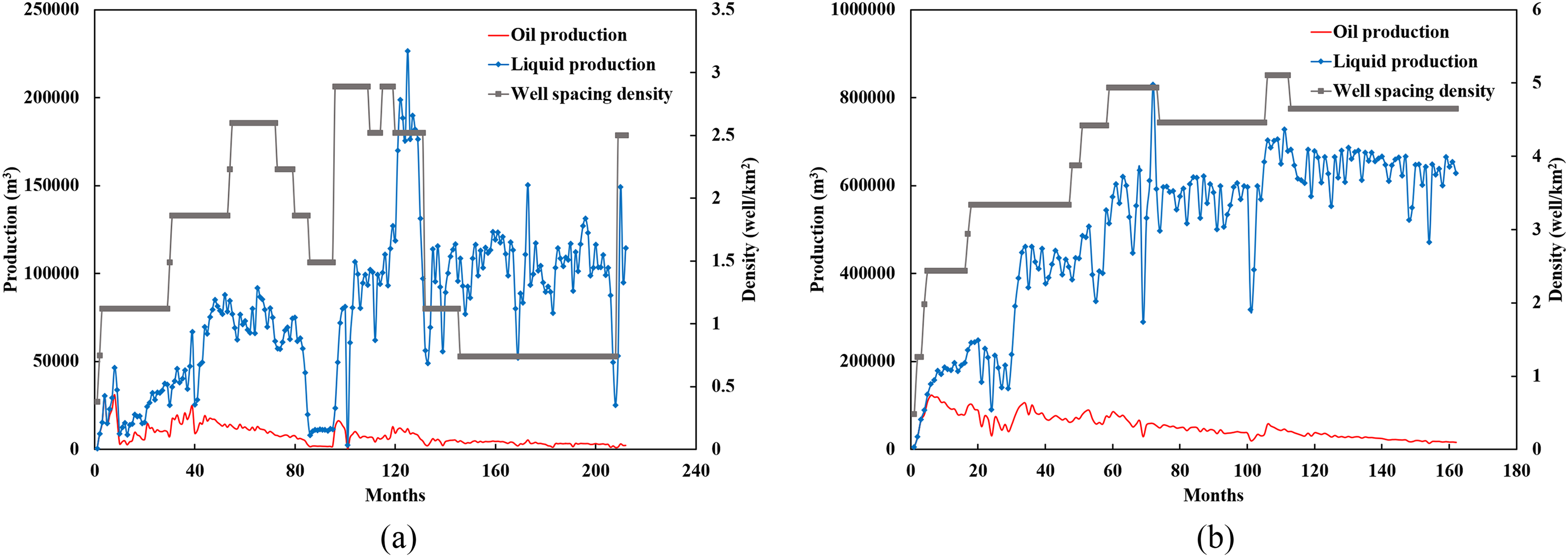
The original oil production, liquid production and equivalent well spacing density: (a) Y-1 reservoir; (b) Y-2 reservoir.

Figure 8 shows the prediction results of the proposed model, in which the actual oil production rate is compared with the predicted values using Seq2Seq-LSTM. It is clear that the oil production calculated by the proposed model is very close to the actual value. The data points of the training set and testing set are basically distributed near the 45° line (the closer to the 45° line, the smaller the deviation between the predicted value and the actual value). Based on the results, the proposed model can accurately reproduce the reservoir development history and better forecast the future monthly oil production of the reservoir.

Figure 8.

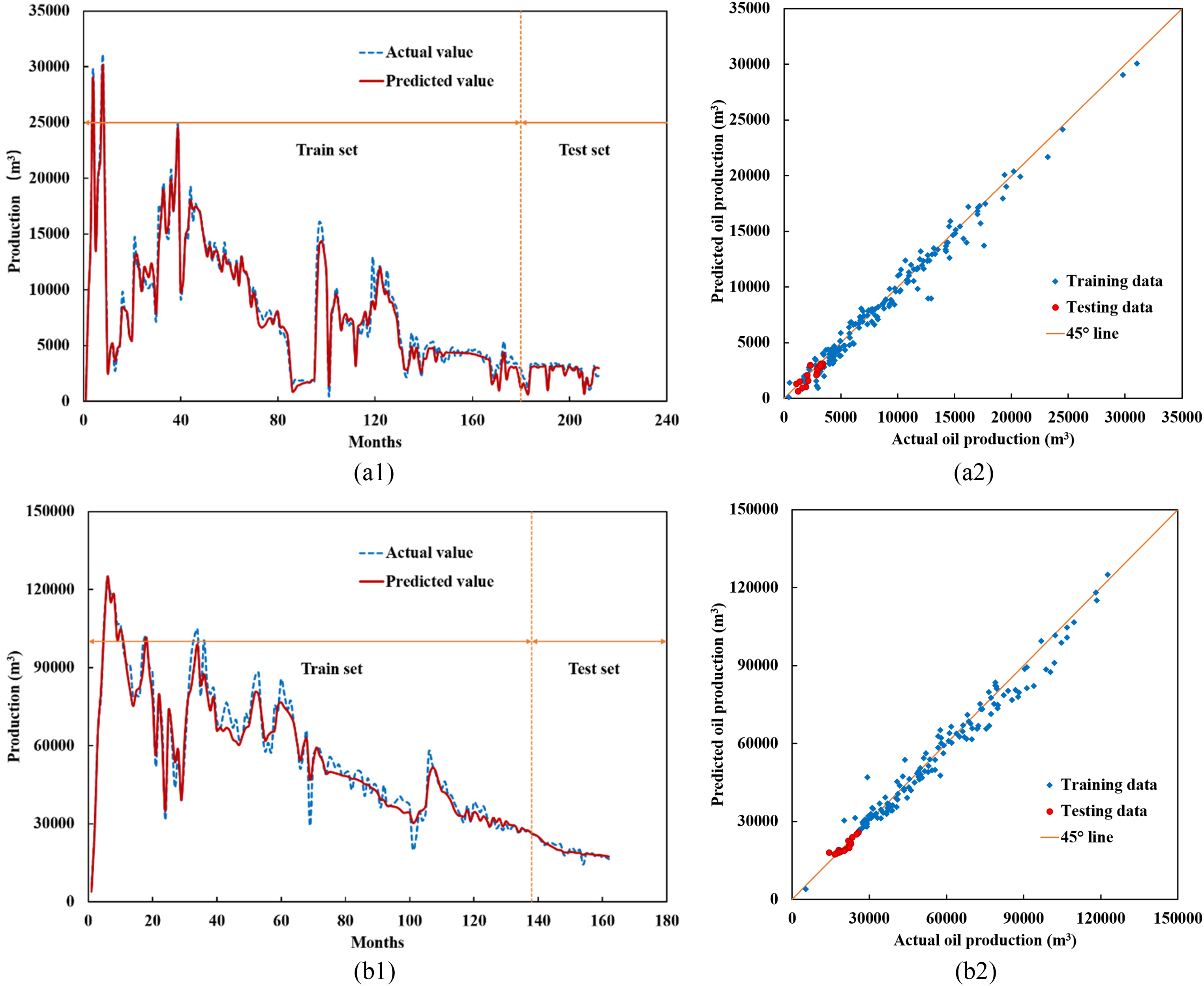
Comparison between actual production and predicted value of long short-term memory-based sequence-to-sequence model (Seq2Seq-LSTM): (a) Y-1 reservoir; (b) Y-2 reservoir.

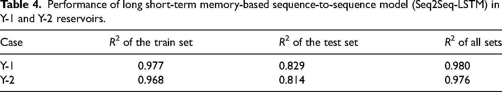
The predictive performance of Seq2Seq-LSTM is summarized in Table 4. When the coefficient of determination R² is close to 1, it indicates that the model is accurate. The R² of the test set in Y-1 and Y-2 reservoirs is 0.829 and 0.814, which means that the predictive performance of the proposed model is superior.

Table 4.

Performance of long short-term memory-based sequence-to-sequence model (Seq2Seq-LSTM) in Y-1 and Y-2 reservoirs.

Case	R² of the train set	R² of the test set	R² of all sets
Y-1	0.977	0.829	0.980
Y-2	0.968	0.814	0.976

In order to verify the superiority of the Seq2Seq-LSTM model, the traditional LSTM model is used to predict the oil production of the Y-1 reservoir. The oil production results predicted by the two methods from month 181 to month 212 are shown in Figure 9.

Figure 9.

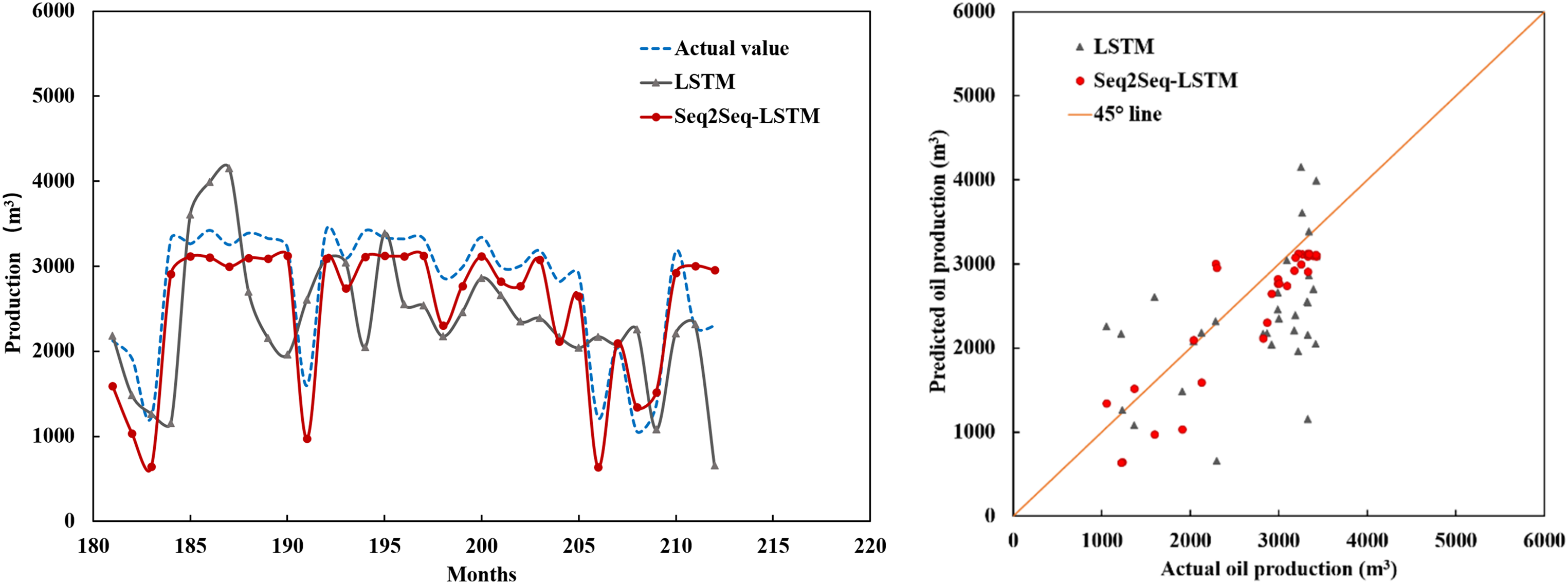
Comparison of prediction results of Seq2Seq-LSTM and LSTM in Y-1 reservoir.

According to the prediction results of the test set in the Y-1 reservoir, the R² of the LSTM model is 0.235, which is much lower than the 0.829 of the Seq2Seq-LSTM model, indicating that the prediction performance of Seq2Seq-LSTM model is significantly better than that of LSTM model. In the process of oil field production, liquid production and well spacing density are constantly adjusted, which has a great impact on oil production. The Seq2Seq-LSTM model can accurately predict the change in oil production after taking development measures because it learns the influence of liquid production and well spacing density change on oil production. However, the traditional LSTM model can only predict future oil production by relying on past oil production, so it can not reflect the impact of development measures on oil production.

In summary, the monthly oil production of reservoirs predicted by the method based on spatial–temporal data and Seq2Seq-LSTM is similar to the actual value. The advantage of the proposed model is that it can predict the oil production when liquid production and well spacing density of reservoirs change. Since the model learns the variation of oil production and features with time in multiple reservoirs through cross-learning, and explores the relationship between oil production and features, it can accurately predict the corresponding oil production even when liquid production and well spacing density are adjusted, which proves the reliability of the model.

Production prediction under different development measures

After verifying the reliability of the Seq2Seq-LSTM model driven by reservoir spatial-temporal data, taking the Y-2 reservoir as an example, the model is used to forecast the oil production in the next 24 months under different liquid production and well spacing density of reservoirs.

Figure 10 shows the predicted results of monthly oil production under different liquid production. The results show that if the current conditions remain unchanged, the trend of the predicted oil production is consistent with the declining trend of the original oil production. If the liquid production increased, the predicted oil production increased rapidly, then decreased rapidly and finally decreased slowly. If the increase of liquid production is larger, the predicted cumulative oil production is larger, which indicates that the oil production of the reservoir can be improved by increasing liquid production in this development stage. These reservoirs are developed using natural water energy without the need for additional water injection. Therefore, there is no need to consider the economic cost of increasing liquid production. In addition, the liquid production studied did not exceed the maximum liquid production in the history of the reservoir.

Figure 10.

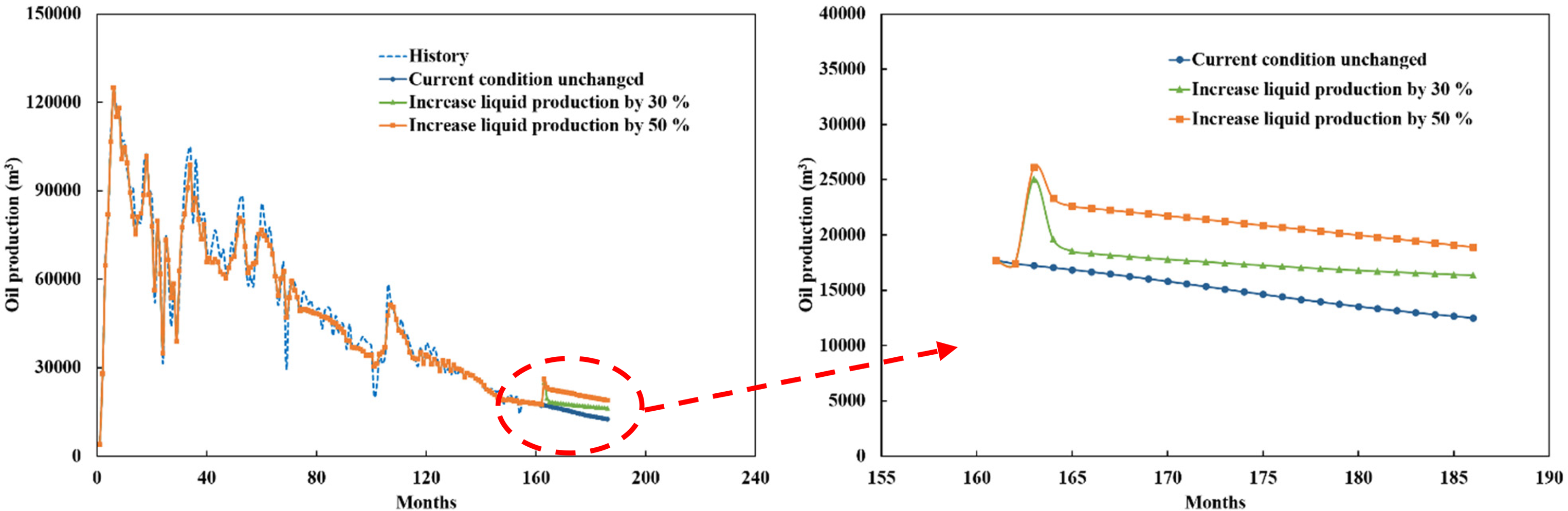
Predicted results of monthly oil production under different liquid production.

Figure 11 shows the predicted results of monthly oil production under different equivalent well spacing densities. The results show that if the equivalent well spacing density increased, the predicted oil production increased rapidly, then decreased slowly. If the number of equivalent vertical wells increases more, the predicted cumulative oil production is larger, which indicates that the oil production of the reservoir can be improved by increasing equivalent well spacing density in this development stage.

Figure 11.

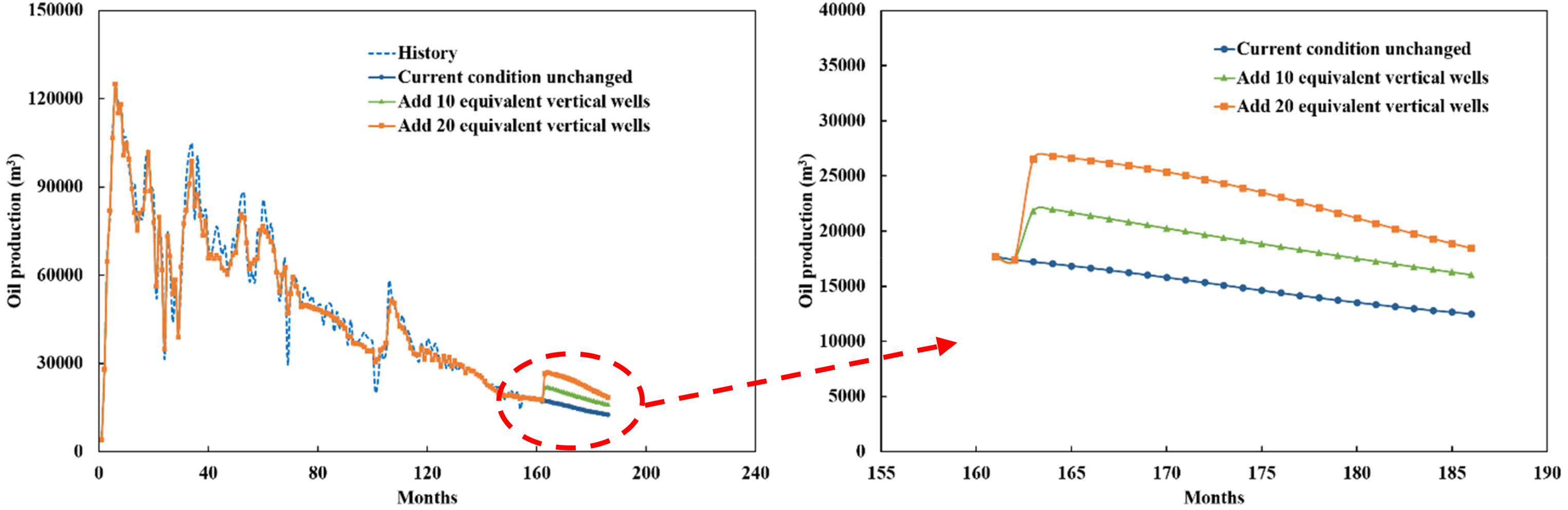
Predicted results of monthly oil production under different equivalent well spacing densities.

Since the Seq2Seq-LSTM model driven by reservoir spatial–temporal data learns the influence of changes in liquid production and well spacing density on oil production, it can accurately predict the oil production of the reservoir after taking development measures. Therefore, the method can be used as an effective way to predict oil production and analyse the remaining potential of reservoirs, which can help to adjust the reservoir development plan.

Conclusions

In this work, we took marine sandstone reservoirs in the Y basin as the research object to establish the sample database. Then, liquid production, production time, equivalent well spacing density, fluidity and original formation pressure were determined as input features according to the normalized mutual information. Finally, a Seq2Seq-LSTM model driven by reservoir spatial-temporal data was established to forecast oil production. By testing the performance of the proposed model on different samples, the following key conclusions are drawn:

A method of oil reservoir production prediction based on normalized mutual information and Seq2Seq-LSTM is proposed to forecast reservoir production considering the influence of liquid production and well spacing density. The Seq2Seq-LSTM model can not only learn the variation of production time series, but also learn the interaction from multiple samples and multiple sequences through cross-learning, and explores the relationship between oil production and every feature. It can be an alternative way for fast and accurate prediction of oil production considering the influence of liquid production and well spacing density in practical application.

Two case studies (Y-1 and Y-2 reservoirs) from the database are used to prove the proposed Seq2Seq-LSTM model. The coefficient of determination of the test set in Y-1 and Y-2 reservoirs are calculated to be 0.829 and 0.814, which means that the predictive performance of the proposed model is superior. Meanwhile, compared with the traditional LSTM model, the prediction performance of the proposed model is significantly better than that of the LSTM model.

Taking the Y-2 reservoir as an example, the proposed Seq2Seq-LSTM model is used to forecast the oil production in the next 24 months under different liquid production and well spacing density of reservoirs. The experimental results are in good agreement with the experience of the target oilfield. The method can be used as an effective way to predict oil production and analyse the remaining potential of reservoirs, which can help to adjust the reservoir development plan.

This study is equivalent to simplifying each reservoir. In order to forecast oil production more accurately, the factors affecting oil production can be considered more comprehensively in future work.

Footnotes

Declaration of conflicting interests

The author(s) declared no potential conflicts of interest with respect to the research, authorship, and/or publication of this article.

Funding

The author(s) disclosed the following financial support for the research, authorship, and publication of this article: This work received funding support from National Natural Science Foundation of China (51974343).

ORCID iD

Yin Qian

References

Arps

(1945) Analysis of decline curves. Transactions of the AIME 160(01): 228–247.

Bao

Gildin

Huang

, et al. (2020) Data-driven end-to-end production prediction of oil reservoirs by EnKF-enhanced recurrent neural networks. In: SPE Latin American and Caribbean petroleum engineering conference, Virtual, 27–31 July 2020.

Bhattacharya

Ghahfarokhi

Carr

, et al. (2019) Application of predictive data analytics to model daily hydrocarbon production using petrophysical, geomechanical, fiber-optic, completions, and surface data: a case study from the Marcellus shale, North America. Journal of Petroleum Science and Engineering 176: 702–715.

Castro

Souto

Ogasawara

, et al. (2021) STConvs2s: spatiotemporal convolutional sequence to sequence network for weather forecasting. Neurocomputing 426: 285–298.

Danon

Díaz-Guilera

Arenas

(2006) The effect of size heterogeneity on community identification in complex networks. Journal of Statistical Mechanics: Theory and Experiment 2006(11): 11010.

Dong

Zhang

Liu

, et al. (2021) Reservoir production prediction model based on a stacked LSTM network and transfer learning. ACS omega 6(50): 34700–34711.

Horng

(2018) Time series forecasting using sequence-to-sequence deep learning framework. In: International symposium on parallel architectures, algorithms and programming (PAAP), Taipei, Taiwan, China, 26–28 December 2018.

Wang

, et al. (2023) A systematic data-driven approach for production forecasting of coalbed methane incorporating deep learning and ensemble learning adapted to complex production patterns. Energy 263: 126121.

Fang

Crimier

Scanu

, et al. (2021) Multi-zone indoor temperature prediction with LSTM-based sequence to sequence model. Energy and Buildings 245: 111053.

10.

Gao

Liu

, et al. (2016) Coupled numerical simulation of multi-layer reservoir developed by lean-stratified water injection. Journal of Petroleum Exploration and Production Technology 6(4): 719–727.

11.

Guo

Zhao

You

, et al. (2021) Prediction of coalbed methane production based on deep learning. Energy 230: 120847.

12.

Hochreiter

Schmidhuber

(1997) Long short-term memory. Neural Computation 9(8): 1735–1780.

13.

Huang

Tian

Zhang

, et al. (2021) Support vector regression based on the particle swarm optimization algorithm for tight oil recovery prediction. ACS omega 6(47): 32142–32150.

14.

Ilk

Rushing

Perego

, et al. (2008) Exponential vs. hyperbolic decline in tight gas sands: understanding the origin and implications for reserve estimates using Arps’ Decline Curves. In: SPE annual technical conference and exhibition, Denver, CO, USA, 21–24 September 2008.

15.

Javier

Juan

JRA

José

AML

, et al. (2021) Artificial neural networks, sequence-to-sequence LSTMs, and exogenous variables as analytical tools for NO₂ (air pollution) forecasting: a case study in the bay of Algeciras (Spain). Sensors 21(5): 1770.

16.

Kingma

(2014) Adam: a method for stochastic optimization. arXiv:1412.6980.

17.

Liu

Yang

Liu

, et al. (2021a) Feature selection method based on mutual information and support vector machine. International Journal of Pattern Recognition and Artificial Intelligence 35(06): 2150021.

18.

Liu

Chen

Wang

, et al. (2017) A productivity prediction model for multiple fractured horizontal wells in shale gas reservoirs. Journal of Natural Gas Science and Engineering 42: 252–261.

19.

Liu

(2020) Forecasting oil production using ensemble empirical model decomposition based long short-term memory neural network. Journal of Petroleum Science and Engineering 189: 107013.

20.

Liu

Zhang

, et al. (2021b) A deep-learning-based prediction method of the estimated ultimate recovery (EUR) of shale gas wells. Petroleum Science 18(5): 1450–1464.

21.

Masoud

Mohammad

Osman

(2020) Data-driven hydrocarbon production forecasting using machine learning techniques. International Journal of Computer Science and Information Security 18: 65–72.

22.

Negash

Yaw

(2020) Artificial neural network based production forecasting for a hydrocarbon reservoir under water injection. Petroleum Exploration and Development 47(02): 383–392.

23.

Rodriguez

Salazar

(2022) Methodology for the prediction of fluid production in the waterflooding process based on multivariate long-short term memory neural networks. Journal of Petroleum Science and Engineering 208(PE): 109715.

24.

Sagheer

Kotb

(2018) Time series forecasting of petroleum production using deep LSTM recurrent networks. Neurocomputing 323: 203–213.

25.

Sang

Chen

Yang

, et al. (2014) A new mathematical model considering adsorption and desorption process for productivity prediction of volume fractured horizontal wells in shale gas reservoirs. Journal of Natural Gas Science & Engineering 19: 228–236.

26.

Song

Liu

Xue

, et al. (2020) Time-series well performance prediction based on long short-term memory (LSTM) neural network model. Journal of Petroleum Science and Engineering 186: 106682.

27.

Ullah

Zhang

Rehman

, et al. (2022) Linkages between trade openness, natural gas production and poverty in Pakistan: a simultaneous equation approach. Resources Policy 79: 103106.

28.

Valko

(2009) Assigning value to stimulation in the Barnett Shale: a simultaneous analysis of 7000 plus production histories and well completion records. In: SPE hydraulic fracturing technology conference, The Woodlands, TX, USA, 19–21 January 2009.

29.

Wang

Shi

, et al. (2020a) Production prediction at ultra-high water cut stage via recurrent neural network. Petroleum Exploration and Development 47(5): 1009–1015.

30.

Wang

Wan

, et al. (2020b) An analytical solution for transient productivity prediction of multi-fractured horizontal wells in tight gas reservoirs considering nonlinear porous flow mechanisms. Energies 13(5): 1066.

31.

Rui

Fan

, et al. (2020) Forecasting of coalbed methane daily production based on T-LSTM neural networks. Symmetry 12(5): 861.

32.

Xue

Liu

Xiong

, et al. (2021) A data-driven shale gas production forecasting method based on the multi-objective random forest regression. Journal of Petroleum Science and Engineering 196: 107801.

33.

Yang

Wang

(2020) A steam injection distribution optimization method for SAGD oil field using LSTM and dynamic programming. ISA Transactions 110: 198–212.

34.

Yang

Wang

, et al. (2021) Optimizing and accelerating history matching progress of numerical reservoir simulation by using material balance analysis. MATEC Web of Conferences 336(1): 01019.

35.

Zaytar

Amrani

(2016) Sequence to sequence weather forecasting with long short-term memory recurrent neural networks. International Journal of Computer Applications 143(11): 7–11.

36.

Zhang

Dou

Wang

, et al. (2022) A production prediction method of single well in water flooding oilfield based on integrated temporal convolutional network model. Petroleum Exploration and Development 49(5): 1150–1160.

37.

Zhang

Jia

(2021) Production performance forecasting method based on multivariate time series and vector autoregressive machine learning model for waterflooding reservoirs. Petroleum Exploration and Development 48(1): 175–184.

38.

Zhang

Wang

, et al. (2016) Research and application of hybrid PSO-BP neural network in fracture acidizing well production prediction. Revista de la Facultad de Ingeniería 31: 166–176.

39.

Zhang

Awotunde

(2016) Improvement of Levenberg-Marquardt algorithm during history fitting for reservoir simulation. Petroleum Exploration and Development 43(5): 876–885.

40.

Zhou

Wang

Zhu

(2021a) Feature selection based on mutual information with correlation coefficient. Applied Intelligence 52: 5457–5474.

41.

Zhou

Rao

, et al. (2021b) Artificial neural network- (ANN-) based proxy model for fast performances’ forecast and inverse schedule design of steam-flooding reservoirs. Mathematical Problems in Engineering 2021: 5527259.

Forecasting of oil production driven by reservoir spatial–temporal data based on normalized mutual information and Seq2Seq-LSTM

Abstract

Keywords

Introduction

Methodology

Modelling steps

Normalized mutual information

Long short-term memory

LSTM-based sequence-to-sequence model

Database establishment

Data pre-processing

Feature selection based on normalized mutual information

Modelling and application

Model training and structure optimizing

Result verification

Production prediction under different development measures

Conclusions

Footnotes

Declaration of conflicting interests

Funding

ORCID iD

References