
Abstract
We present a method that combines multiple sensory modalities in a rocket thrust chamber to predict impending thermoacoustic instabilities with uncertainties. This is accomplished by training an autoregressive Bayesian neural network model that forecasts the future amplitude of the dynamic pressure time series, using multiple sensor measurements (injector pressure/ temperature measurements, static chamber pressure, high-frequency dynamic pressure measurements, high-frequency OH* chemiluminescence measurements) and future flow rate control signals as input. The method is validated using experimental data from a representative cryogenic research thrust chamber. The Bayesian nature of our algorithms allows us to work with a dataset whose size is restricted by the expense of each experimental run, without making overconfident extrapolations. We find that the networks are able to accurately forecast the evolution of the pressure amplitude and anticipate instability events on unseen experimental runs 500 milliseconds in advance. We compare the predictive accuracy of multiple models using different combinations of sensor inputs. We find that the high-frequency dynamic pressure signal is particularly informative. We also use the technique of integrated gradients to interpret the influence of different sensor inputs on the model prediction. The negative log-likelihood of data points in the test dataset indicates that prediction uncertainties are well-characterized by our model and simulating a sensor failure event results in a dramatic increase in the epistemic component of the uncertainty, as would be expected when a Bayesian method encounters unfamiliar, out-of-distribution inputs.
Keywords
Introduction
High-frequency thermoacoustic instabilities are a potentially catastrophic phenomenon in rocket and aircraft engines. They usually arise from the coupling between unsteady heat release rate and acoustic eigenmodes of the combustion chamber. Acoustic waves incident on a flame cause fluctuations in its heat release rate. If a flame releases more (less) heat than average during instants of higher (lower) local pressure, then more work is done by the gas during the acoustic expansion phase than is done on it during the acoustic compression phase. If this work is not dissipated then the oscillation amplitude grows and the system becomes thermoacoustically unstable.
Thermoacoustic instabilities can be challenging to model and predict because they are usually sensitive to small changes in a combustion system. 1 The large pressure fluctuations and accelerated heat transfer caused by these oscillations can lead to structural failure, because rocket engines have high energy densities and low factors of safety in their structural design. From the F1 rocket engine, which underwent costly redesigns in the 1960s 2 to the modern Japanese LE-9 engine, 3 they continue to plague the development of liquid propellant rocket engines.
Designers can suppress thermoacoustic oscillations in two ways. The first method involves fitting passive devices such as acoustic liners, 2 baffles 4 and resonators 5 or the use of tuned passive control, where sensor measurements are used to diagnose thermoacoustic oscillations which can then be mitigated by adjusting a passive damping device or avoiding the operating point. 6 The second method is active feedback control. 7 The challenging demands of high power output, reliability and robustness placed on an active feedback control system means that feedback control is not used in rocket engines and aircraft engines. This paper proposes the diagnosis of impending instabilities using multiple sensor data-streams as input and Bayesian neural networks for forecasting. The forecast can be used by a rocket engine controller to perform a mass flow rate adjustment and avoid the unstable regions.
The remainder of the paper is paper is structured as follows. We provide an overview of related work in this field and explain the motivation behind the current study. Next, we describe the experimental rocket thrust chamber which generated our dataset. This is followed by details of the statistical tools we used: Bayesian neural network ensembles for forecasting and integrated gradients for interpreting them. We then compare the quality of the forecasts obtained using different model inputs and identify the influence of important input features on predictions using integrated gradients. We conclude with a brief summary of our findings and a discussion of potential avenues for future work.
The construction of instability precursors from pressure measurements and optical measurements has attracted considerable attention from the combustion research community, as reviewed by Juniper and Sujith. 8 Lieuwen 9 used the autocorrelation decay of combustion noise, filtered around an acoustic eigenfrequency, to obtain an effective damping coefficient for the corresponding instability mode. Other researchers have used tools from nonlinear time series analysis, which capture the transition from the chaotic behaviour displayed by stable turbulent combustors to the deterministic acoustics during instability, such as Gottwald’s 0-1 test 10 and the Wayland test for nonlinear determinism 11 to assess the stability margin of a combustor. Nair et al. 12 reported that instability is often presaged by intermittent bursts of high-amplitude oscillations and used recurrence quantification analysis (RQA) to detect these. In a later paper, Nair and Sujith 13 noted that combustion noise tends to lose its multifractality as the system transitions to instability. They proposed the Hurst exponent as an indicator of impending instability. Measures derived from symbolic time series analysis (STSA) 14 and complex networks 15 are also able to capture the onset of instability.
Recent studies have explored machine learning techniques to learn precursors of instability from data. These promise greater accuracy than physics-based precursors of instability, though at the cost of robustness and generalizability. Hidden Markov models constructed from the output of STSA 16 or directly from pressure measurements 17 have been used to classify the state of combustors. Hachijo et al. 18 have projected pressure time series onto the entropy-complexity plane and used support vector machines (SVMs) to predict thermoacoustic instability. SVMs were also employed by Kobayashi et al., 19 who used them in combination with principal component analysis and ordinal pattern transition networks to build precursors from simultaneous pressure and chemiluminiscence measurements. Sengupta et al. 20 showed that the power spectrum of the noise can be used to predict the linear stability of a thermoacoustic eigenmode using Bayesian neural networks. Related work by McCartney et al. 21 used the detrended fluctuation analysis (DFA) spectrum of the pressure signal as input to a random forest and found that this approach compared favorably to precursors from the literature. A recent study by Gangopadhyay et al. 22 trained a 3D Convolutional Selective Autoencoder on flame videos to detect instabilities. Nóvoa and Magri 23 adopt a hybrid approach, using Bayesian data assimilation to learn the parameters of a low fidelity model and an echo state network to model the forecast bias. Transfer learning is also being explored by Mondal et al. 24 as a means of efficiently transferring knowledge of precursors across machines.
Most papers in the literature identify indicators of approaching instability. In this study, on the other hand, we use nonlinear autoregressive time series modeling with a Bayesian Neural Network to forecast, with uncertainties, the future amplitude of pressure fluctuations given the history of sensor signals and future flow rate control signals. This informs the engine controller of the expected timing and potential severity of a forthcoming instability. This approach also lets us take advantage of the rich instrumentation of our rig by integrating multimodal sensor data into our model: high frequency dynamic pressure (
The size of our dataset is limited by the high cost and effort required for each additional test run on the rocket thrust chamber. Fortunately, the uncertainty-aware nature of the Bayesian Neural Network allows us to work in this medium-data regime without overconfident extrapolation. We compute log-likelihoods on the test dataset and find that the uncertainty is well-quantified. We also simulate a sensor failure to assess the robustness of our Bayesian forecasting tool. As expected, the network exhibits large epistemic uncertainties during the failure, signalling the unfamiliar out-of-distribution nature of the inputs. Finally we use the interpretation technique of integrated gradients (IG) to understand how the different input features in our model influence the predictions.
Experimental setup
The dataset used in this study is derived from experiments performed on the research combustor BKD
25
operated at the P8 test facility26,27 of the DLR Institute of Space Propulsion in Lampoldshausen. It has three main components: an injector head, a cylindrical combustion chamber and a convergent-divergent nozzle, as shown in Figure 1. The combustion chamber is water-cooled and is designed to deal with the high thermal loads that are expected during instability events. The L42 injector head has 42 shear coaxial injectors and is operated with a liquid oxygen (LOX)/ hydrogen (LH2) propellant combination. The cylindrical combustion chamber is 80 mm in diameter and the nozzle throat diameter is 50 mm, resulting in a contraction ratio of 2.56. The chamber static pressure (
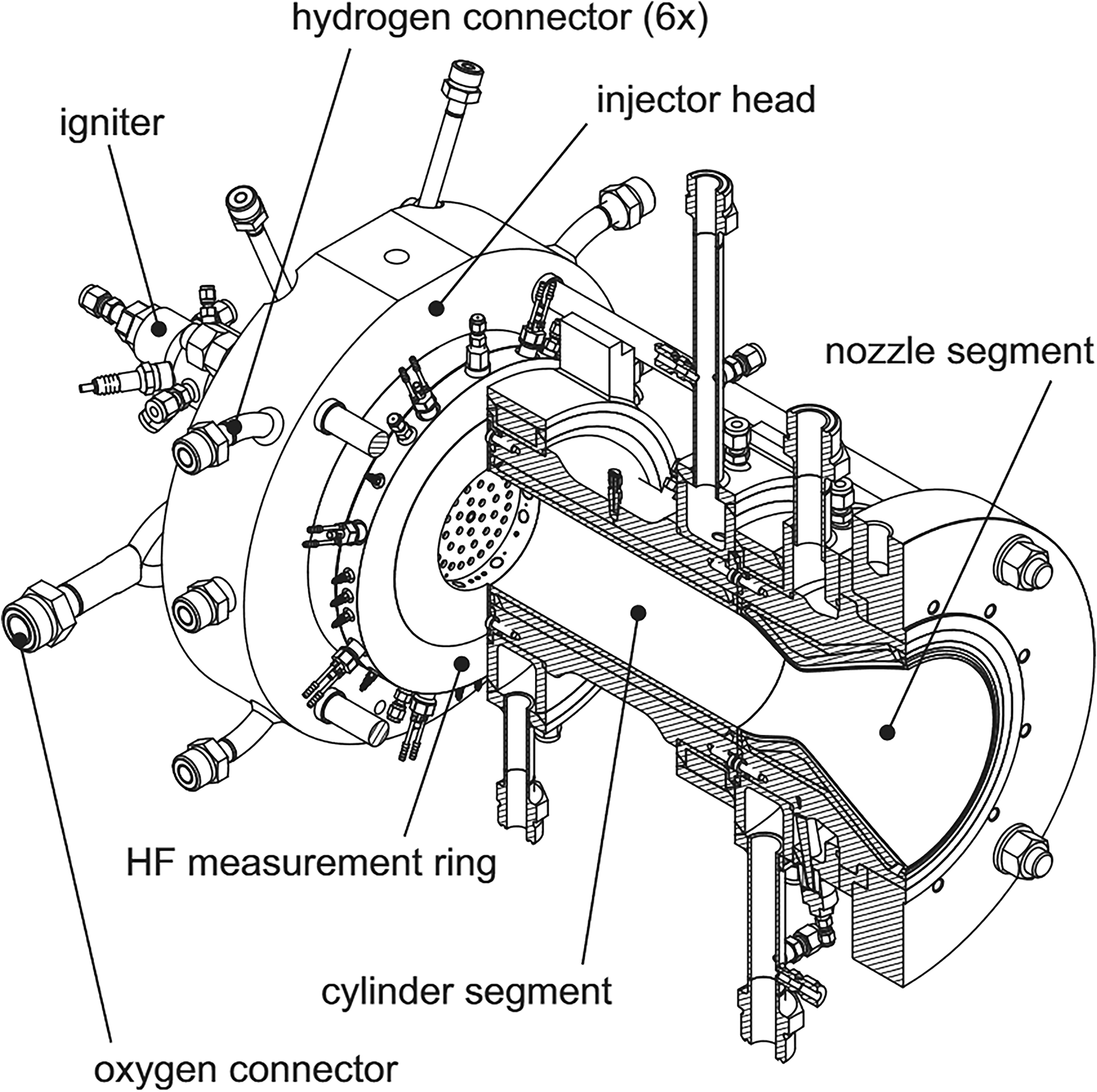
Experimental thrust chamber BKD.
For the operating point with
A representative BKD test sequence, along with a spectrogram of dynamic pressure oscillations inside the combustion chamber, is shown in Figure 2. Stable and unstable operating conditions can be identified in the spectrogram. Strong high-frequency combustion instabilities of the first tangential (1T) mode at about 10 kHz were excited consistently when approaching the operating point at
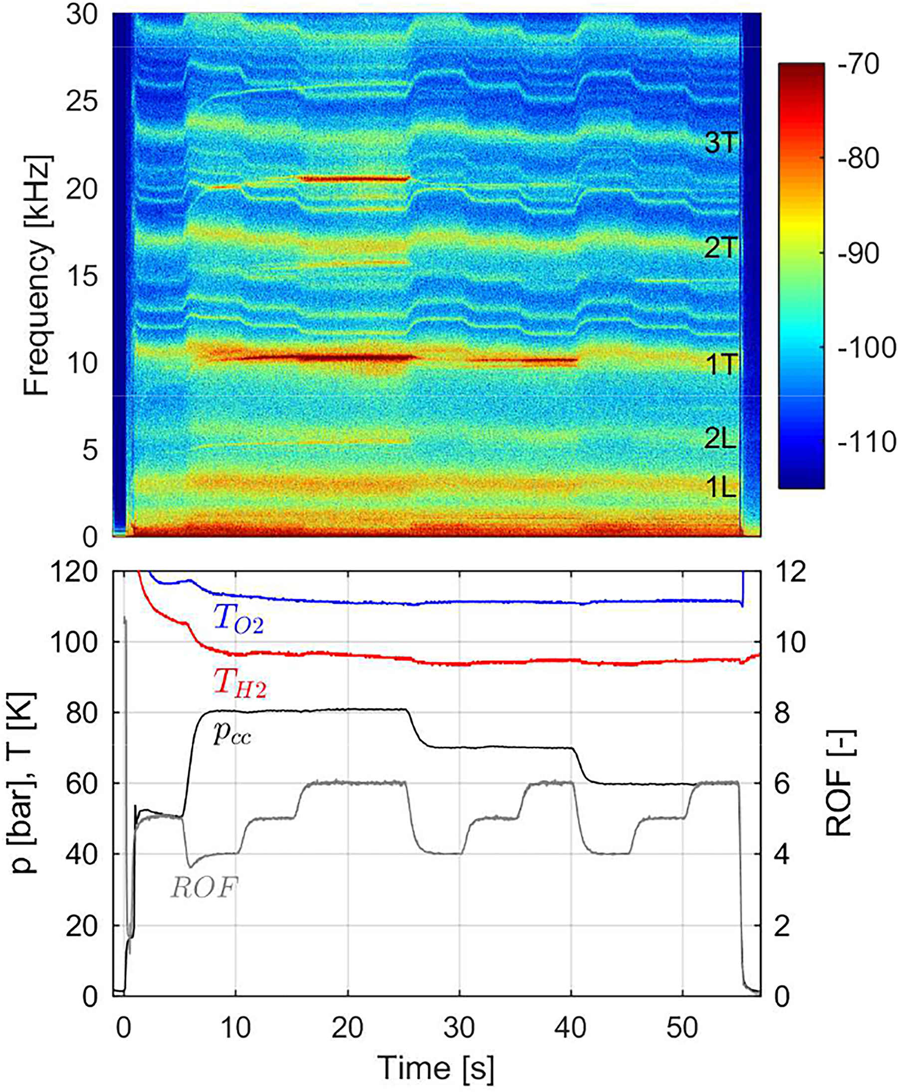
BKD test sequence and
The extreme conditions within the thrust chamber, where temperatures reach 3600 K and the pressure reaches 80 bar, limit the diagnostic instruments for our instability investigations. A specially designed measurement ring is placed between the injector head and the cylindrical combustion chamber segment, as shown in Figure 1. At this location, the temperatures are moderated by the injection of cryogenic propellants, which allows the mounted sensors to survive several test runs. Eight Kistler type 6043A water-cooled high-frequency piezoelectric pressure sensors are flush-mounted in the ring with an even circumferential distribution, in order to measure the chamber pressure oscillations
Methods
Nonlinear autoregressive models with exogenous variables (NARX) for timeseries modeling
To forecast instabilities, we train NARX-style models
29
to capture the functional relationship between the history of the sensor data, control signals and future pressure fluctuations. These model the evolution of pressure fluctuations as follows:
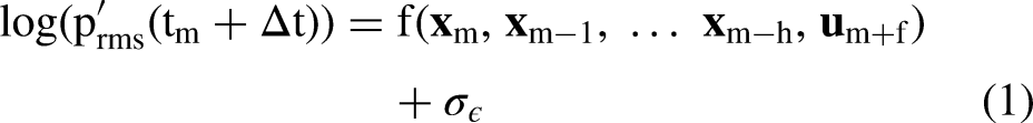
We model the nonlinear function
Bayesian neural network ensembles
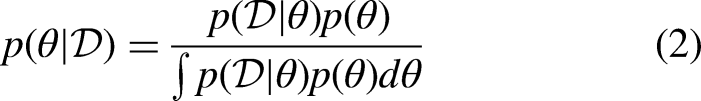
The Bayesian framework for training neural networks
30
involves placing a sensible prior probability distribution The parameters Each ensemble member is trained using a modified loss function that anchors the parameters to their initial values. The loss function for the
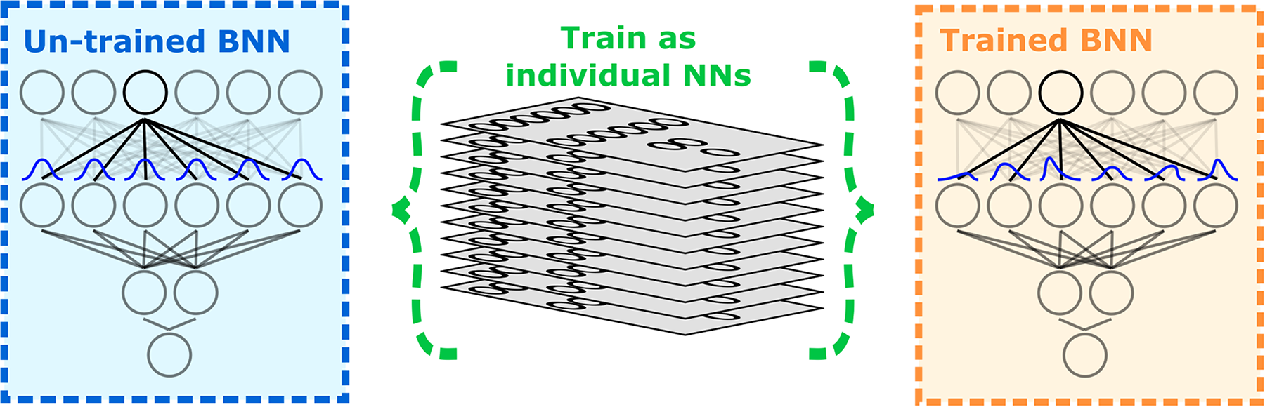
Approximate Bayesian inference using ensembles of neural networks.
Pearce et al.
33
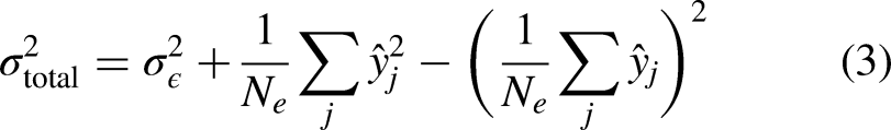
prove that this procedure approximates the true posterior distribution for wide neural networks and that the trained neural networks in the ensemble may be treated as samples from an approximate posterior distribution. The resulting ensemble has predictions that converge when they are well-supported by the training data and diverge when they are not. The variance of the ensemble predictions is an estimate of the Bayesian model’s epistemic uncertainty. Epistemic or knowledge uncertainty is the reducible portion of uncertainty which stems from uncertainty in model parameters and decreases as more data is added. The total uncertainty of each prediction is obtained by adding the epistemic uncertainty and the irreducible aleatoric uncertainty
Interpretation using integrated gradients
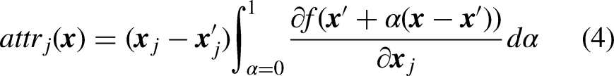
Neural networks have a reputation as black boxes, which disincentivizes their application to cases in which practitioners must understand why the algorithm is or is not working. We use the technique of integrated gradients (IG) 34 to attribute the predictions of our network ensemble to the input features. This is a simple scalable method that only requires access to the gradient operation. IG has several desirable properties that other attribution methods lack, such as implementation invariance, sensitivity, linearity, completeness and preservation of symmetry.
For deep neural networks, the gradients of the output with respect to the input are an analog of the linear regression coefficients. In a linear model, the regression coefficients characterize the relationship between input and output variables globally. In a nonlinear neural network, however, the gradient of the output at a point merely characterizes the local relationship between a predictor variable and the output. IG computes the path integral of the gradient of the outputs with respect to the inputs around a baseline to the input under consideration. For an image recognition algorithm, a completely black image could be a reasonable choice of baseline, while for a regression problem like ours, where the input variables were normalized to have zero mean and unit standard deviation, the average input of all zeros is a sensible baseline. We consider the straight-line path (in the feature space
Transforming sensor signals into neural network inputs
We compare NARX models with different combinations and transformations of the sensor data in their state variables
Models that include the low frequency signals
Kobayashi et al.
19
applied machine learning to the ordinal partition transition network of the
We also include a naive baseline model
Train-test-validation split, hyperparameters, performance metrics
We use a dataset of five experimental runs: three that are 50 seconds long and two that are 90 seconds long. Each run has two occurrences of the 1T instability, where an instability event is defined as being when the peak-to-peak amplitude of the pressure fluctuations exceeds 5% of the chamber static pressure.
To avoid data leakage, one experimental run is exclusively reserved for hyperparameter tuning. The timeseries is split into contiguous 250 millisecond blocks and every fifth block is used to evaluate the negative log-likelihood, which is the metric we use for tuning the BNN hyperparameters. The hyperparameters are the network depth, layer width, noise
To evaluate model performance, leave-one-out cross validation (LOOCV) is performed on the remaining four runs. Time series data involves strong temporal correlations, so assigning training and test data points randomly is dishonest because then the two sets would be highly similar. The test set must therefore be a completely independent experimental run. Additionally, LOOCV is necessary because with only four runs, firm conclusions cannot be drawn based on performance metrics for one particular test-train split, since any claimed efficacy or differences between models could be caused by chance. We report average performance metrics across the four possible splits.
To evaluate model accuracy, we compute the root mean squared error (RMSE) of our pressure amplitude forecast for the entire test run (full RMSE). We also calculate this on a subset of the test run comprising the two segments of the timeseries one second before and after a transition to instability event (transition RMSE). The RMSE is computed separately on this subset because our primary interest is in forecasting instabilities and the relative merits of different models become clearer on this subset where there is a dramatic change in the amplitude. As a measure of the quality of uncertainty, we report mean negative log-likelihood per test data point.
Results
The models were trained on a laptop with 16 GB RAM, an Intel i7-10870H CPU and an NVIDIA RTX 2070 GPU. Each NARX model took
Table 1 shows the average prediction RMSEs for the NARX models computed during cross-validation across the four runs. We note, firstly, that the NARX models outperform the naive baseline, which means that the data contains a predictable signal that can be extracted. We also observe that the simple models, which use only the two operating point parameters
Cross-validation RMSEs (in bar) for entire runs (Full RMSE) and the transition subset of the run (Transition RMSE) and mean negative log-likelihoods (NLL) for different NARX models. Lower RMSEs and NLLs are better.
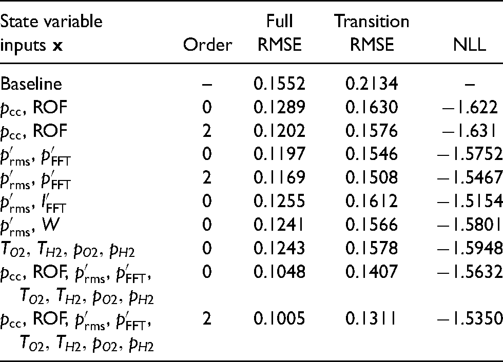
Table 1 also reports the mean negative log-likelihood (NLL) per datapoint, averaged across the four cross-validations. The mean negative log-likelihoods are fairly low for most of our models, implying that very few observations lie far outside the uncertainty bounds of the forecast (Figure 4). This is also confirmed by the percentage of data points in the test set within the
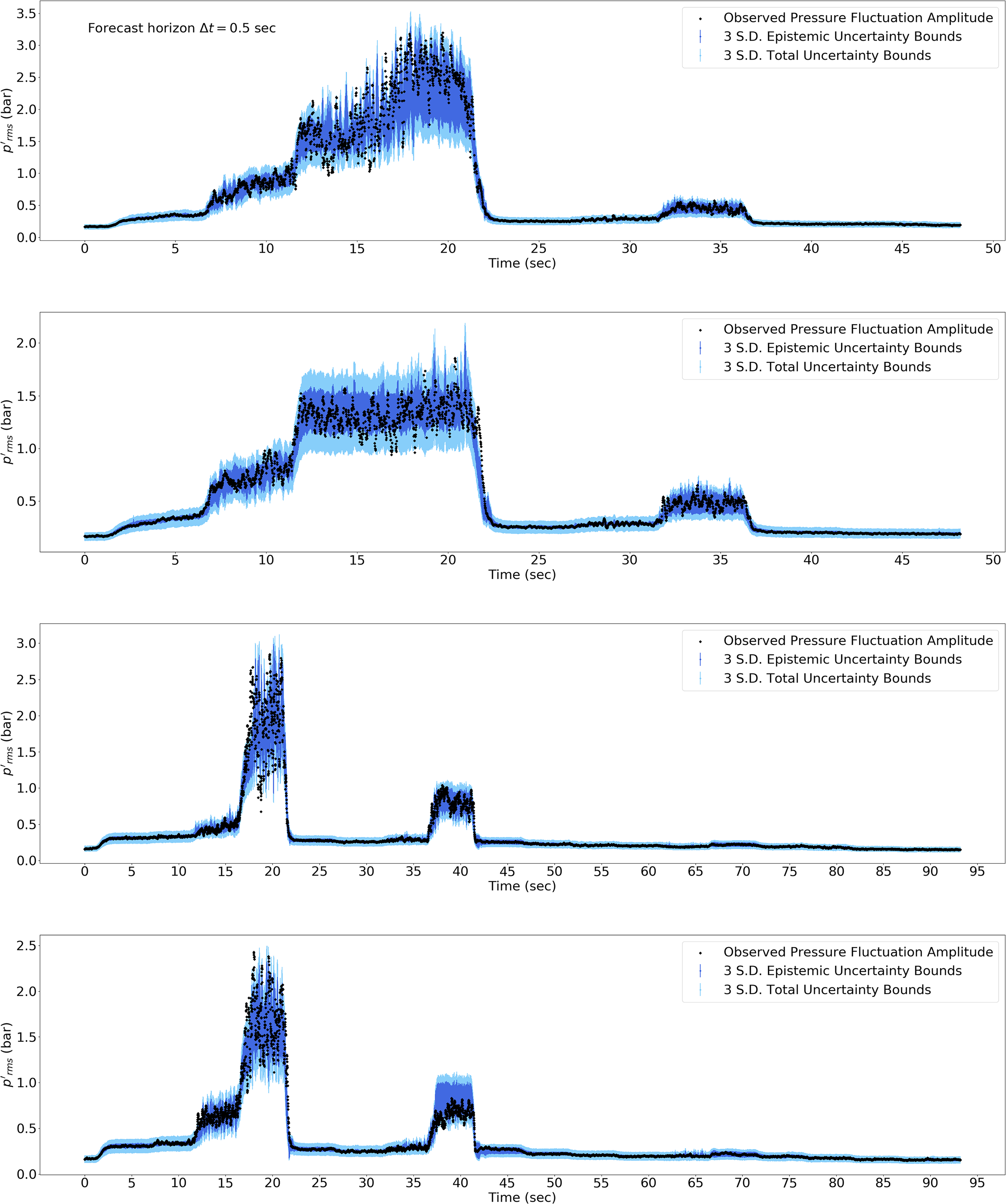
Forecast
To test the robustness of the Bayesian model against out-of-distribution inputs, we simulate a sensor failure event. This is shown in Figure 5. To simulate an optical probe icing event between 10 sec and 40 sec, the original photomultiplier signal is replaced by white noise with mean 0.05 and amplitude 0.015. During this simulated probe failure, the epistemic uncertainty of the Bayesian neural network greatly increases, indicating that the inputs are highly dissimilar to conditions experienced during training. Predictions remain reasonable despite the uninformative optical signal, although they become much less accurate.
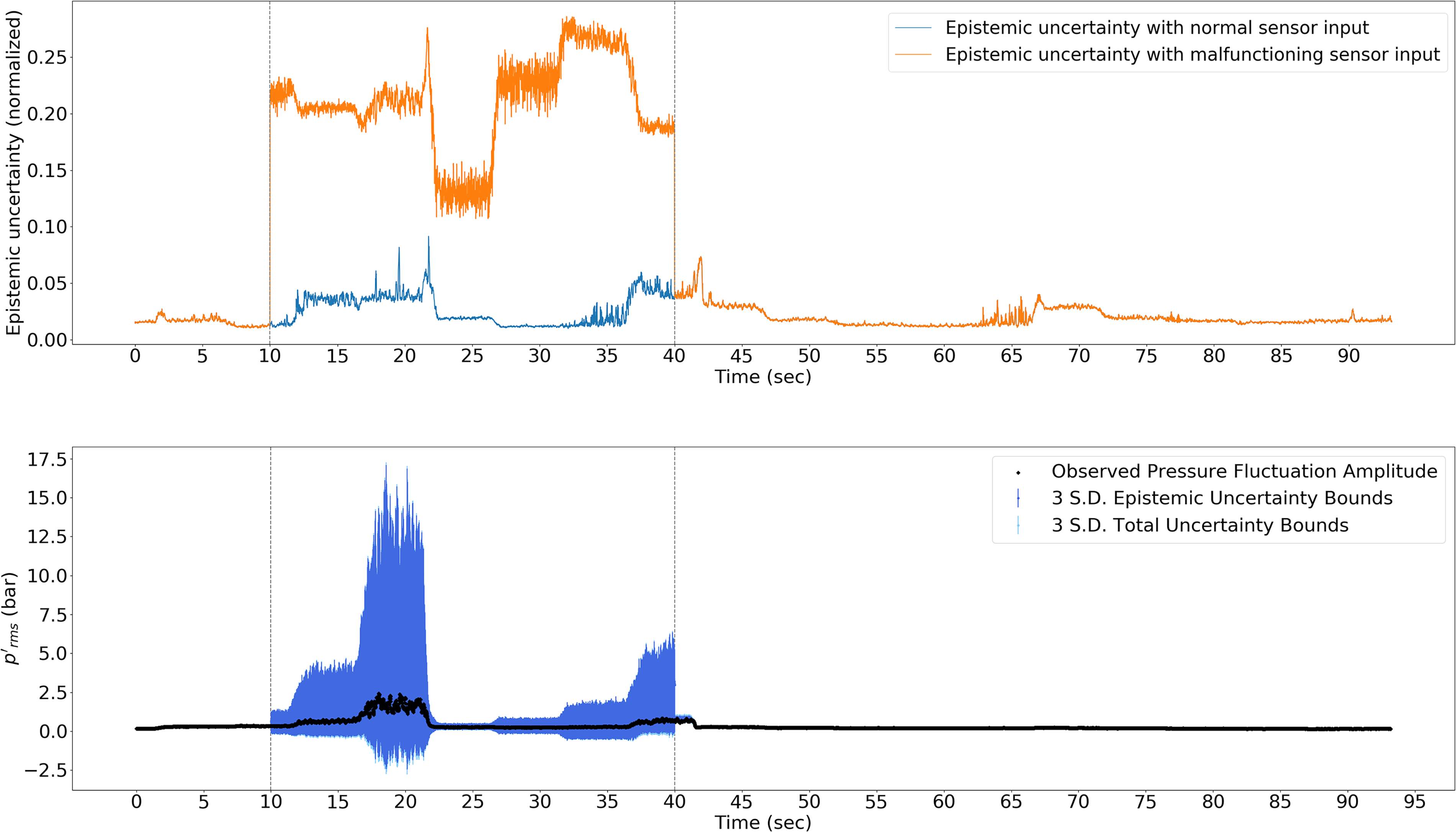
Bayesian Neural Network epistemic uncertainty (top) and
We use the technique of integrated gradients to produce feature-level attribution plots, which can tell us how much a particular predictor influenced the prediction for a particular input. For example, the attribution plots in Figure 6 shows this technique being applied to two data points. The first one is a data point just prior to the first instability event in a run, where a large jump in the dynamic pressure fluctuation amplitude is forecast by the model. This model uses
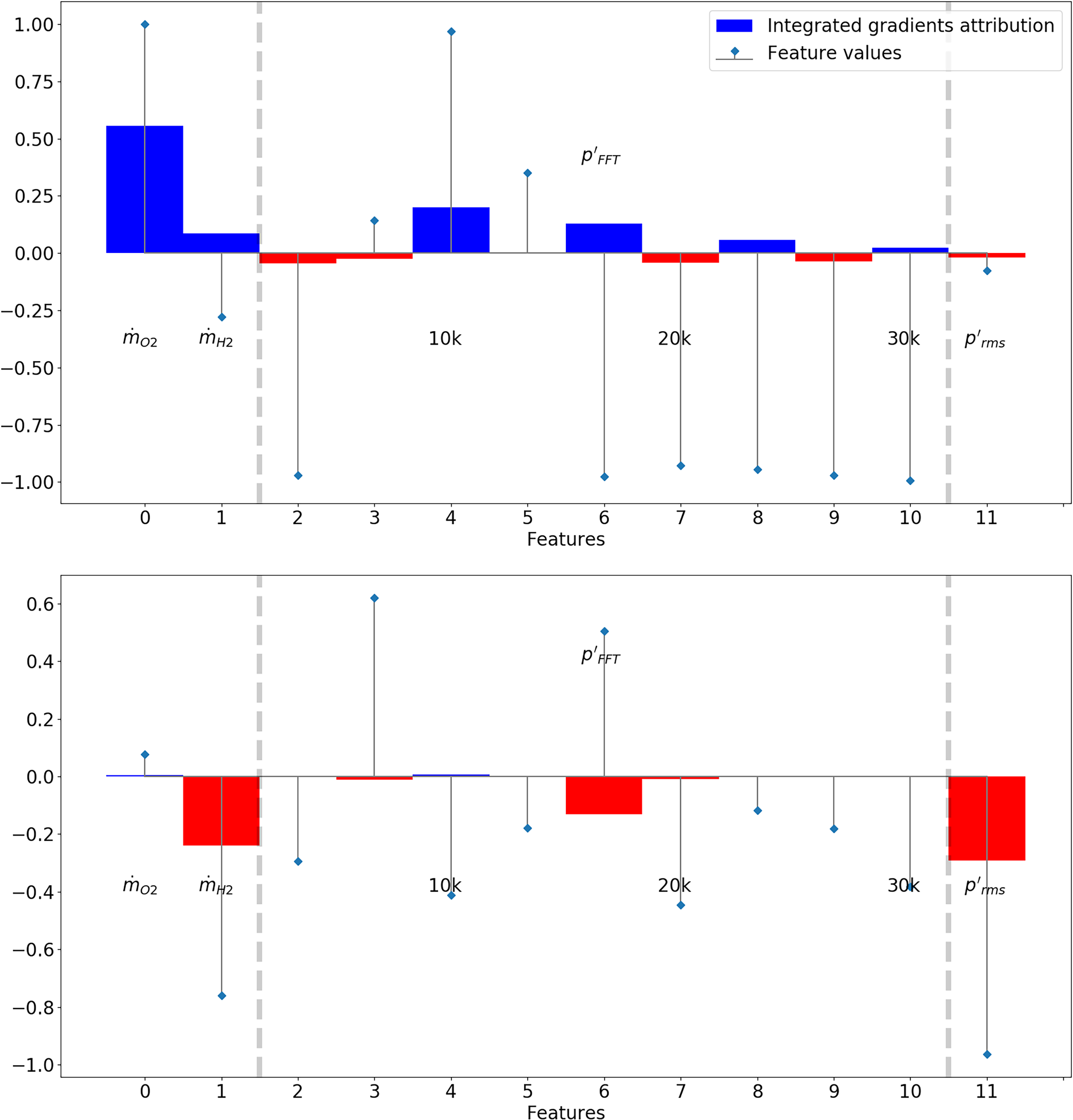
Integrated gradient attributions and input feature values (normalized to have zero mean and unit standard deviation) for two datapoints from experimental run no. 4 at t = 16.0 seconds (top, immediately preceding an instability) and t = 60.0 seconds (bottom, stable). The model used
Conclusions
In this paper, we present the application of an uncertainty-aware machine learning algorithm to forecast instabilities using multimodal sensor data in a realistic, thermoacoustically unstable rocket thrust chamber. We predict the amplitude of dynamic pressure fluctuations
A key benefit of our Bayesian approach is the ability to quantify the uncertainty in our predictions. In safety-critical machines such as rocket engines, a diagnostic tool must be robust to unexpected events such as sensor failures. We compute the log-likelihood of the test data given model predictions and find that uncertainties are well-characterized. We also simulate a sensor failure event in a model whose inputs included the spectrum of the fibre-optical probe signal and demonstrate the robustness of Bayesian algorithms. Integrated Gradients helps us identify important features and how they influence a particular prediction of the neural network.
Future work will focus on exploring the effectiveness of these tools on DLR’s other experimental datasets, such as the LOX-methane tests, which also displayed injection-coupled acoustic instabilities. 37 We will also explore the generalizability of data-driven diagnostics across multiple datasets and combustors, using approaches that utilise transfer learning or domain invariance. Hardware upgrades are currently being undertaken at the test facility that will allow the implementation of these methods into the engine control algorithm. 38
Footnotes
Acknowledgements
The authors would like to thank the crew of the P8 test bench and also Stefan Gröning for preparing and performing the test runs. Furthermore, we thank Wolfgang Armbruster for helping us process and understand the data. Ushnish Sengupta is an Early Stage Researcher within the MAGISTER consortium which receives funding from the European Union’s Horizon 2020 research and innovation programme under the Marie Skłodowska-Curie grant agreement No 766264.
Declaration of Conflicting Interests
The author(s) declared no potential conflicts of interest with respect to the research, authorship, and/or publication of this article.
Funding
The author(s) received no financial support for the research, authorship, and/or publication of this article.